A numerical model for the simulation of wave dynamics in the surf zone and near coastal structures
Bạn đang xem bản rút gọn của tài liệu. Xem và tải ngay bản đầy đủ của tài liệu tại đây (305.62 KB, 11 trang )
VNU Journal of Science, Earth Sciences 23 (2007) 160‐169
A numerical model for the simulation of wave dynamics
in the surf zone and near coastal structures
Vu Thanh Ca*
Center for Marine and Ocean-Atmosphere Interaction Research,
Vietnam Institute of Meteorology, Hydrology and Environment
Received 07 March 2007
Abstract. This paper describes a numerical model for the simulation of near shore wave dynamics
and bottom topography change. In this part, the nearshore wave dynamics is simulated by solving
the depth integrated Boussinesq approximation equations for nearshore wave transformation
together with continuity equation with a Crank‐Nicholson scheme. The wave runup on beaches is
simulated by a scheme, similar to the Volume Of Fluid (VOF) technique. The wave energy loss due
to wave breaking and shear generated turbulence is simulated by a k − ε model, in which the
turbulence kinetic energy (TKE) generation is assumed as the sum of those respectively due to
wave breaking and horizontal and vertical shear.
The verification of the numerical model against data obtained from various indoor experiments
reveals that the model is capable of simulating the wave dynamics, turbulence and bottom
topography change under wave actions. The simulation of turbulence in the surf zone and near
coastal structures enable the model realistically simulates the contribution of suspended sediment
transport into the bed topography change.
Keywords: Wave dynamics; Wave runup; Wave energy; Surf zone; Boussinessq model.
1. Introduction1
Nadaoka [9] found by indoor
experiments that during wave breaking, large
vortices were formed and rapidly extended
both vertically and horizontally. Ting and
Kirby [15‐17] by conducting experiments
with different wave conditions found that the
advective and diffusive transports of TKE
play a major role in the distribution of
turbulence, especially under plunging
breaker. They also found that under spilling
breakers (the breaking of relatively steep
waves on a gentle slope), the time variation of
TKE was relatively small, and the time
average transport of TKE was directed
offshore. Under plunging breakers (the
breaking of less steep waves on a gentle
slope), there was a large time variation of
Extensive researches on the wave
dynamics, sediment transport and bottom
topography change in the nearshore area,
especially in the surf zone [1‐5, 7, 9, 12, 14‐17]
have elucidated various aspects of coastal
processes, such as the dynamics of wave
breaking, characteristics of turbulence in the
surf zone, structure of the undertow, the
development of bottom boundary layer under
breaking waves, the rate of bed load transport,
uptake of bed material for suspension, settling
rate of suspended sediment etc.
_______
* Tel.: 84‐913212455.
E‐mail:
160
160
Vu Thanh Ca / VNU Journal of Science, Earth Sciences 23 (2007) 159‐168
TKE, and its time averaged transport is
directed on‐shore.
For situations with negligible alongshore
sediment transport, the status of a beach
depends on the cross‐shore transport of
sediment, which is closely related with wave
conditions. If the shoreward transport of
sediment by incoming waves exceeds the
offshore transport of sediment by retreating
waves and the undertow, there will be a net
onshore transport of sediment, resulting in
beach accretion. Otherwise, the beach is in
equilibrium state or eroded.
During a storm, turbulence generated by
the breaking of a relatively short wind wave
has not been significantly dissipated when a
new wave arrives and breaks. Thus, the time
variation of TKE is relatively small, and the
combination of wave‐induced flow and
undertow may transport TKE and suspended
sediment offshore. This results in the
offshore‐directed transport of sand during
storm and the associated beach erosion. On
the other hand, post storms, turbulence
generated by the breaking of a long period ‐
small amplitude swell has significantly
dissipated when the wave retreats. Thus,
there is a large time variation of TKE, and the
peaks in turbulence intensity and suspended
sediment concentration coincide with
incoming waves. Accordingly, onshore
transport of TKE and suspended sediment by
incoming waves exceeds the offshore
transport by retreating waves and the
undertow. This results in a net onshore
transport of suspended sediments and helps
explaining the onshore‐directed transport of
sediment during calm weather and the
consequent post storm beach recovery.
Schaffer [14] and Madsen [7] developed
models for the simulation of the nearshore
wave dynamics based on Boussinesq
approximation equations. The wave energy
loss due to breaking is simulated by
employing a surface roller model. Due to the
instability of the numerical code resulting
from the treatment of the surface roller wave
energy loss, Schaffer [14] had to use a
smoothing technique to stabilize the solution.
Rakha et al [12, 13] presented a quasi‐2D
and
a
quasi‐3D
phase
resolving
hydrodynamic and sediment transport
models. In these models, the horizontal
transport of TKE, and the associated
transport of suspended sediment are
neglected. However, as discussed previously,
results of Nadaoka et al [9] and Ting and
Kirby [16] show that the horizontal transport
of TKE in the surf zone is very important and
should not be neglected. Thus, without
accounting for this, it is not easy to simulate
the beach erosion during storm and the
consequent recovery after the storm.
Nadaoka and Ono [10] presented a depth‐
integrated k‐model where the TKE
production rate was evaluated with a
Rankine eddy model. In this model, the TKE
dissipation rate and the eddy viscosity was
evaluated by employing an empirical length
scale. The model had not been verified
against experimental data. Also, wave runup
on beach, which is mainly responsible for the
erosion of foreshore during storms, is not
simulated in this model.
Regarding all the above mentioned facts,
the purpose of this study is to develop a
numerical model that can simulate the
nearshore wave dynamics, including wave
breaking and wave runup, the generation,
transport and dissipation of TKE.
2. Governing equations of the numerical
model for nearshore wave dynamics
In this study, the near‐shore wave
Vu Thanh Ca / VNU Journal of Science, Earth Sciences 23 (2007) 159‐168
dynamics are simulated by solution of two‐
dimensional depth integrated Boussinesq
approximation equations, including bottom
friction and wave energy loss due to wave
breaking and shear. The main equations of
the numerical model are written as:
∂q x ∂q y ∂η
+
+
= 0
∂x
∂y
∂t
(1)
∂q x ∂ ⎛ q x2 ⎞ ∂ ⎛ q x q y ⎞
∂η
⎟ + gd
+ ⎜⎜ ⎟⎟ + ⎜⎜
∂t
∂x ⎝ d ⎠ ∂y ⎝ d ⎟⎠
∂x
h3 ⎡ ∂ 3 ⎛ qx ⎞
∂ 3 ⎛ q y ⎞⎤
⎜ ⎟⎥
+
(2)
⎢ 2 ⎜ ⎟+
6 ⎢⎣ ∂x ∂t ⎝ h ⎠ ∂x∂y∂t ⎜⎝ h ⎟⎠⎥⎦
∂ 3q y ⎞
h 2 ⎛ ∂ 3q
⎟ − M bx + f c Qq x = 0
− ⎜ 2x +
⎜
2 ⎝ ∂x ∂t ∂x∂y∂t ⎟⎠
d2
∂q y ∂ ⎛ q x q y ⎞ ∂ ⎛ q 2y ⎞
∂η
⎟ + ⎜ ⎟ + gd
+ ⎜⎜
∂t
∂x ⎝ d ⎟⎠ ∂y ⎜⎝ d ⎟⎠
∂y
h3 ⎡ ∂ 3 ⎛ q y ⎞
∂ 3 ⎛ q x ⎞⎤
⎜
⎟
(3)
+
+
⎜ ⎟⎥
⎢
6 ⎣⎢ ∂y 2 ∂t ⎜⎝ h ⎟⎠ ∂x∂y∂t ⎝ h ⎠⎦⎥
⎛ ∂ 3q y
∂ 3 q x ⎞⎟
f
⎜
+
− M by + c2 Qq y = 0
⎜ ∂y 2 ∂t ∂x∂y∂t ⎟
d
⎝
⎠
where q x and q y are respectively the depth
−
h2
2
integrated flow discharges in x and y
directions; η is the water surface elevation;
d is the instantaneous water depth; h is the
still water depth; f c is the bed friction
coefficient; Q is the total discharge, defined
as Q = q x2 + q 2y ; and M bx and M by represent
the wave energy loss due to breaking,
evaluated by introducing an eddy viscosity
and expressed as:
∂(q x / d ) ⎤ ∂ ⎡
∂(q x / d ) ⎤
∂ ⎡
+
df Dν t
df Dν t
∂x ⎢⎣
∂x ⎥⎦ ∂y ⎢⎣
∂y ⎥⎦
(4)
∂ qy / d ⎤ ∂ ⎡
∂ qy / d ⎤
∂ ⎡
=
⎢df Dν t
⎥+
⎢df Dν t
⎥
∂x ⎣
∂x ⎦ ∂y ⎣
∂y ⎦
M bx =
M by
(
)
(
)
In Eq. (4), ν t is the eddy viscosity; and f D
is an empirical coefficient, determined based
on the calibration of the numerical model.
161
When waves are breaking on beach, a
part of the lost wave energy is transformed
into turbulence energy. At the beginning of
the wave breaking process, the turbulence is
confined into a small portion of the breaking
wave crest, the surface roller; after that,
turbulence eddies rapidly expand in vertical
and horizontal directions [9, 15‐17]. The
turbulence under wave breaking is very
complex and fully three‐dimensional. Thus, a
3D model is required for a proper simulation
of turbulence processes here. However, such
a model would require an excessive
computational time and at the moment is not
suitable for a practical application. On the
other hand, based on results of Nadaoka et al
[9], Ting and Kirby [15‐17], it can be estimated
that in the surf zone, the time scale for
turbulence energy transport in the vertical
direction is much shorter than that in the
horizontal directions. Thus, the simulation of
the transport of TKE in the horizontal
direction is more important than that in the
vertical direction. Therefore, in the present
study, the TKE is assumed uniformly
distributed in the whole water depth, and the
depth‐integrated
equations
for
the
production, transport and dissipation of the
TKE and its dissipation rate read:
∂k ∂uk ∂vk
+
+
= Pr − ε
∂t
∂x
∂y
(5)
∂ ⎡ dν t ∂(k / d ) ⎤ ∂ ⎡ dν t ∂(k / d ) ⎤
+ ⎢
⎥+ ⎢
⎥,
∂x ⎣ σ t
∂x ⎦ ∂y ⎣ σ t
∂y ⎦
∂ε ∂uε ∂vε
∂ ⎡ dν ∂ (ε / d ) ⎤
+
+
= ⎢ t
⎥
∂t
∂x
∂y ∂x ⎣ σ ε
∂x ⎦
(6)
∂ ⎡ dν t ∂ (ε / d ) ⎤ ε
+ ⎢
⎥ + (C1ε Pr − C 2ε ε )
∂y ⎣ σ ε
∂y ⎦ k
where k and ε are respectively the depth
integrated TKE and its dissipation rate; u
and v are respectively phase‐depth
averaged flow velocities in x and y directions;
σ t , σ ε , C1ε , C2ε are closure coefficients. In
162
Vu Thanh Ca / VNU Journal of Science, Earth Sciences 23 (2007) 159‐168
Eq. (6), Pr is the TKE production rate, which
is assumed as a summation of the TKE
production due to bottom friction Prb ,
horizontal shear Prs and wave breaking Prw
as:
Pr = Prb + Prs + Prw
(7)
With known values of k and ε , the eddy
viscosity is evaluated as:
ν t = Cε k 2 / (dε ) ,
(8)
where Cε (= 0.09) is constant.
The scheme for the simulation of wave
runup and rundown on the beach is
explained in the next section. By employing
this scheme, the present model can simulate
the wave setup, set down on the beach, and
the erosion of foreshore during storm events.
3. Boundary and initial conditions and
numerical scheme
3.1. Boundary and initial conditions
It is possible to use a weekly wave
reflected boundary condition such as the
Summerfeld radiation condition at the
offshore boundary to let reflected waves
freely going out of the computational region.
However, this linear wave theory based
boundary condition, when applied in
combination with a nonlinear wave model,
does not ensure mass conservation and may
lead to an accumulation or lost of water
inside the computational region. Thus, in this
study, water surface elevation under waves is
given at the offshore boundary.
Wave‐absorbing zones are introduced at
the lateral boundaries to minimize wave
reflection. The bed friction coefficient f c in
these zones is assumed constant within first
five meshes from the lateral boundaries, and
then increases linearly with the distances
from the boundaries towards the ends of the
wave absorbing zones. Finally, at the ends of
the wave absorbing zones, the Summerfeld
radiation condition for long waves are
introduced to let remaining waves going out
of the computational region. A free slip
boundary condition is applied at surfaces of
the coastal structures.
Zero gradients of k and ε are assumed
at the offshore, lateral boundaries and at
surfaces of coastal structures.
A scheme similar to that of Hibberd and
Peregrine [5] is used to compute the wave
runup on the beach. A sketch of the scheme is
shown in Fig. 1. In this scheme, when the
shore is approached, all the dispersion terms
in Eqs. (2) and (3) are turned off.
Additionally, a cell side wetted function,
defined as the wetted portion over the total
length of a cell side, and a cell wetted area
function, defined as the wetted portion over
the total cell area are introduced to account
for the fact that water flows only in wetted
parts of the cells on the instantaneous
shoreline. Then, the continuity equation (Eq.
1) and momentum equations (Eqs. 2 and 3)
can be derived by a method similar to Vu et
al [19] and become:
∂f q
∂f q
∂Sη
y x + x y +
=0
(9)
∂x
∂y
∂t
∂q x 1 ∂ ⎛ Sq x2 ⎞ 1 ∂ ⎛ Sq x q y ⎞
⎜
⎟+
⎟
⎜
+
S ∂x ⎜⎝ d ⎟⎠ S ∂y ⎜⎝ d ⎟⎠
∂t
∂ (q x / d ) ⎤
∂η 1 ∂ ⎡
−
dν t S
∂x ⎥⎦
∂x S ∂x ⎢⎣
∂ (q x / d ) ⎤ f c
1 ∂ ⎡
dν t S
+
Qq x = 0,
−
S ∂y ⎢⎣
∂y ⎥⎦ d 2
+ gd
(10)
Vu Thanh Ca / VNU Journal of Science, Earth Sciences 23 (2007) 159‐168
2
⎞ 1 ∂ ⎛⎜ Sq y ⎞⎟
⎟⎟ +
∂t
⎠ S ∂y ⎜⎝ d ⎟⎠
∂ qy / d ⎤
∂η 1 ∂ ⎡
+ gd
−
⎢dν t S
⎥
∂y S ∂x ⎣
∂x ⎦
∂ qy / d ⎤ fc
1 ∂ ⎡
Qq y = 0
−
⎢ dν t S
⎥+
∂y ⎦ d 2
S ∂y ⎣
∂q y
+
1 ∂ ⎛ Sq y q x
⎜
S ∂x ⎜⎝ d
(
(
)
(11)
)
where f x and f y are respectively the cell side
wetted functions corresponding to x and y
directions, and S is the cell area wetted
function.
Fig. 1. The coordinate system and method for the
evaluation of a wetting and drying boundary.
The procedure for determining the cell
side wetted function and the cell area wetted
function in the numerical scheme will be
discussed in the next section.
A still water is assumed at the beginning
of the computation. With this, all variables
are set equal to zero initially.
3.2. Numerical scheme
Equations (1‐3) and (5‐6) are integrated
numerically on a spatially staggered grid
system, where components of the flow
discharge are evaluated at surfaces, and bed
elevation, k and ε are evaluated at the
centers of control volumes. The sketch of the
coordinates and computational mesh is
shown in Fig. 1. As it will be discussed later,
163
in the present scheme, the water level inside
a cell is evaluated at the center of the wetted
area inside the cell. A second order accurate
Crank‐Nicholson scheme is employed for the
time discretization for all equations, and a
central differencing scheme is employed for
spatial discretization of Eqs. (1) to (3). The
spatial disretization for advection terms of
Eqs. (5) and (6), governing the transport,
diffusion, generation and dissipation of k
and ε , follows the third order accurate
QUICK scheme, and that for the diffusion
terms follows the central differencing
scheme. As the discretization scheme is
implicit, an iterative scheme similar to the
SIMPLE scheme of Patankar [11] is
employed. At the beginning of a new time
step, the computation of the flow discharges
requires the still unknown water level and
eddy viscosity. Thus, at first, the water level
at each new time step is assumed equal to the
value at the previous time step. Then, Eqs. (2)
and (3) are solved to get the flow discharges
in x and y directions, respectively. The new
values of the flow discharges are substituted
into the continuity equation to compute the
new water level. Also, with the new water
level, the thickness of the surface roller is
evaluated. Then, Eqs. (5) and (6) are
integrated to get k and ε , and consequently
the new coefficient of eddy viscosity. All
newly obtained water level, flow discharges
and coefficient of eddy viscosity are
substituted back into Eqs. (2) and (3) to
compute the new components of the flow
discharge. The procedure is repeated until
converged solutions are reached.
The wetted periphery inside a
computational mesh at the intersection
between the water surface and the beach, the
cell side wetted function and the cell area
wetted function at each time step are
Vu Thanh Ca / VNU Journal of Science, Earth Sciences 23 (2007) 159‐168
164
evaluated explicitly based on the water level,
bed elevation and the bed slope in two
directions. The procedure for this is shown in
Fig. 1. The bed elevations at cell corners (such
as points A, B, C and D in Fig. 1) are evaluated
as the average value of the bed elevation at
four adjacent points. For example, the bed
elevation at point C in this figure is evaluated
as:
bc =
bi , j + bi , j +1 + bi +1, j +1 + bi +1, j
4
, (12)
where bc is the bed elevation at point C, and
bi,j, bi,j+1, bi+1,j+1 and bi+1,j are respectively the
bed elevations at the center of cells (i,j),
(i,j+1), (i+1,j+1) and (i+1,j).
The water level at a cell side is averaged
from the water levels at two adjacent cells.
For example, the water level on the side BC
of cell i,j in Fig. 1 is evaluated as:
ηbc =
ηi , j + ηi , j +1
2
,
(13)
where ηbc , ηi , j and ηi , j +1 are respectively
water levels at the cell side BC, and in the
cells (i,j) and (i,j+1).
If one of adjacent cells to a cell side is
completely dry (with the value of the area
wetted function equal to zero), the average
water level at the cell side is assumed equal
to the water level at the wetted cell. Based on
the bed elevation at its two ends and the
average water level on a cell side, the
intersected point between the water surface
and the cell side, and the wetted portion of
the side are determined. When the average
water level on the cell side is higher than the
bed elevation at its two ends, the side is
considered totally submerged into the water,
and the corresponding value of the cell side
wetted function is 1. For other cases, value of
the cell side wetted function equals to the
ratio of the length of the wetted portion over
the total length of the cell side. After getting
all the wetted points on four sides of the cell,
the wetted periphery and the wetted area
inside a cell are determined by connecting
two adjacent wetted points with a straight
line. This wetted periphery is shown by the
dotted line in Fig. 1. The wetted area in cell i,j
in this figure is the portion of the cell from
the dotted line to offshore. The wetted
periphery and area inside the cell are kept
constant for a time step.
4. Model verification
4.1. Wave transformation and characteristics of
turbulence due to wave breaking on a natural
beach
To verify the accuracy of the numerical
model on the simulation of the wave
transformation on a natural beach, existing
experimental data on the wave dynamics in
the nearshore area obtained by Ting and
Kirby [15‐17] are used. The experiments
were carried out in a two‐dimensional wave
flume of 40m long, 0.6m wide and 1.0m deep.
A plywood false bottom was installed in the
flume to create a uniform slope of 1 on 35.
Regular waves with heights and periods
equal to 12.7cm, 2s and 8.7cm, 5s are used as
incoming waves respectively for spilling
breaker and plunging breaker experiments.
Fig. 2 shows the sketch of the Ting and
Kirby [15‐17] experiments. Computation was
carried out with the same conditions of the
experiments. The critical water surface slope
for a broken wave to be recovered φ0 is set
equal to 60, according to Madsen et al [7].
Vu Thanh Ca / VNU Journal of Science, Earth Sciences 23 (2007) 159‐168
Wave generator
fD = a + b
1
0.38m
35
Fig. 2. Experiments by Ting and Kirby [15‐17].
As cited by various authors [2, 4], when
waves are breaking, a major part of the lost
wave energy is dissipated directly in the
shear layer beneath the surface roller, and only
a minor part of it is transformed into turbulent
energy. Thus, a turbulence model may
underestimate the wave energy lost due to
breaking. To account for this, an empirical
coefficient f D was introduced in Eq. 4.
Calibrations were carried out to find the best
value of this coefficient. Vu et al [18] found a
constant value of 1.5 for this coefficient for
their one‐dimensional model. However, their
computational results show that the
coefficient does not provide adequate wave
energy dissipation, and the computed wave
heights after breaking is significantly larger
than the observed ones.
As mentioned previously, wave breaking
happens with a sudden loss of wave energy.
This in a numerical model can be simulated
by a sudden increase in the “energy
dissipation coefficient” f D . As the breaking
wave progresses onshore, the growth of TKE
may accompany an increase in the coefficient.
On the other hand, turbulence length scale,
and the corresponding turbulence intensity
decrease with water depth, leading to a
decrease in the coefficient. Thus, in this
study, the coefficient is assumed suddenly
increases at the breaking point, then
gradually increases towards the shore, and
then decreases with the decrease in the water
depth in the following form:
2
⎛ hm ⎞
⎟
⎜
⎜ h ⎟ ,
⎝ mb ⎠
(14)
where a and b are constants, to be
determined from calibration; x and xb are
respectively the coordinates in the on‐
offshore direction at the point under
consideration and the breaking point; hm and
hmb are the corresponding mean water depths
at the respective points.
Fig. 3 shows the comparison between on‐
offshore distributions of time averaged mean
water surface elevation, minimum water
surface elevation, maximum water surface
elevation, and wave height for the spilling
breaker, computed by the model (with f D
evaluated following Eq. (14), a = 0.05 and
b = 1 ), and observed by Ting and Kirby [15,
16].
0.2
Height (m)
0.4m
x − xb
hmb
165
Bed
Comp. Etaav
Comp. Etamax
Comp. Etamin
Comp. Waveh
Obs. Wavh
Obs. Etaav
Obs. Etamax
Obs. Etamin
0.1
0
-0.1
-0.2
-0.3
-0.4
0 1 2 3 4 5 6 7 8 9 10 11 12 13
Horizontal Distance (m)
Fig. 3. Comparison between observed and computed
time averaged wave height, highest, lowest and
mean water surface elevation for spilling breaker.
Experimental data from Ting and Kirby [15, 16].
It can be seen in Fig. 3 that the model can
accurately predict the wave breaking point
and provides adequate wave energy
dissipation after breaking. The maximum,
minimum and mean water levels at all points
in the computational region are also
predicted by the model with good accuracy.
The general satisfactory agreement between
computed and observed data shown in the
Vu Thanh Ca / VNU Journal of Science, Earth Sciences 23 (2007) 159‐168
figure suggests that the model can simulate
nearshore wave processes, such as wave
energy loss due to breaking, wave setup,
setdown etc. with acceptable accuracy.
Figures (4) to (7) respectively show the
time variation of ensemble averaged (phase‐
averaged) non‐dimensional water surface
elevation, depth‐averaged horizontal flow
velocity, TKE, and advective transport rate of
TKE, computed by the model and observed
by Ting and Kirby [15, 16] at
(x − xb ) / hmb = 7.642 . The time t in the figures is
non‐dimensionalized by wave period T. For
convenient, the same coordinate system in
Ting and Kirby [15‐17] is employed in this
study. The computed time variation of
ensemble‐averaged water surface elevation
fluctuation, non‐dimensionalized by local
mean water depth hm (equal the sum of local
still water depth and mean water surface
fluctuation η ), shown in Fig. 4 agrees very
well with observed
between computed
variation of phase
horizontal
flow
dimensionalized by
data. The agreement
and observed time
and depth‐averaged
velocity,
non‐
the local long‐wave
commonly known that just after wave
breaking, turbulence is concentrated only
inside the surface roller, and flow in the
region below remains irrotational. Thus, a
depth‐integrated model for the generation,
transport and dissipation of TKE cannot be
considered as a good approximation for this
situation. However, despite of all inadequate
assumptions and approximations, order of
TKE predicted by the model, shown in Fig. 6,
agrees well with the observed one. Regarding
difficulties in predicting the TKE under wave
breaking with a numerical model, it can be
said that the numerical model can predict the
TKE and its advective transport with
satisfactory accuracy.
0.5
0.4
0.3
(ζ -<ζ >)/h
166
0.2
0.1
0
-0.1
-0.2
0
celerity c (defined as c = g (hm + H ) , with H
0.4
0.6
0.8
1
t/T
Fig. 4. Computed and observed phase‐averaged
water surface elevation at (x‐xb)/hb=7.462. Spilling
breaker.
0.4
0.3
0.2
<u >/c
as the deepwater wave height) also agrees
satisfactorily with observed data. The
agreement between computed and observed
phase and depth‐averaged non‐dimensional
TKE and its advective transport is less
satisfactory than that of the water level or
flow velocity. It must be noted that the
computation of TKE employs a depth‐
integrated k − ε model, which involves many
approximation assumptions and may not
accurately predict the TKE production,
transport and dissipation under a complex
situation such as wave breaking. Among all,
the weakest point of this model might be the
depth‐integrated approximation. It is
0.2
0.1
0
-0.1
-0.2
0
0.2
0.4
0.6
t /T
0.8
1
Vu Thanh Ca / VNU Journal of Science, Earth Sciences 23 (2007) 159‐168
2
Fig. 5. Computed and observed phase‐depth
averaged horizontal flow velocity
at (x-xb)/hb=7.462. Spilling breaker.
-
<u>k/c 3 (X10 3)
1.5
The agreement between computed and
observed advective transports of TKE, shown
in Fig. 7, is better than that for the TKE itself.
Results of Ting and Kirby [15, 16] show that
there is a tendency of offshore (negative)
transport of TKE. The computational results
by the present model also reveals the same
tendency; however, as shown in Fig. 8, the
residual advective offshore transport of TKE
evaluated by the numerical model is
significantly smaller than the observed one.
From the general agreement between
computed and observed values of various
wave characteristics, it can be remarked that
the numerical model can simulate wave
transformation in the nearshore region with
an acceptable accuracy.
0.006
0.005
k /c
2
0.004
0.003
0.002
0.001
0
0
0.2
0.4
0.6
0.8
1
t /T
Fig. 6. Computed and observed phase‐depth
averaged relative turbulent intensity
at (x-xb)/hb=7.462. Spilling breaker.
167
1.2
1
0.5
0
-0.5
-1
0
0.2
0.4
0.6
0.8
1
t /T
Fig. 7. Computed and observed phase‐depth
averaged relative advective transport rate of TKE
in the horizontal direction at (x-xb)/hb=7.462.
Spilling breaker.
4.2. Wave runup on beach
To verify the accuracy of the simulation
by the present numerical model on the wave
runup on beach, experimental data of Mase
and Kobayashi [8] are used. The sketch of the
experiment is shown in Fig. 10. As shown in
the figure, the experiments were carried out
in a wave flume with the length of 27 m,
depth of 0.75 m and width of 0.50 m. An
irregular wave generator is installed at one
end of the wave flume. At the other end is a
model beach with a foreshore slope of 1/20.
The water depth in front of the slope is set
constant and equal to 0.47 m. The wave runup
on the beach is recorded by a wave meter.
Wave groups used in the experiments are
expressed as:
η
1
1
= cos[2π (1 + δ ) ft ] + cos[2π (1 − δ ) ft ]
(15)
η max 2
2
= cos(2πδft )cos(2πft ),
where η max is the amplitude of the incoming
waves, f is the wave frequency, and ∆ is
the variation in the relative wave frequency.
During the experiments, η max was taken as 5
cm.
Vu Thanh Ca / VNU Journal of Science, Earth Sciences 23 (2007) 159‐168
168
Water Surface Elevation (m)
0.05
turbulence generated by wave breaking and
shear. As the model is a depth‐integrated,
two‐dimensional in the horizontal directions,
the computational time is relatively short.
Thus, the application of the model for
simulation of wave transformation in the
field, especially in the vicinity coastal
structures and inside harbours is very
promising.
0.025
0
- 0.025
- 0.05
0
5
10
15
Time (sec)
20
25
Fig. 8. Computed and observed wave runup height.
T = 2.5 s, ∆ = 0.1.
Fig. 8 shows an example of comparison
between observed and computed wave
runup for different wave periods. It can be
seen in the figures that the computed wave
runup heights agree very satisfactorily with
the observed values.
The computational results (not shown)
also reveal that short period waves are
dissipated much more rapidly on the beach
compared with long period waves. The very
satisfactory agreement between computed
and observed wave runup heights reveals
that the numerical model can accurately
simulate wave runup on beaches.
The model is also verified for its
applicability of computing waves near
coastal structures.
5. Conclusions
A numerical model has been developed
for the simulation of the wave dynamics in
the near shore area and in the vicinity of
coastal structures. It has been found that the
numerical model can satisfactorily simulate
the wave transformation, including wave
breaking, wave runup on the beach, and
References
[1] D. Cox, N. Kobayashi, Kinematic undertow
model with logarithmic boundary layer, Journal
of Waterway, Port, Coastal, and Ocean Engineering
123/6 (1997) 354.
[2] W.R. Dally, C.A. Brown, A modeling investigation
of the breaking wave roller with application to
cross‐shore currents, Journal of Geophysical
Research 100 (1995) 24873.
[3] A.G. Davies, J.S. Ribberink, A. Temperville, J.A.
Zyserman, Comparisons between sediment
transport models and observations made in
wave and current flows above plane beds,
Coastal Engineering 31 (1997) 163.
[4] R. Deigaard, Mathematical modelling of waves
in the surf zone, Prog. Report ISVA 69 (1989) 47.
[5] S. Hibberd, H.D. Peregrine, Surf and runup on
beach: A uniform bore, Journal of Fluid Mechanics
95 (1979) 323.
[6] C.W. Hirt, Nichols, Volume of fluid method for
the dynamics of free boundaries, Journal of
Computational Physics 39 (1981) 201.
[7] P.A. Madsen, O.R. Sorensen, H.A. Schaffer,
Surf zone dynamics simulated by a Boussinesq
type model. Part 1: Model description and cross‐
shore motion of regular waves, Coastal
Engineering 33 (1997) 255.
[8] H. Mase, N. Kobayashi, Low frequency swash
oscillation, Journal of Japan Society of Civil
Engineers II‐22/461 (1993) 49.
[9] K. Nadaoka, M. Hino, Y. Koyano, Structure of
the turbulent flow field under breaking waves
in the surf zone, Journal of Fluid Mechanics 204
(1989) 359.
Vu Thanh Ca / VNU Journal of Science, Earth Sciences 23 (2007) 159‐168
[10] K. Nadaoka, O. Ono, Time‐Dependent Depth‐
Integrated Turbulence Closure Modeling of
Breaking Waves, Coastal Engineering ACSE
(1998) 86.
[11] S.V. Patankar, Numerical Heat Transfer and Fluid
Flow, Hemisphere Publ. Co., London, 1980.
[12] K.A. Rakha, R. Deigaard, I. Broker, A phase
resolving cross shore sediment transport model
for beach profile evolution, Coastal Engineering
31 (1997) 231.
[13] K.A. Rakha, A quasi‐3D phase‐resolving
hydrodynamic and sediment transport model,
Coastal Engineering 34 (1998) 277.
[14] H.A. Schaffer, P.A. Madsen, R. Deigaard, A
Boussinesq model for waves breaking in
shallow water, Coastal Engineering 20 (1993) 185.
[15] F.C.K. Ting, J.T. Kirby, Observation of undertow
[16]
[17]
[18]
[19]
169
and turbulence in laboratory surf zone, Coastal
Engineering 24 (1994) 51.
F.C.K. Ting, J.T. Kirby, Dynamics of surf zone
turbulence in a strong plunging breaker, Coastal
Engineering 24 (1995) 177.
F.C.K. Ting, J.T. Kirby, Dynamics of surf zone
turbulence in a spilling breaker, Coastal
Engineering 27 (1996) 131.
Vu Thanh Ca, K. Tanimoto, Y. Yamamoto,
Numerical simulation of wave breaking by a k‐ε
model, Proceedings of Coastal Engineering, JSCE
47 (2000) 176.
Vu Thanh Ca, Y. Ashie, T. Asaeda, A k‐
ε turbulence closure model for the atmospheric
boundary layer including urban canopy,
Boundary‐Layer Meteorology 102 (2002) 459.