Tài liệu Hard Disk Drive Servo Systems- P4 ppt

136 5 Composite Nonlinear Feedback Control
can be expressed as for some non-negative variable .
Thus, for the case when
and , the closed-loop system
comprising the augmented plant in Equation 5.92 and the enhanced CNF control law
in Equation 5.101 can be expressed as follows:
(5.108)
In what follows, we show that the system in Equation 5.108 is stable provided
that the initial condition,
, the target reference, , and the disturbance, , satisfy
those conditions listed in the theorem. Let us define a Lyapunov function
(5.109)
For easy derivation, we introduce a matrix
such that . We then obtain the
derivative of
calculated along the trajectory of the system in Equation 5.108,
(5.110)
We note that we have used the following matrix properties: i)
,
where
is a symmetric matrix; ii) , if both and are square
matrices; and iii)
if and . Clearly, the closed-loop system
in the absence of the disturbance,
, has and thus is asymptotically stable.
With the presence of the unknown constant disturbance,
, and with the initial
condition
, where , the corresponding tra-
jectory of Equation 5.108 remains in
and converges to a point on a ball

with . Since converges to a constant,
it is clear that the tracking error
as . This completes the proof of
Theorem 5.8.
ii. Measurement Feedback Case. Next, we proceed to design an enhanced CNF
control law using only information measurable from the plant. In principle, we can
design either a full-order measurement feedback control law, for which its dynam-
ical order is identical to that of the given plant, or a reduced-order measurement
feedback control law, in which we make a full use of the measurement output and
estimate only the unknown part of the state variable. As such, the dynamical or-
der of the controller is reduced. It is more feasible to implement controllers with
smaller dynamical order. The procedure below on the enhanced CNF control using
Please purchase PDF Split-Merge on www.verypdf.com to remove this watermark.
5.2 Continuous-time Systems 137
reduced-order measurement feedback follows closely from that given in the previous
subsection.
For simplicity of presentation, we assume that
in the measurement output of
the given plant in Equation 5.89 is already in the form,
(5.111)
The augmented plant in Equation 5.92 can then be partitioned as follows:
sat
(5.112)
where
(5.113)
and
(5.114)
Clearly,
and are readily available and need not be estimated. We only need
to estimate

. There are two main step in designing a reduced-order measurement
feedback control laws: i) the construction of a full state feedback gain matrix
; and
ii) the construction of a reduced-order observer gain matrix
R
. The construction of
the gain matrix
is totally identical to that given in the previous subsection, which
can be partitioned in conformity with
, and , as follows:
(5.115)
The reduced-order observer gain matrix
R
is chosen such that the closed-loop poles
of
R
are placed in appropriate locations in the open-left half plane.
The reduced-order enhanced CNF control law is then given by,
R R
sat
R R R
(5.116)
and
R R
(5.117)
Please purchase PDF Split-Merge on www.verypdf.com to remove this watermark.
138 5 Composite Nonlinear Feedback Control
where is as defined in Equation 5.97 and is the smooth, nonpositive and
nondecreasing function of
, to be chosen to yield a desired performance.

Next, given a positive-definite matrix
, let be the
solution to the Lyapunov equation
(5.118)
Given another positive-definite matrix
R
with
R
(5.119)
let
R
be the solution to the Lyapunov equation
R R R R R
(5.120)
Note that such
and
R
exist as and
R
are both asymptotically
stable. We have the following result.
Theorem 5.9. Consider the given system in Equation 5.89 with
being bounded by
a scalar
, i.e. . Let
R
R R
R R R
(5.121)
Then, there exists a scalar

such that for any , a smooth and nonpositive
function of
with and tending to a constant as , the enhanced
reduced-order CNF control law of Equations 5.116 and 5.117 internally stabilizes
the given plant and drives the system controlled output
to track the step reference
of amplitude
asymptotically without steady-state error, provided that the following
conditions are satisfied:
1. There exist positive scalars
and
R
R
such that
R
R
R
(5.122)
2. The initial conditions,
and , satisfy
R
R
(5.123)
3. The level of the target reference,
, satisfies
(5.124)
where
is the same as that defined in Theorem 5.8.
Proof. The result follows from similar lines of reasoning as those in Theorem 5.8
and those for the measurement feedback case in the previous subsection.

Please purchase PDF Split-Merge on www.verypdf.com to remove this watermark.
5.2 Continuous-time Systems 139
5.2.3 Selection of Nonlinear Feedback Parameters
Basically, the freedom to choose the function
in either the usual CNF design or the
enhanced CNF design is used to tune the control laws so as to improve the perfor-
mance of the closed-loop system as the controlled output,
, approaches the set point,
. Since the main purpose of adding the nonlinear part to the CNF or the enhanced
CNF controllers is to shorten the settling time, or equivalently to contribute a sig-
nificant value to the control input when the tracking error,
, is small. The nonlinear
part, in general, is set in action when the control signal is far away from its saturation
level, and thus it does not cause the control input to hit its limits. For simplicity, we
now focus our attention on the case when the given system has external disturbances.
The following analysis is equally applicable to the case when the given system does
not have disturbances. Under such circumstances, the closed-loop system compris-
ing the augmented plant in Equation 5.92 and the enhanced CNF control law can be
expressed as:
(5.125)
We note that the additional term
does not affect the stability of the estimators. It
is now clear that eigenvalues of the closed-loop system in Equation 5.125 can be
changed by the function
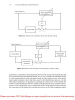
. Such a mechanism can be interpreted using the classical
feedback control concept as shown in Figure 5.1, where the auxiliary system
is defined as:
(5.126)
has the following interesting properties.
OUTPUT

Figure 5.1. Interpretation of the nonlinear function
Theorem 5.10. The auxiliary system defined in Equation 5.126 is stable
and invertible with a relative degree equal to
, and is of minimum phase with
stable invariant zeros.
Proof. First, it is obvious to see that is stable since is a stable
matrix. Next, since
and ,wehave
Please purchase PDF Split-Merge on www.verypdf.com to remove this watermark.
140 5 Composite Nonlinear Feedback Control
(5.127)
which implies that
is invertible and has a relative degree equal to (or an
infinite zero of order
). Furthermore, has invariant zeros, as it is a SISO
system.
The last property of
, i.e. the invariant zeros of are stable and
hence it is of minimum phase, can be shown by using the well-known classical root-
locus theory. Observing the block diagram in Figure 5.1, it follows from the classical
feedback control theory (see, e.g., [1]) that the poles of the closed-loop system of
Equation 5.125, which are the functions of the tuning parameter
, start from the
open-loop poles, i.e. the eigenvalues of
, when , and end up at the
open-loop zeros (including the zero at the infinity) as
. It then follows from
the proof of Theorem 5.3 that the closed-loop system remains asymptotically stable
for any nonpositive
, which implies that all the invariant zeros of the open-loop

system, i.e.
, must be stable.
It is clear from Theorem 5.10 and its proof that the invariant zeros of
play an important role in selecting the poles of the closed-loop system of Equation
5.125. The poles of the closed-loop system approach the locations of the invariant
zeros of
as becomes larger and larger. We would like to note that there
is freedom in preselecting the locations of these invariant zeros. This can actually
be done by selecting an appropriate
in Equation 5.98. In general, we should
select the invariant zeros of
, which are corresponding to the closed-loop
poles for larger
, such that the dominated ones have a large damping ratio, which
in turn yields a smaller overshoot. The following procedure can be used as a guideline
for the selection of such a
:
1. Given the pair
and the desired locations of the invariant zeros of
, we follow the result of Chen and Zheng [139] (see also Chapter 9 of
Chen et al. [71]) on finite and infinite zero assignment to obtain an appropri-
ate matrix
such that the resulting matrix triple has the
desired relative degree and invariant zeros.
2. Solve
for a . In general, the solution is nonunique
as there are
elements in available for selection. However, if the
solution does not exist, we go back to the previous step to reselect the invariant
zeros.

3. Calculate
using Equation 5.98 and check if is positive-definite. If is
not positive-definite, we go back to the previous step to choose another solution
of
or go to the first step to reselect the invariant zeros.
Generally, the above procedure would yield a desired result. The selection of the
nonlinear function
is relatively simple once the desired invariant zeros of
are obtained. Assuming the tracking error is available, the following choice of
is a smooth and nonpositive function of :
(5.128)
Please purchase PDF Split-Merge on www.verypdf.com to remove this watermark.
5.2 Continuous-time Systems 141
where and are appropriate positive scalars that can be chosen to yield a desired
performance, i.e. fast settling time and small overshoot. This function
changes
from
to as the tracking error approaches zero. At the
initial stage, when the controlled output,
, is far away from the final set point, is
small and the effect of the nonlinear part on the overall system is very limited. When
the controlled output,
, approaches the set point, , and the nonlinear
control law becomes effective. In general, the parameter
is chosen such that the
poles of
are in the desired locations, e.g., the dominated poles
have a large damping ratio, which would reduce the overshoot of the output response.
Note that the choice of
is nonunique. Any function would work so long as it has

similar properties of that given in Equation 5.128.
5.2.4 An Illustrative Example
We illustrate the enhanced CNF control technique for continuous-time systems in the
following example. We consider a continuous-time system of Equation 5.89 with
(5.129)
(5.130)
and
. The disturbance is unknown. For simulation purpose, we assume
. Our goal is to design an enhanced CNF state feedback control law that
would yield a good transient performance in tracking a target reference
.
Following the procedure given in the previous subsection, we select an integra-
tion gain
and obtain an appropriate augmented system. After a few tries, we
found that the following state feedback gain to the augmented system would yield a
good performance for our problem:
(5.131)
which places the poles of
at , , . We note that the
first one corresponds to the integrator. Both the linear state feedback control and
enhanced CNF control share the same integration dynamics:
(5.132)
The linear state feedback control law is given by
(5.133)
Letting
diag , we obtain a positive-definite solution for
Equation 5.98, which is given by
(5.134)
Please purchase PDF Split-Merge on www.verypdf.com to remove this watermark.
142 5 Composite Nonlinear Feedback Control

and an enhanced CNF state feedback law:
(5.135)
where
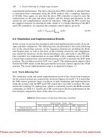
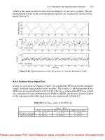
is as given in (5.128) with and . The simulation results given
in Figures 5.2 and 5.3 clearly show that the CNF control has outperformed the linear
control.
0
2
4
6
8
10
12
14
16
18
20
0
0.2
0.4
0.6
0.8
1
1.2
1.4
Time (s)
Output response
Linear control
Enhanced CNF control
Figure 5.2. Output responses of the enhanced CNF control and linear control

5.3 Discrete-time Systems
As in the continuous-time case, we present in this section the CNF design technique
for systems without and with external disturbances. Selection and interpretation of
nonlinear gain design parameters are also discussed.
5.3.1 Systems without External Disturbances
Let us now consider a linear discrete-time system
with an amplitude-constrained
actuator characterized by
Please purchase PDF Split-Merge on www.verypdf.com to remove this watermark.
5.3 Discrete-time Systems 143
0
2
4
6
8
10
12
14
16
18
20
0.4
0.6
0.8
1
1.2
1.4
1.6
1.8
2

Time (s)
Control signals
Linear control
Enhanced CNF control
Figure 5.3. Control signals of the enhanced CNF control and linear control
sat
(5.136)
where
, , and are, respectively, the state, control input,
measurement output and controlled output of
. , , and are appropriate
dimensional constant matrices, and sat:
represents the actuator saturation
defined as
sat
sgn (5.137)
with
being the saturation level of the input. The following assumptions on the
system matrices are required:
1.
is stabilizable,
2.
is detectable, and
3.
is invertible and has no invariant zeros at .
We now extend the results of the continuous-time composite nonlinear control
method to the discrete-time system in Equation 5.136. Thus, the objective here is
to design a discrete-time CNF control law that causes the output to track a high-
amplitude step input rapidly without experiencing large overshoot and without the
adverse actuator saturation effects. This can be done through the design of a discrete-

time linear feedback law with a small closed-loop damping ratio and a nonlinear
feedback law through an appropriate Lyapunov function to cause the closed-loop
Please purchase PDF Split-Merge on www.verypdf.com to remove this watermark.
144 5 Composite Nonlinear Feedback Control
system to be highly damped as system output approaches the command input to re-
duce the overshoot. The result of this discrete-time version is analogous to that of
its continuous-time counterpart. Here, we again separate the design of discrete-time
CNF control into three distinct situations, i.e. 1) the state feedback case, 2) the full-
order measurement case, and 3) the reduced-order measurement feedback case.
i. State Feedback Case. We consider the case when
, i.e. all the state variables
of
of Equation 5.136 are available for feedback.
S
TEP
5.
D
.
S
.1: design a linear feedback law,
L
(5.138)
where
is the input command, and is chosen such that has all its
eigenvalues in
and the closed-loop system meets
certain design specifications. We note again that such an
can be designed
using any of the techniques reported in Chapter 3. Furthermore,
(5.139)

We note that
is well defined because has all its eigenvalues in ,
and
is invertible and has no invariant zeros at .
The following lemma determines the magnitude of
that can be tracked by such
a control law without exceeding the control limits.
Lemma 5.11. Given a positive-definite matrix
, let be the solution
of the following Lyapunov equation:
(5.140)
Such a
exists as is asymptotically stable. For any , let
be the largest positive scalar such that
(5.141)
Also, let
(5.142)
and
(5.143)
Then, the control law in Equation 5.138 is capable of driving the system controlled
output
to track asymptotically a step command input of amplitude , provided
that the initial state
and satisfy:
and (5.144)
Please purchase PDF Split-Merge on www.verypdf.com to remove this watermark.
5.3 Discrete-time Systems 145
Proof. Let . Then, the linear feedback control law
L
can be rewritten as

L
(5.145)
Hence, for all
(5.146)
and for any
satisfying
(5.147)
the linear control law can be written as
L
(5.148)
which indicates that the control signal
L
never exceeds the saturation. Next, let
us move to verify the asymptotic stability of the closed-loop system comprising the
given plant in Equation 5.136 and the linear feedback law in Equation 5.138, which
can be expressed as follows:
(5.149)
Let us define a Lyapunov function for the closed-loop system in Equation 5.149 as
(5.150)
Along the trajectories of the closed-loop system in Equation 5.149 the increment of
the Lyapunov function in Equation 5.150 is given by
(5.151)
This shows that
is an invariant set of the the closed-loop system in Equation
5.149 and all trajectories of Equation 5.149 starting from
converge to the origin.
Thus, for any initial state
and the step command input that satisfy Equation
5.144, we have
(5.152)

and hence
(5.153)
This completes the proof of Lemma 5.11.
Remark 5.12. We would like to note that, for the case when , any step com-
mand of amplitude
can be tracked asymptotically provided that
and (5.154)
This input command amplitude can be increased by increasing
and/or decreasing
through the choice of . However, the change in affects the damping
ratio of the closed-loop system and hence its rise time.
Please purchase PDF Split-Merge on www.verypdf.com to remove this watermark.
146 5 Composite Nonlinear Feedback Control
S
TEP
5.
D
.
S
.2: the nonlinear feedback control law
N
is given by
N
(5.155)
where
is a nonpositive scalar function, locally Lipschitz in , and is to be
used to change the system closed-loop damping ratio as the output approaches
the step command input. The choice of
will be discussed later in detail.
S

TEP
5.
D
.
S
.3: the linear and nonlinear components derived above are now com-
bined to form a discrete-time CNF control law:
L N
(5.156)
We have the following result.
Theorem 5.13. Consider the discrete-time system in Equation 5.136. Then, for any
nonpositive
, locally Lipschitz in and , the
CNF control law in Equation 5.156 is capable of stabilizing the given plant and
driving the system controlled output
to track the step command input of am-
plitude
from an initial state , provided that and satisfy the properties in
Equation 5.144.
Proof. Let . Then, the closed-loop system can be written as
(5.157)
where
sat
N
(5.158)
Equation 5.144 implies that
Define a Lyapunov function
(5.159)
Noting that
(5.160)

we can evaluate the increment of
along the trajectories of the closed-loop sys-
tem in Equation 5.157 as follows:
(5.161)
Next, we proceed to find the increment of
for three different cases, as is done
in continuous-time systems.
If
N
then
Please purchase PDF Split-Merge on www.verypdf.com to remove this watermark.
5.3 Discrete-time Systems 147
N
(5.162)
Thus,
(5.163)
For any nonpositive
with , it is clear that the increment
If
N
then implies that
N
and Hence,
N
N N
N
(5.164)
Thus, for all
,wehave , and hence
(5.165)

Similarly, for the case when
N
it can be shown
that
.
Thus,
is an invariant set of the closed-loop system in Equation 5.157 and
all trajectories of Equation 5.157 starting from
remain there and converge to the
origin. This, in turn, indicates that, for all initial states
and the step command
input of amplitude
that satisfy Equation 5.144,
(5.166)
and
(5.167)
This completes the proof of Theorem 5.13.
Remark 5.14. Theorem 5.13 shows that the addition of the nonlinear feedback con-
trol law
N
as given in Equation 5.155 does not affect the ability to track the class of
command inputs. Any command input that can be tracked by the linear feedback law
in Equation 5.138 can also be tracked by the CNF control law in Equation 5.156. The
composite feedback law in Equation 5.156 does not reduce the level of the trackable
command input for any choice of the function
. This freedom can be used to
improve the performance of the overall system. The choice of
will be dis-
cussed in the forthcoming subsection.
ii. Full-order Measurement Feedback Case. We proceed to construct a discrete-

time full-order CNF control law in the following.
Please purchase PDF Split-Merge on www.verypdf.com to remove this watermark.
148 5 Composite Nonlinear Feedback Control
S
TEP
5.
D
.
F
.1: we first construct a linear full-order measurement feedback control
law
sat
L
L
(5.168)
where
is the command input, is the state of the controller, and
are chosen such that and have all their eigenvalues in , i.e.
both are stable matrices, and, furthermore, the resulting closed-loop system has
met certain design specifications. As usual, we let
(5.169)
and
(5.170)
We note that both
and are well defined.
Lemma 5.15. Given a positive-definite matrix
P
, let be the solution
to the Lyapunov equation
P

(5.171)
Given another positive-definite matrix
Q
with
Q
P
(5.172)
let
be the solution to the Lyapunov equation
Q
(5.173)
Note that such
and exist as and are asymptotically stable.
For any
, let be the largest positive scalar such that for all
F
(5.174)
we have
(5.175)
The linear control law in Equation 5.168 drives the system controlled output
to
track asymptotically a step command input of amplitude
from an initial state ,
provided that
, and satisfy:
and
F
(5.176)
Please purchase PDF Split-Merge on www.verypdf.com to remove this watermark.
5.3 Discrete-time Systems 149

Proof. This follows along similar lines to the reasoning given in the proofs of Lem-
mas 5.5 and 5.11.
S
TEP
5.
D
.
F
.2: the discrete-time full-order measurement composite nonlinear feed-
back control law is given by
sat (5.177)
and
(5.178)
where
is a nonpositive scalar function, locally Lipschitz in , and is to be
chosen to improve the performance of the closed-loop system.
We have the following result.
Theorem 5.16. Consider the given discrete-time system in Equation 5.136. Then,
there exists a scalar
such that for any nonpositive function
, locally Lipschitz in and , the discrete-time CNF control law in
Equations 5.177 and 5.178 internally stabilizes the given plant and drive the system
controlled output
to track asymptotically the step command input of amplitude
from an initial state , provided that , and satisfy the conditions in Equation
5.176.
Proof. The proof of this theorem follows along similar lines to the reasoning given
in Theorems 5.6 and 5.13.
iii. Reduced-order Measurement Feedback Case. As in its continuous-time coun-
terpart, we now proceed to design a reduced-order measurement feedback controller.

For the given system in Equation 5.136, it is clear that
states of the system are mea-
surable if
is of maximal rank. As such, we could design a dynamic controller that
has a dynamical order less than that of the given plant. We now proceed to construct
such a control law under the CNF control framework.
For simplicity of presentation, we assume that
is already in the form
(5.179)
Then, the system in Equation 5.136 can be rewritten as
sat
(5.180)
and
Please purchase PDF Split-Merge on www.verypdf.com to remove this watermark.
150 5 Composite Nonlinear Feedback Control
(5.181)
where the original state
is partitioned into two parts, and with .
Thus, we only need to estimate
in the reduced-order measurement feedback de-
sign. Next, we let
be chosen such that 1) is asymptotically stable, and
2)
has the desired properties, and let
R
be chosen such
that
R
is asymptotically stable. Again, it follows from Chen [110] that
is detectable if and only if is detectable. Thus, there exists a sta-

bilizing
R
. Again, such and
R
can be designed using any of the linear control
techniques presented in Chapter 3. We then partition
in conformity with and
:
(5.182)
As defined in Equations 5.169 and 5.169, we let
(5.183)
and
(5.184)
The reduced-order CNF controller is given by
R R
sat
R R R
(5.185)
and
R
R
(5.186)
where
is a nonpositive scalar function locally Lipschitz in subject to certain
constraints to be discussed later.
Next, given a positive-definite matrix
P
, let be the solution to
the Lyapunov equation
P

(5.187)
Given another positive-definite matrix
R
with
R
P
(5.188)
let
R
be the solution to the Lyapunov equation
R R R R R
(5.189)
Please purchase PDF Split-Merge on www.verypdf.com to remove this watermark.
5.3 Discrete-time Systems 151
Note that such and
R
exist as and
R
are asymptotically
stable. For any
, let be the largest positive scalar such that for all
R
R
(5.190)
we have
(5.191)
We have the following theorem.
Theorem 5.17. Consider the system given in Equation 5.1. Then, there exists a
scalar
such that for any nonpositive function , lo-

cally Lipschitz in
and , the reduced-order CNF control law given by
Equations 5.185 and 5.186 internally stabilizes the given plant and drives the system
controlled output
to track asymptotically the step command input of amplitude
from an initial state , provided that , and satisfy
R
R
and (5.192)
Proof. Again, the proof of this theorem is similar to those given earlier.
5.3.2 Systems with External Disturbances
We consider a linear discrete-time system with actuator saturation and disturbances
characterized by
sat
(5.193)
where
, , , and are, respectively, the state, control
input, measurement output, controlled output and disturbance input of the system.
,
, , and are appropriate dimensional constant matrices. The function, sat:
, represents the actuator saturation defined as
sat
sgn (5.194)
with
being the input saturation level. The following assumptions on the given
system are made:
1.
is stabilizable,
2.
is detectable,

3.
is invertible with no invariant zero at ,
4.
is bounded unknown constant disturbance, and
Please purchase PDF Split-Merge on www.verypdf.com to remove this watermark.
152 5 Composite Nonlinear Feedback Control
5. is part of , i.e. is also measurable.
We aim to design a discrete enhanced CNF control law for the system with input
saturation and disturbances to track a step reference, say
, neither violating the input
saturation nor having steady-state bias. An equivalent discrete integration, which
eventually becomes part of the final control law, is defined as follows,
(5.195)
where the tracking error
is available for feedback as is assumed
to be measurable and
is a positive scalar to be selected to yield an appropriate
integration speed. By integrating Equation 5.195 into the given system, we obtain
the following augmented system
sat
(5.196)
where
(5.197)
(5.198)
and
(5.199)
We note that under Assumptions 1 and 3, it is straightforward to verify that the pair
is stabilizable.
In what follows, we proceed to design an enhanced CNF control laws for the
given system for two different cases, i.e. the state feedback case and the reduced-

order measurement feedback case. The full-order measurement feedback case can
be solved in a straightforward manner once the result for the reduced-order case is
established.
i. State Feedback Case. We consider in the following the situation when all the
state variables of the given system in Equation 5.193 are measurable, i.e.
. The
procedure that generates an enhanced CNF state feedback law is done in three steps.
That is, in the first step, a linear feedback control law with appropriate properties is
designed, then in the second step, the design of nonlinear feedback portion is carried
out, and lastly, in the final step, the linear and nonlinear feedback laws are combined
to form an enhanced CNF control law.
S
TEP
5.
D
.
W
.
S
.1: Design a linear feedback control law,
L
(5.200)
Please purchase PDF Split-Merge on www.verypdf.com to remove this watermark.
5.3 Discrete-time Systems 153
where is chosen such that i) is asymptotically stable, and ii) the
closed-loop system
has certain desired properties. Let us
partition
in conformity with and . The general guide-
line in designing such a state feedback gain

is to place the closed-loop pole
of
corresponding to to be sufficiently closer to compared
to the other eigenvalues, which implies that
is a relatively small scalar. The
remaining closed-loop poles of
are placed to have a dominating pair
with a small damping ratio, which in turn would yield a fast rise time in the
closed-loop system response. Finally,
is chosen as
(5.201)
which is well defined as
is assumed to have no invariant zeros at
and is nonsingular whenever is stable and is
relatively small.
S
TEP
5.
D
.
W
.
S
.2: Given an appropriate positive-definite matrix ,
we solve the following Lyapunov equation:
(5.202)
for
. Such a solution is always existent as is asymptotically stable.
The nonlinear feedback portion of the enhanced CNF control law,
N

, is then
given by
N
(5.203)
where
, with , is a nonpositive function of and tends to a
finite scalar as
. It is to be used to gradually change the system closed-
loop damping ratio to yield a better tracking performance. The choices of the
design parameters,
and , will be discussed later. Next, we define
(5.204)
S
TEP
5.
D
.
W
.
S
.3: the linear and nonlinear feedback control laws derived in the pre-
vious steps are now combined to form an enhanced CNF control law,
(5.205)
We have the following result.
Theorem 5.18. Consider the given system in Equation 5.193 with
and the
disturbance
being bounded by a non-negative scalar , i.e. . Let
(5.206)
Then, for any

, which is a nonpositive function of
and tends to a constant as , the enhanced CNF control law in Equation 5.205
internally stabilizes the given plant and drives the system controlled output
to
track the step reference of amplitude
from an initial state asymptotically without
steady-state error, provided that the following conditions are satisfied:
Please purchase PDF Split-Merge on www.verypdf.com to remove this watermark.
154 5 Composite Nonlinear Feedback Control
1. There exist scalars and such that
(5.207)
2. The initial condition,
, satisfies
(5.208)
3. The level of the target reference,
, satisfies
(5.209)
where
. Note that .
Proof. For simplicity, we drop
in the nonlinear function throughout the fol-
lowing proof. First, it is straightforward to verify that
(5.210)
Letting
, the augmented system in Equation 5.196 can be expressed
as
(5.211)
where
sat (5.212)
and the control law in Equation 5.205 can be rewritten as

(5.213)
Next, for
and ,wehave
(5.214)
which implies
(5.215)
if
,or
(5.216)
if
,or
(5.217)
if
. Obviously, for all possible situations, can be written as
(5.218)
with some appropriate
. Thus, for and ,
the closed-loop system comprising the augmented system in Equation 5.196 and the
CNF control law in Equation 5.205 can be expressed as follows
Please purchase PDF Split-Merge on www.verypdf.com to remove this watermark.
5.3 Discrete-time Systems 155
(5.219)
Defining a discrete-time Lyapunov function,
, and factoring
as , the increment of along the trajectory of the system in
Equation 5.219 can be calculated as
(5.220)
Noting that
(5.221)
for

,wehave
(5.222)
Note that we have used the following property:
(5.223)
as both
and are positive-definite matrices. Clearly, the closed-loop system in
the absence of the disturbance,
, has and thus is asymptotically stable.
Please purchase PDF Split-Merge on www.verypdf.com to remove this watermark.