Tài liệu Logic kỹ thuật số thử nghiệm và mô phỏng P12 docx

567

Digital Logic Testing and Simulation

,

Second Edition

, by Alexander Miczo
ISBN 0-471-43995-9 Copyright © 2003 John Wiley & Sons, Inc.

CHAPTER 12

Behavioral Test and Verification

12.1 INTRODUCTION

The first 11 chapters of this text focused on manufacturing test. Its purpose is to
answer the question, “Was the IC fabricated correctly?” In this, the final chapter, the
emphasis shifts to design verification, which attempts to answer the question, “Was
the IC designed correctly?” For many years, manufacturing test development and
design verification followed parallel paths. Designs were entered via schematics,
and then stimuli were created and applied to the design. Design correctness was con-
firmed manually; the designer applied stimuli and examined simulation response to
determine if the circuit responded correctly. Manufacturing correctness was deter-
mined by simulating vectors against a netlist that was assumed to be correct. These
vectors were applied to the fabricated circuit, and response of the ICs was compared
to response predicted by the simulator. Thoroughness of design verification test
suites could be evaluated by means of toggle counts, while thoroughness of manu-
facturing test suites was evaluated by means of fault simulation.
In recent years, most design starts have grown so large that it is not feasible to use

functional vectors for manufacturing test, even if they provide high-fault coverage,
because it usually takes so many vectors to test all the functional corners of the
design that the cost of the time spent on the tester becomes prohibitive. DFT tech-
niques are needed both to achieve acceptable fault coverage and to reduce the
amount of time spent on the tester. A manufacturing test based on scan targets
defects more directly in the structure of the circuit. A downside to this was pointed
out in Section 7.2; that is, some defects may best be detected using stimuli that tar-
get functionality.
While manufacturing test relies increasingly on DFT to achieve high-fault cover-
age, design verification is also changing. Larger, more complex designs created by
large teams of designers incorporate more functionality, along with the necessary
handshaking protocols, that must be verified. Additionally, the use of core modules,
and the need to verify equivalence of different levels of abstraction for a given
design, have made it a greater challenge to select the best methodology for a given

568

BEHAVIORAL TEST AND VERIFICATION

design. What verification method (or methods) should be selected? Tools have been
developed to assist in all phases of support for the traditional approach—that is,
apply stimuli and evaluate response. But, there is also a gradual shift in the direction
of formal verification.
Despite the shift in emphasis, there remains considerable overlap in the tools and
algorithms for design verification and manufacturing test, and we will occasionally
refer back to the first 11 chapters. Additionally, we will see that, in the final analysis,
manufacturing test and design verification share a common goal: reliable delivery of
computation, control, and communication. If it doesn’t work correctly, the customer
doesn’t care whether the problem occurred in the design or the fabrication.

12.2 DESIGN VERIFICATION: AN OVERVIEW

The purpose of design verification is to demonstrate that a design was implemented
correctly. By way of contrast, the purpose of design validation is to show that the
design satisfies a given set or requirements.

1

A succinct and informal way to differ-
entiate between them is by noting that

2

Validation asks “Am I building the right product?”
Verification asks “Am I building the product right?”
Seen from this perspective, validation implies an intimate knowledge of the problem
that the IC is designed to solve. An IC created to solve a problem is described by a
data sheet composed of text and waveforms. The text verbally describes IC behavior
in response to stimuli applied to its I/O pins. Sometimes that behavior will be very
complex, spanning many vectors, as when stimuli are first applied in order to config-
ure one or more internal control registers. Then, behavior depends on both the con-
tents of the control registers and the applied stimuli. The waveforms provide a
detailed visual description of stimulus and response, together with timing, that
shows the relative order in which signals are applied and outputs respond.
Design verification, on the other hand, must show that the design, expressed at
the RTL or structural level, implements the operations described in the data sheet or
whatever other specification exists. Verification at the RTL level can be accom-
plished by means of simulation, but there is a growing tendency to supplement sim-
ulation with formal methods such as model checking. At the structural level the use
of equivalence checking is becoming standard procedure. In this operation the RTL

model is compared to a structural model, which may have been synthesized by soft-
ware or created manually. Equivalence checking can determine if the two levels of
abstraction are equivalent. If they differ, equivalence checking can identify where
they differ and can also identify what logic values cause a difference in response.
The emphasis in this chapter is on design verification. When performing verifica-
tion, the target device can be viewed as a white box or a black box. During

white-
box testing

, detailed knowledge is available describing the internal workings of the
device to be tested. This knowledge can be used to direct the verification effort. For

DESIGN VERIFICATION: AN OVERVIEW

569

example, an engineer verifying a digital circuit may have schematics, block dia-
grams, RTL code that may or may not be suitably annotated, and textual descrip-
tions including timing diagrams and state transition graphs. All or a subset of these
can be used to advantage when developing test programs. Some examples of this
were seen in Chapter 9. The logic designer responsible for the correctness of the
design, armed with knowledge of the internal workings of the design, writes stimuli
based on this knowledge; hence he or she is performing white-box testing.
During

black-box testing

it is assumed that there is no visibility into the internal
workings of the device being tested. A functional description exists which outlines,

in more or less detail, how the device must respond to various externally applied
stimuli. This description, or specification, may or may not describe behavior of the
device in the presence of all possible combinations of inputs. For example, a micro-
processor may have op-code combinations that are left unused and unspecified.
From one release to the next, these unused op-codes may respond very differently if
invoked. PCB designers, concerned with obtaining ICs that work correctly with
other ICs plugged into the same PCB or backplane, are most likely to perform
black-box testing, unless they are able to persuade their vendor to provide them with
more detailed information.
Some of the tools used for design verification of ICs have their roots in software
testing. Tools for software testing are sometimes characterized as

static analysis

and

dynamic analysis

tools. Static analysis tools evaluate software before it has run. An
example of such a tool is

Lint

. It is not uncommon, when porting a software system
to another host environment and recompiling all of the source code for the program,
to experience a situation where source code that compiled without complaint on the
original host now either refuses to compile or produces a long list of ominous
sounding warnings during compilation. The fact is, no two compilers will check for
exactly the same syntax and/or semantic violations. One compiler may attempt to
interpret the programmer’s intention, while a second compiler may flag the error and

refuse to generate an object module, and a third compiler may simply ignore the
error.
Lint is a tool that examines C code and identifies such things as unused variables,
variables that are used before being initialized, and argument mismatches. Commer-
cial versions of Lint exist both for programming languages and for hardware design
languages. A lint program attempts to discover all fatal and nonfatal errors in a pro-
gram before it is executed. It then issues a list of warnings about code that could
cause problems. Sometimes the programmer or logic designer is aware of the coding
practice and does not consider it to be a problem. In such cases, a lint program will
usually permit the user to mask out those messages so that more meaningful mes-
sages don’t become lost in a sea of detail.
In contrast to static analysis tools, dynamic analysis tools operate while the code
is running. In software this code detects such things as memory leaks, bounds viola-
tions, null pointers, and pointers out of range. They can also identify source code
that has been exercised and, more importantly, code that has not been exercised.
Additionally, they can point out lines of code that have been exercised over only a
partial range of their variables.

570

BEHAVIORAL TEST AND VERIFICATION

12.3 SIMULATION

Over the years, simulation performance has benefited from steady advances in
both software and hardware enhancements, as well as modeling techniques.
Section 2.12 provides a taxonomy of methods used to improve simulation perfor-
mance. Nonetheless, it must be pointed out that the style of the code written by the
logic designer, as well as the level of abstraction, can greatly influence simulation
performance.

12.3.1 Performance Enhancements

Several approaches to speeding up simulation were discussed in Chapter 2. Many of
these approaches impose restrictions on design style. For example, asynchronous
circuit design requires that the simulator maintain a detailed record of the precise
times at which events occur. This is accomplished by means of delay values, which
facilitate prediction of problems resulting from races and hazards, as well as setup
and hold violations, but slow down simulation.
But why the emphasis on speed? The system analyst wants to study as many
alternatives as possible at the conceptual level before committing to a detailed
design. For example, the system analyst may want to model and study new or
revised op-codes for a microprocessor architecture. Or the analyst may want to
know how many transactions a bank teller machine can perform in a given period
of time. Throughput, memory and bandwidth requirements for system level designs
can all be more thoroughly evaluated at higher levels of abstraction. Completely
new applications can be modeled in order to perform feasibility studies whose pur-
pose is to decide how to divide functionality between software and hardware.
Developing a high-level model that runs quickly, and coding the model very early
in the conceptual design phase, may offer the additional benefit that it can permit
diagnostic engineers to begin writing and debugging their programs earlier in the
project.
The synchronous circuit, when rank-ordered and using zero delay, can be simu-
lated much more efficiently than the asynchronous circuit, because it is only neces-
sary to evaluate each element once during each clock period. Timing analysis,
performed at the structural or gate level, is then used to ensure that path delays do
not exceed the clock period and do not violate setup and hold times. Synchronous
design also makes it possible to employ compiled code, rather than interpreted code
which uses complex tables to link signals and variables. A Verilog or VHDL model
can be compiled into C or C++ code which is then compiled to the native language

of the host computer. This can provide further reduction in simulation times, as well
as significant savings in memory usage, since variables can be linked directly, rather
than through tables and pointers.
The amount of performance gain realized by compiled code depends on how it is
implemented. The simplest approach, from an implementation standpoint, is to have
all of the compiled code execute on every clock cycle. Alternatively, a pseudo-event-
driven implementation can separate the model into major functions and execute the

SIMULATION

571

compiled code only for those functions in which one or more inputs has changed.
This requires overhead to determine which blocks should be executed, but that cost
can be offset by the savings from not executing blocks of code unnecessarily.
The type of circuit being simulated is another factor that determines how much
gain is realized by performing rank-ordered, zero delay simulation. In a pure combi-
national, gate-level circuit, such as a multiplier array, if timing-based, event-driven
simulation is performed, logic gates may be evaluated multiple times in each clock
cycle because logic events occur at virtually every time slot during that period.
These events propagate forward, through the cone they are in, and converge at dif-
ferent times on the output of that cone. As a result, logic gates at or near the output
of the cone may be evaluated tens or hundreds of times. Thus, in a large combina-
tional array, rank-ordered, zero delay simulation may realize 10 to 100 times
improvement in simulation speed.
Traditionally, point accelerators have been used to speed up various facets of the
design task, such as simulation. The use of scan in an emulation model makes it pos-
sible to stop on any clock and dump out the contents of registers in order to pinpoint
the source of an incorrect response. However, while they can significantly speed up
simulation, point accelerators have their drawbacks. They tend to be quite costly

and, unlike a general-purpose workstation, when not being used for simulation they
stand idle. There is also the risk that if an accelerator goes down for any length of
time, it can leave several logic designers idle while a marketing window of opportu-
nity slowly slips away. Also, the point accelerator is a low-volume product, hence
costly to update, while the general-purpose workstation is always on an upward spi-
ral, performancewise. So the workstation, over time, closes the performance gap
with the accelerator.
By way of contrast, a cycle simulator (cf. Section 2.12), incorporating some or all
of the features described here, can provide major performance improvements over
an event-driven simulator. As a software solution, it can run on any number of
readily available workstations, thus accommodating several engineers. If a single
machine fails, the project can continue uninterrupted. If a simulation task can be
partitioned across multiple processors, further performance gains can be obtained.
The chief requirement is that the circuit be partitioned so that results only need be
communicated at the end of each cycle, a task far easier to perform in the synchro-
nous environment required for cycle simulation. Flexibility is another advantage of
cycle simulation; algorithm enhancements to a software product are much easier to
implement than upgrades to hardware.
It was mentioned earlier that a user can often influence the speed or efficiency of
simulation. One of the tools supported by some commercial simulators is the

pro-
filer

. It monitors the amount of CPU time spent in each part of the circuit model
being simulated. At the end of simulation a profiler can identify the amount of CPU
time spent on any line or group of lines of code. For compute-intensive operations
such as simulation, it is not unusual for 80–95% of the CPU time to be spent simu-
lating a very small part of the circuit model. If it is known, for instance, that 5% of
the code consumes 80% of the CPU time, then that part of the code can be reviewed

with the intention of writing it more efficiently, perhaps at a higher level of

572

BEHAVIORAL TEST AND VERIFICATION

abstraction. Streamlining the code can sometimes produce a significant improve-
ment in simulation performance.

12.3.2 HDL Extensions and C++

There is a growing acceptance of high-level languages (HLLs), particularly C and
C++, for conceptual or system level modeling. One reason for this is the fact that a
model expressed in an HLL usually executes more rapidly than the same model
expressed in an RTL language. This is based, at least in part, on the fact that when a
Verilog or VHDL model is executing as compiled code, it is first translated into C or
C++. This intermediate translation may introduce inefficiencies that the system
engineer hopes to avoid by directly encoding his or her system level model in C or
C++. Another attraction of HLLs is their support for complex mathematical func-
tions and similar such utilities. These enable the system analyst to quickly describe
and simulate complex features or operations of their system level model without
becoming sidetracked or distracted from their main focus by having to write these
utility routines.
To assist in the use of C++ for logic design, vendors provide class libraries.

3

These extend the capabilities of C++ by including libraries of functions, data types,
and other constructs, as well as a simulation kernel. To the user, these additions
make the C++ model look more like an HDL model while it remains legal C++

code. For example, the library will provide a function that implements a wait for an
active clock edge. Other problems solved by the library include interconnection
methodology, time sequencing, concurrency, data types, performance tracking, and
debugging. Because digital hardware functions operate concurrently, devices such
as the timing wheel (cf. Section 2.9.1) have been invented to solve the concurrency
issue at the gate-level. The C++ library must provide a corresponding capability.
Data types that must be addressed in C++ include tri-state logic and odd data bus
widths that are not a multiple of 2. After the circuit model has been expressed in
terms of the library functions and data types, the entire circuit model may then be
linked with a simulation kernel.
An alternative to C++ for speeding up the simulation process, and reducing the
effort needed to create testbenches, is to extend Verilog and VHDL. The IEEE peri-
odically releases new specifications that extend the capabilities of these languages.
The release of Verilog-2001, for example, incorporates some of the more attractive
features of VHDL, such as the “generate” feature. Vendors are also extending Veri-
log and VHDL with proprietary constructs that provide more support for describing
operations at higher levels of abstraction, as well as support for testbench verifica-
tion capabilities—for example, constructs that permit complex monitoring actions to
be compressed into just a few lines of code. Oftentimes an activity such as monitor-
ing events during simulation—an activity that might take many lines of code in a
Verilog testbench, and something that occurs frequently during debug—may be
implemented very efficiently in a language extension. The extensions have the
advantage that they are supersets of Verilog or VHDL; hence the learning curve is
quite small for the logic designer already familiar with one of these languages.

SIMULATION

573

A danger of deviating from existing standards, such as Verilog and VHDL, is that a

solution that provides major benefits while simulating a design may not be compatible
with existing tools, such as an industry standard synthesis tool or a design verification
tool. As a result, it becomes necessary for a design team to first make a value judgment
as to whether there is sufficient payback to resort to the use of C++ or one of the exten-
sion languages. The extension language may be an easier choice. The circuit under
design is restricted to Verilog or VHDL while the testbench is able to use all the fea-
tures of Verilog or VHDL plus the more powerful extensions provided by the vendor.
If C++ is chosen for systems level analysis, then once the system analyst is satis-
fied that the algorithms are performing correctly, it becomes necessary to convert the
algorithms to Verilog or VHDL for implementation. Just as there are translators that
convert Verilog and VHDL to C or C++ to speed up simulation, there are translators
that convert C or C++ to Verilog or VHDL in order to take advantage of industry
standard synthesis tools. The problem with automating the conversion of C++ to an
RTL is that C++ is quite powerful, with many features that bear no resemblance to
hardware, so it is necessary to place restrictions on the language features that are
used, just as synthesis tools currently restrict Verilog and VHDL to a synthesizable
subset. Without the restrictions, the translator may fail completely. Restrictions on
the language, in turn, place restrictions on the user, who may find that a well-
designed block of code employs constructs that are not supported by the particular
translator being used by the design team. This necessitates recoding the function,
often in a less expressive form.

12.3.3 Co-design and Co-verification

Many digital systems have grown so large and complex that it is, for all practical
purposes, impossible to design and verify them in the traditional manner—that is, by
coding them in an HDL and applying stimuli by means of a testbench. Confidence in
the correctness of the design is only gained when it is seen to be operating in an
environment that closely resembles its final destination. This is often accomplished
through the use of co-design and co-verification.*

Co-design simultaneously designs the hardware and software components of a
system, whereas co-verification simultaneously executes and verifies the hardware
and software components. Traditionally, hardware and software were kept at arms
length while designing a system. Studies would first be performed, architectural
changes would be investigated, and the hardware design would be “frozen,” mean-
ing that no more changes would be accepted unless it could be demonstrated that
they were absolutely essential to the proper functioning of the product. The amount
of systems analysis would depend on the category of the development effort: Is it a
completely new product, or an enhancement (cf. Section 1.4)? If it is an enhance-
ment to an existing product, such as a computer to which a few new op-codes are to
be added, then compatibility with existing products is essential, and that becomes a

*Co-design and co-verification often appear in the literature without the hyphen—that is, as codesign and
coverification.

574

BEHAVIORAL TEST AND VERIFICATION

constraint on the process. A completely new product permits much greater freedom
of expression while investigating and experimenting with various configurations.
The co-design process may be focused on finding the best performance, given a
cost parameter. Alternatively, the performance may be dictated by the marketplace,
and the goal is to find the most economical implementation, subject to the perfor-
mance requirements. Given the constraints, the design effort then shifts toward iden-
tifying an acceptable hardware/software partition. Another design parameter that
must be determined is control concurrency. A system’s control concurrency is
defined by the functional behavior and interaction of its processes.

4

Control concur-
rency is determined by merging or splitting process behaviors, or by moving func-
tions from one process to another. In all of these activities, there is a determined
effort to keep open channels of communication between the software and hardware
developers so that the implications of tradeoffs are completely understood.
The task of communicating between diverse subsystems, some implemented in
software and some in hardware, or some in an HDL and some in a programming lan-
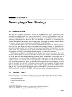
guage, presents a challenge that often requires an ad-hoc solution. The flow in
Figure 12.1 represents a generic co-design methodology.

5

In this diagram, the hard-
ware may be modeled in Verilog, VHDL, or C++ or it could be modeled using field
programmable gate arrays (FPGAs). Specification of the hardware depends on its
purpose. Decisions must be made regarding datapath sizes, number and size of reg-
isters, technology, and so on.

Figure 12.1

Generic co-design methodology.
System specification
Algorithm development
Hardware-software
partitioning
Hardware synthesis Software synthesis
Interface synthesis
System simulation
Design verification System evaluation

Success
?
DONE
yes
no

MEASURING SIMULATION THOROUGHNESS

575

The interface between hardware and software must handle communications
between them. If the model is described in Verilog, running under Unix, then the
Verilog programming language interface (PLI) can communicate with software pro-
cesses using the Unix socket facility. After the design has been verified, system eval-
uation determines whether the system, as partitioned and implemented, satisfies
performance requirements at or under cost objectives. If some aspect of the design
falls short, then another partitioning is performed. This process can be repeated until
objectives are met, or some optimum flow is achieved. Note that if the entire system
is developed using C++, many communications problems are solved, since every-
thing can be compiled and linked as one large executable.

12.4 MEASURING SIMULATION THOROUGHNESS

As indicated previously, many techniques exist for speeding up simulation, thus per-
mitting more stimuli to be applied to a design in a given period of time. However, in
design verification, as in manufacturing test, it is important not to just run a lot of
stimuli, but also to measure the thoroughness of those stimuli. Writing stimuli
blindly, without evaluating their effectiveness, may result in high quantities of low-
quality test stimuli that repeatedly exercise the same functionality. This slows down
the simulations without detecting any new bugs in the design. Coverage analysis can

identify where attention needs to be directed in order to improve thoroughness of the
verification effort. Then, the percentage coverage of the RTL, rather than the quan-
tity of testbench code, becomes the criteria for deciding when to bring design verifi-
cation to a halt.

12.4.1 Coverage Evaluation

Chapter 7 explored a number of topics, including toggle coverage (Section 7.8.4),
gate-level fault simulation (Section 7.5.2), behavioral fault simulation (Section 7.8.3),
and code coverage (Section 7.8.5). Measuring toggle coverage during simulation was
a common practice many years ago. It was appealing because it did not significantly
impact simulation time, nor did it require much memory. However, its appeal for
design verification is rather limited now because it requires a gate-level model. If a
designer simulates at the gate level and finds a bug, it usually becomes necessary to
resynthesize the design, and designers find it inconvenient to interrupt verification
and resynthesize each time a bug is uncovered, particularly in the early stages of
design verification when many bugs are often found in rapid succession. As pointed
out in Section 7.8.4, toggle count remains useful for identifying and correcting hot
spots in a design—that is, areas of a die that experience excessive amounts of logic
activity, causing heat buildup. It was also argued in Chapter 7 that fault simulation
can provide a measure of the thoroughness of design verification vectors. But, like
toggle count, it relies on a gate-level model.
Code coverage has the advantage that it can be used while simulating at the RTL
level. If a bug is found, the RTL is corrected and simulation continues. The RTL is

576

BEHAVIORAL TEST AND VERIFICATION

not synthesized until there is confidence in the correctness of the RTL. As pointed

out in Section 7.8.5, code coverage can be used to measure block coverage, expres-
sion coverage, path coverage, and coverages specific to state machines, such as
branch coverage. When running code coverage, the user can identify modules of
interest and omit those that are not of interest. For example, the logic designer may
include in the design a module pulled down from a library or obtained from a ven-
dor. The module may already have been thoroughly checked out and is currently
being used in other designs, so there is confidence in its design. Hence it can be
omitted from the coverage analysis.
Code coverage measures controllability; that is, it identifies all the states visited
during verification. For example, we are given the equation

WE

=

CS

&

ArraySelect

&

SectorSelect

&

WriteRequest

;

What combinations of the input variables are applied to that expression? Does the
variable

SectorSelect

ever control the response of

WE

? In order for

SectorSelect

to
control

WE

, it must assume the values 0 and 1 while the other three inputs must be
1. For this expression, a code coverage tool can give a coverage percentage, similar
to a fault coverage percentage, indicating how many of the variables have con-
trolled the expression at one time or another during simulation. Block coverage,
which indicates only whether or not a line of code was ever exercised, is a poor
measure of coverage. When verifying logic, it is not uncommon to get the right
response for the wrong reason, what is sometimes referred to as

coincidental cor-
rectness

. For example, two condition code bits in a processor may determine a con-

ditional jump, but the one that triggered the jump may not be the one currently
being investigatated.
Consider the state machine: It is desirable to visit all states, and it is desirable to
traverse all arcs. But, in a typical state machine several variables can control the
state transitions. Given a compound expression that controls the transition from

S

i

to

S

j

, a thorough verification requires that each of the variables, at some point dur-
ing verification, causes or determines the transition to

S

j

. In general, equations can
be evaluated to determine which variables controlled the equation and, more impor-
tantly, which variable never controlled the equation throughout the course of simu-
lation. An important goal of code coverage is to verify that the input vectors
established logic values on internal signals in such a way that the outcome of a
logic transaction depends only on one particular signal, namely, the signal under
consideration.

Behavioral fault simulation, in contrast to code coverage, measures both control-
lability and observability. A fault must be sensitized, and its effects must be propa-
gated to an observable output before it can be counted as detected. One drawback to
behavioral fault simulation is the fact that the industry has never settled on an accept-
able family of faults, in contrast to gate-level fault simulation where stuck-at-1 and
stuck-at-0 faults have been accepted for more than a quarter-century.
Given a fault coverage number estimated using a gate-level model, test engineers
can usually make a reasonably accurate prediction of how many tester escapes to

MEASURING SIMULATION THOROUGHNESS

577

expect from their product lines. So, although the stuck-fault metric is not perfectly
accurate, it is a useful tool for estimating outgoing quality level. Furthermore, many
studies over the years have helped to refine our understanding of the various gate-
level fault models. For example, it is well known that fault models based on stuck-at
faults in gate-level circuits can produce widely divergent results, depending on
which faults are selected and how the fault list is collapsed. Many years ago it was
shown that vectors providing a coverage of 95% for pin faults on SSI and MSI cir-
cuits provided in the neighborhood of 70–75% fault coverage when internal faults
were considered.

6,7

Another drawback to the use of behavioral fault simulation for design verification
is the fact that it only counts as detected those faults that propagate to the output
pins. For design verification, it is frequently unnecessary to propagate behavioral
faults to an output pin, it is sufficient to sensitize (i.e., control) the faults. But, as we
have just seen, code coverage measures controllability, and its metrics are well

understood and accepted. So, if the goal is simply to sensitize logic, then code cov-
erage is adequate.
Another means for determining the thoroughness of coverage is through the use
of event monitors and assertion checkers.

8

The

event monitor

is a block of code that
monitors events in a model in order to determine whether some specific behavior
occurred. For example, did the applied stimuli try to write to a fifo when it was full?
This is a situation that will occur in practice; and in order to determine if the circuit
responds correctly, it is necessary to first verify that this condition occurred and then
verify that the circuit responded as desired. One way to check for this condition is to
write a block of code that checks for “fifo full” and “write enabled.” The code can be
embedded conditionally into a Verilog RTL model using <“ifdef”, “endif”> pairs, or
it can be coded as a standalone module. If the conditions “

fifo_full

” and
“

write_request

” are both found to be true, a message can be written to a log file and
the engineer can then check the circuit response to verify that it is correct.

The

assertion checker

is implemented like an event monitor, but it is used to
detect undesirable or illegal behavior. Consider the case of a circuit that is
required to respond within 50 clock periods to a bus request. This is classified as a
temporal assertion, because the event is required to occur within a specified time
interval, in contrast to the previous example of the fifo, which is classified as a
static event—that is, one in which the events occur simultaneously. It would be
tedious to enumerate all of the possible cases that should be checked during simu-
lation, but many corner cases can be defined and monitored using monitors and
checkers.
Monitors and checkers can supplement code coverage as a means of measur-
ing the thoroughness of a test suite. If there are specific corners of a design that
the designer is interested in, monitors and checkers can explicitly check those
cases. A response from the appropriate checker can put the logic designer’s
mind at ease. It might, however, be argued that if the logic designer used code
coverage and obtained 100% expression coverage, and verified that the circuit
responded correctly for all stimuli, then the designer has already checked the
condition.

578

BEHAVIORAL TEST AND VERIFICATION

Example

Consider the fifo example cited earlier. Somewhere in the logic there may
be an expression similar to the following:

mem_avail

=

fifo_full & write_request

;
In this expression

fifo_full

is high if the fifo is full, and it is low otherwise.

Write_request

goes high if an attempt is made to write to the fifo. If memory is avail-
able,

fifo_full

is low and

mem_avail

is low. However, if an attempt is made to write
to the fifo when it is full,

mem_avail

goes high. If code coverage confirms 100% cov-
erage for this line of code, then all possibilities have been checked. The following is
a table of results that might be printed by a code coverage tool.



These code coverage results indicate that no write requests were attempted when
the fifo was full (count = 0). An advantage of monitors and checkers over code cov-
erage is that they check for specific events that the logic designer is concerned
about, so the designer does not have to scroll through a large file filled with detail. In
addition, code coverage only checks for controllability. The event monitor can be
coded and positioned in the model in such a way as to confirm complete transac-
tions, including events occurring at the memory and at the destinations. However,
regardless of which method is used, in the final analysis the logic designer must
understand the design and verify that the design implements the specification, rather
than his subjective interpretation of the specification.

12.4.2 Design Error Modeling

While the use of behavioral fault simulation for design verification may be of ques-
tionable value, it can be useful for evaluating a manufacturing test suite prior to syn-
thesis. The granularity is more coarse than that of the gate-level model, but it may
nevertheless point to areas of a design where coverage is particularly weak and
where design changes might be helpful. For example, controllability may be quite
poor because long input sequences are needed to reach a particular state, suggesting
that perhaps a parallel load of some counter may be desirable. Perhaps an unused
state in a state machine can be used to load a particular register in test mode in order
to improve controllability. Or this unused state may be used to gate test data out onto
a bus, thus improving observability. By including such changes at the RTL level, in
response to low behavioral fault coverage, the changes can be evaluated and verified

before the circuit is synthesized. Behavioral fault simulation can also be useful in
evaluating diagnostic programs that are intended to be run in the field.
Count

fifo_ full write_request mem_avail

3243 0 1 0
31 0 0
01 1 1
66% Expression coverage


MEASURING SIMULATION THOROUGHNESS

579

In earlier chapters it was noted that if a fault was modeled and detected by a fault
simulator, we can expect it to be detected when the chip is tested. However, fault
simulation cannot say anything about faults that are not modeled. In like manner,
design verification can confirm the correctness of operations that are exercised by
the applied vectors, but it cannot prove the absence of design errors in functions that
were not targeted by the vectors.
This is important to note because, even for very small circuits, the number of
potential errors becomes impractical to consider. In Section 7.7.1 an example was
given wherein, for a simple two-input circuit, 16 possible functions were defined.
For a complex sequential circuit with

n

inputs and

m

internal states, the number of
potential states becomes astronomical very quickly. The task of counting the exact
number of states is further exacerbated by the fact that many of the states are
unreachable in incompletely specified state machines (ISSMs). Furthermore, it is
not immediately obvious how many state transitions are required to reach a given
state from some other, arbitrary state. At best, all we can hope to do is compute an
upper bound on the number of clock cycles required to completely exercise a given
sequential circuit. The reader may recall, from Section 3.4, that these considerations
led early researchers dealing with manufacturing test to introduce the concept of a
stuck-at-fault.
Faster simulation methodologies, such as cycle simulation and point accelera-
tors, have been introduced in order to improve thoroughness of design verification.
In this approach, logic designers keep doing what they have done in the past, but
they do it faster and they do more of it, in the hopes that by using more stimuli
they will be more thorough. The problem with this method is that, like manufac-
turing test programs, if there is no way to evaluate the thoroughness or complete-
ness of the programs, it is possible to quickly reach the point of diminishing
returns: Many thousands of additional vectors are added without improving the
overall thoroughness of the verification effort. Author Boris Beizer calls it the
“pesticide paradox,” wherein insects build up a tolerance for pesticides, and the
continued application of these same pesticides does not remove any more insects
from the fields.

9

The stuck-at model has been an accepted metric for over three decades. While it
is recognized that it is not perfect, it is understood that if stuck-at coverage for a

manufacturing test is 70%, there will be many tester escapes. If stuck-at coverage is
greater than 98%, the number of tester escapes is likely to be very low. Software
analysts have used error seeding to compute a similar number. This involves the
intentional insertion or errors in a design. The design error coverage

C

DE

, analogous
to fault coverage, is
The

C

DE

might be determined by having one group inject design errors and another
independent group write design verification suites. Just as the fault coverage based
C
DE
=
number of errors detected
number of errors injected
* 100%

580

BEHAVIORAL TEST AND VERIFICATION

on stuck-at faults is not perfect, the design error coverage, based on injected faults,
may be either too optimistic or too pessimistic. However, if

C

DE

= 70%, it is a
good idea to keep on writing design verification vectors. If

C

DE

= 100% and if no
bugs have been encountered in some arbitrary interval (e.g., 1 week), then consid-
erable thought must be given to deciding whether the device is ready to be shipped,
recognizing that even if

C

DE

= 100%, it only guarantees that all of the artificially
created and injected design errors were detected, there may still be real errors in
the design.
If error seeding is to be used, it must be decided what kind of errors to inject
into the circuit model. In view of the fact that contemporary circuits are designed
and debugged at the register transfer level, errors should be created and injected
at that level. Like fault simulation, granularity is an issue to consider. Stuck-at

faults can cause detection of gross physical defects in addition to stuck-at faults.
In like manner, gross design errors (e.g., a completely erroneous algorithm imple-
menting arithmetic/logic operations) are likely to be detected by almost any veri-
fication suite, so it makes sense to inject subtle errors that are more difficult to
discover. This includes such things as wrong operators in RTL expressions, incor-
rect variables, or incorrect subscripts. For example, consider the following Ver-
ilog expression:
always @(

sign

or

a

or

b

or

c

or d or e)
g = (!sign) ? a | !(b | c) & d | !e : 0;
If sign is equal to 0, the complex expression is evaluated and its value is assigned to
g; else 0 is assigned to g. Some very simple errors that can be applied to this Verilog
code include leaving out a negation (!) symbol, or placing a left or right parenthesis
in the wrong place, or substituting an OR (|) for an AND (&) or vice versa. One of
the terms might be modified by adding a variable to the product. Sometimes the fail-

ure to include a variable in the sensitivity list, particularly if it is a long list, can
cause a logic designer to puzzle for quite some time over the cause of an erroneous
response in an equation that appears well-formed.
The misuse of blocking and non-blocking assignments in Verilog procedural
statements can cause confusion. Blocking assignments, indicated by the symbol (=),
can suspend, or block, a process until a register is updated. A non-blocking assign-
ment, indicated by the symbol (<=), permits a register to be evaluated, but updated at
a later time, while permitting processing to continue, hence the term non-blocking.
For more complex expressions, such as loop control, error injection can consist
of changing limits, or polarity of a control signal. In case statements intended to rep-
resent state machines, incorrect state machine behavior can be induced by switching
cases. More difficult to detect is the situation where, in one of the cases, a complex
expression is altered. In effect, a good design verification suite should exhaustively
consider all possible values of the variables in a complex expression. This is equiva-
lent to having 100% expression coverage for the expression from a code coverage
tool. Altering the order of the variables in a port list may also provide a good chal-
lenge for a design verification suite.
RANDOM STIMULUS GENERATION
581
If seeding of design errors can be accomplished by a program, similar to fault list
generation for gate-level fault simulation, some of the subjectivity that causes poten-
tial errors to be overlooked can be eliminated. The human may make a judgment as
to whether or not it is necessary to seed a particular part of a design, or to use a par-
ticular error construct. The program, on the other hand, seeds according to some pre-
determined formula. The subjectivity of the design verification process is also a
good reason why a design verification suite is best developed by individuals other
than those who designed the circuit. It also explains why software code inspections
are performed by persons other than those who wrote the software. It is not uncom-
mon for someone who wrote a block of code, whether it be HLL or HDL, to exam-
ine that code several times and not see an obvious error. A similar situation holds for

a specification. The designer may misunderstand some fine point in the specification
and, if he creates stimuli based on this misconception, his simulation results only
confirm that his design functions according to his understanding, which was initially
wrong.
A typical practice when testing S/W is to inject bugs one at a time. After a run
has completed, S/W responses with and without the injected bug are compared. If
the injected bug causes incorrect response, it has been detected. It is not necessary
to debug the circuit since the bug was injected; hence its location is known. Of
course, if the bug escapes detection, then it becomes necessary to determine why it
was not detected. In a regression test, a bug that was previously detected may now
escape detection as a result of a patch inserted to fix another bug. Design error
injection in HDL designs is quite similar to S/W testing. One noticeable difference
is the fact that response of an HDL can be examined at I/O pins. But, recalling our
previous discussion, logic designers may choose not to drive an internal state to an
I/O pin. Hence it may be necessary to capture internal state at registers and state
machines and then output that information to a file where it can be checked for
correctness.
12.5 RANDOM STIMULUS GENERATION
In previous sections we explored methods for simulating faster, so more stimuli
could be evaluated in a given amount of time, and we explored methods for mea-
suring thoroughness of design verification stimuli. A report generated during cover-
age analysis identified modules or functions where coverage was insufficient. We
now turn to stimulus generation. In this section we focus on random stimulus gen-
eration. In subsequent sections, we will explore behavioral automatic test pattern
generation.
One of the purposes of test stimuli created and applied to a design is to give us
confidence in the correctness of the design. The more functionality we verify, the
greater our confidence. Unfortunately, confidence is a subjective thing. We may feel
100% confident in a design that has only been 80% verified! For example, in a sur-
vey, circa 1990, of IC foundries that fault-simulated stimuli provided by their cus-

tomers, it was found that a typical test suite provided by customers yielded
582
BEHAVIORAL TEST AND VERIFICATION
approximately 73% fault coverage for stuck-at faults in the IC. These test suites
were developed during design verification and served as the acceptance test for ICs
provided by the foundry. Part of the reason for low coverage stems from decisions
by logic designers regarding the importance of verifying various parts of the design.
It is not uncommon for a logic designer to make subjective decisions as to which
parts of a design are “complicated” and need to be thoroughly checked out, based on
his or her understanding of the design, versus those parts of the design that are
“straightforward” and need less attention.
Random test pattern generation (RTPG) is frequently used to exercise designs.
Unlike targeted vectors, random vectors distribute stimuli uniformly across the
design, unless some biasing is built into the vectors (cf. Section 9.4.3, weighted ran-
dom patterns).
Given a sufficiently large set of random values and an unbiased set of I/O pins,
each input combination is equally probable. Given a combinational array imple-
menting arithmetic operations, it is often quite easy to create a configuration like
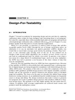
that of Figure 12.2 for an ALU or similar such circuit.
The random pattern generator (RPG) generates a pair of n-wide integers. These
are simulated using the circuit model, but the result is also computed independently
of the simulation. The results are then sent to a comparator that translates the integer
result into binary and compares the two results in order to determine whether the
design responded correctly. The whole process can be automated, and the number of
stimuli applied to the design is limited only by the speed of the simulation process.
A typical stopping rule for such a process is to cease testing when no more errors are
detected after some predetermined number of stimuli have responded correctly.
For sequential circuits, RTPG is a more difficult task because circuit response
depends on current state of the circuit. For example, if a chip-select is disabled, no
amount of stimuli applied to the other input pins will serve a useful purpose until the

chip-select is enabled. Even if the chip-select is enabled, stimuli on other input pins
may be ineffective if an internal control register has not been initialized. But even a
fully initialized circuit may recognize only a small number of input combinations
from its current state. A microprocessor, for example, may be in a state for which
only a single-input combination is useful. Such an example might be a hold or a halt
instruction, for which a controlling state machine only responds to a valid interrupt
request.
Figure 12.2 Applying random stimuli.
RPG Model
Compute
result
Comparator
n
n
integer
integer
RANDOM STIMULUS GENERATION
583
Another complication is the fact that contemporary microprocessors employ mul-
tiple pipelines to decode instructions and allocate resources needed to successfully
execute those instructions. Out-of-order execution of instructions, and contention
for resources by instructions being decoded and executed in parallel pipelines,
means that priorities have to be resolved. If two instructions being decoded in differ-
ent pipelines both require the same general-purpose register, which instruction gets
to use it first? Because of out-of-order execution, an op-code may attempt to per-
form an operation on a register whose value has not yet been set.
Clearly, in these complex processors, it is necessary to exercise every instruction
with all combinations of meaningful data. Load instructions should point at memory
addresses containing valid data. Branch instructions must have valid instructions at
the branch address, and the test must be configured so as to avoid infinite loops.

Conditional branches must be exercised with all condition codes and combinations
of condition codes. Furthermore, it must be verified that branches can be made to
occur, or inhibited, depending on the settings of the condition codes.
Testing the interrupt structure means not just testing for correct operation of
individual interrupts, but also testing to ensure that correct priorities are observed.
If an interrupt is being processed and another interrupt occurs, is the new interrupt
of higher or lower priority than the interrupt currently being processed? If it is of
higher priority, then current interrupt processing must be interrupted, and the new
interrupt must be processed; then the processor must resume processing the inter-
rupt that was originally being processed. In addition to the interrupt inputs, other
input pins must also be exercised at the appropriate times to determine their effect
on the behavior of the design. This includes chip select pins, memory and I/O read
and write pins, and any other pins that are able to affect the flow of control in the
design.
In a program for generating test suites for microprocessors described at the 1982
Design Automation Conference,
10
the various properties of the microprocessor were
systematically captured in a file. This included information about instruction for-
mats, register file sizes, ALU operations, I/O pins, and their effects on the flow of
instructions and data. Details of addressing methods and formats included descrip-
tions of program counters, index registers, stack pointers, and relative and absolute
addressing methods. In addition, information describing controllability and observ-
ability methods of the registers was provided to the system. With this information,
the automatic generation system synthesized sequences of instructions, including
the necessary initialization sequences. Where the system might generate an exces-
sive number of instructions—as, for instance, when generating sequences that test
every register combination for a move register instruction—the user had the option
of selecting a subset adequate to satisfy the objectives of the test.
In another method, whose purpose was to verify the design of an original version

of an IBM System/6000 RISC processor, RTPG was used to make the test program
generation process more productive, comprehensive, and efficient.
11
The system
developed was a dynamic, biased pseudo-random test program generator. Unlike a
so-called static approach where a test program was developed and then simulated in
its entirety, the RTPG system developed by this project was dynamic: Test
584
BEHAVIORAL TEST AND VERIFICATION
generation was interleaved with the execution of instructions. This made it possible
for the logic designer to create test programs during the early stages of design, while
implementing the op-codes.
The test program generated by RTPG is made up of three parts:
Initial state
Instructions
Expected results
The initial state specifies the contents of resources needed to execute a particular
instruction, including registers, flags, and memory contents. Instructions describe
the contents of caches or memory locations. Expected results list the final state of all
resources that were affected by the execution of the instruction. These test programs
are self-contained and include all information required for their independent execu-
tion, so they can migrate between test libraries and they can be executed in any
order.
Example
H 10000:
* A simple test program
R IP 00010000
R R1 03642998
R R8 0000000F
R R10 1E12115F

R R22 0129DFFF
R R30 800000BA
R MSR 00008000
R CR 8CC048C8
R XER 2000CD45
D 0129DFFC 4E74570E
D 03640B90 7D280411
* ------ Assembly Program -------------
I 00010000 7C48F415 a0. R2 .R8.R30
I 00010004 7CD0B02E lx R7 .R0.R22 E/A 0129DFFF
I 00010008 49BBB904 b *+29079812 T/A 01BCB90C
I 01BCB90C B141E1F8 sth R10.X′E1F8′(R1) E/A 03640B90
*------- Expected Results -------------
R IP 01BCB910
R R2 800000C9
R R7 4E74570E
R MSR 00008000
R CR 8CC048C8
RANDOM STIMULUS GENERATION
585
R XER 0000CD45
D 0129DFFC 4E74570E
D 03640B90 115F0411
END 
In this example the header (H) is used to identify the test number. The next line,
starting with an asterisk, denotes a comment. The lines beginning with R denote reg-
isters. The instruction pointer (IP) identifies the start of the test program—in this
case, hex location 10,000. The data entries (D) define memory locations and the data
stored at those locations. The instruction (I) entries identify memory addresses and
the instructions to be saved at those locations. Note that the first three instructions

are contiguous, and then the fourth entry is some distance away from the previous
three. The instructions contain assembly code for documentation purposes. In this
sequence, the instructions sequence contains add, load, branch, and store instruc-
tions. The third instruction causes a branch to location 01BCB90C, where the store
instruction is located.
The short program in this example can be executed as soon as all of the instruc-
tions used in the example have been implemented. The RTPG initializes the registers
used by the instructions being tested, so it is not necessary to employ load and store
instructions. The RTL language used for this project was APL (a programming lan-
guage), and the tools are in-house proprietary tools. The test is constructed dynami-
cally, meaning that for each instruction there is a generation stage and an execution
stage. During the generation stage an instruction is chosen and required resources
are initialized. The execution stage is then invoked to execute the instruction and
update affected resources.
Biasing is used in this system to increase the probability of occurrence of events
that might otherwise not occur. Biasing directs the generation process toward
selected design areas so that most events are tested when the number of test pro-
grams is reasonably large. Biasing functions are used to influence the selection of
instructions, instruction fields, registers, addresses, data, and other components that
go into construction of a test program. Each instruction or process, such as an inter-
rupt or address translation, is represented by a block diagram composed of decision
and execution blocks. In every decision block the data affecting the decision are
selected in such a way that subsequent blocks are entered with user-specified or
RTPG controlled probability. As an example, the user may request that there be a
10% probability that the arguments selected for a floating point operation produce
an overflow.
The biasing functions evolve over a number of projects, so weaknesses observed
in the RTPG can be corrected by altering the probabilities; consequently, the func-
tions can be influenced by those probabilities. Code coverage techniques can be
used to evaluate the behavior of RTPG; and, by identifying weaknesses, such as

lines of code not touched by the RTPG, the results of code coverage can be used to
improve the biasing functions. Biasing can also be improved by analyzing the
effects of fault injection. Faults or design errors are injected into the model, and it is
determined whether or not they are detected by any randomly generated test
586
BEHAVIORAL TEST AND VERIFICATION
program. If, at the conclusion of the design verification effort, there are injected
errors that went undetected, then either the biasing functions need to be refined, or,
perhaps, the circuit requires a greater number of test programs in order to detect all
errors.
In yet another project employing RTPG, the object of the effort was a multipro-
cessor workstation cache controller.
12
The workstations can contain up to 12 proces-
sor boards, with each processor board containing three custom VLSI chips and a
128-kbyte cache memory. Main memory is shared among the workstations. One of
the chips is a cache controller whose purpose is to make memory transparent to the
processors. It manages the cache and communicates with main memory and periph-
erals. It consists of a processor cache controller (PCC) and a snooping bus controller
(SBC). Each of these two subsystems is complex in and of itself, with many states
and transitions. When interactions between PCC and SBC are considered, there are
many thousands of possible interactions.
Although the object of this verification effort was to verify the cache controller,
it was believed that simulating the cache controller by itself would not be sufficient
to verify the system’s design. So, the simulation model consisted of all three chips,
the cache controller, the CPU, and the floating-point coprocessor. However, for the
random tester, a stub module replaced the CPU, simplified inside but accurately
modeling the interface. This model was easier to write than a full model, it allowed
for more flexible timing, and it ran faster than a full model. Three copies of the
three-chip workstation model were instantiated in order to verify the memory

design.
The stub CPU generated memory references by randomly selecting from a pre-
determined script. The scripts, an example of which is illustrated in Figure 12.3,
consist of action/check pairs, in which the action produces a state change and the
check verifies that the change happened correctly. For example, an action might
write a particular value to a memory address. The corresponding check verifies that
the update occurred correctly, or signals an error if it did not. Because of the random
sequencing, an arbitrary amount of time and a random permutation of other actions
and checks may elapse between an action and its corresponding check.
Figure 12.3 Action/check pair.
CacheOp Address Data Mode
Action
Write32 0x00000660 0x05050505 User
Check
Read32 0x00000660 0x05050505 Kernel
Write32 0x00000660 0x05050505 Kernel
End
Action
TestSet 0x0000A800 0x0 User
Check
Read32 0x0000A800 0x1 User
Write32 0x0000A800 0x0 User
End
THE BEHAVIORAL ATPG
587
In Figure 12.3 the words Action, Check, and End are keywords that delineate an
action/check pair. An entry identifies a cache operation, the cache address, the data
to be written to or read from that address, and the mode. Reserved data words can be
used to instruct the CPU to expect specific exception conditions, such as a page
fault, to occur. In the second action/check pair, the TestSet cache operation expects

the current value at address 0x0000A800 to be 0. It then sets the value to 1. A check
performed later expects a 1, and then it clears the value so the next execution of the
action will find a 0.
The RTPG was determined by its implementers and users to be a major success.
Before it was implemented, several months were spent writing design verification
tests in assembly language. These tests covered about half of the uniprocessor cases
and none of the multiprocessor cases. The initial version of the random tester, writ-
ten in a week, immediately revealed numerous errors, including significant design
problems. The final version of the RTPG required about two months and detected
over half the bugs uncovered during functional verification. The strategy devised for
the RTPG was to run until it uncovered a problem, or forever if it could not find any.
During the early stages the RTPG would run for about 20 minutes on a Sun3/160
workstation. By the end of verification, it had run continuously for two weeks on
multiple computers, using different random seeds.
12.6 THE BEHAVIORAL ATPG
The goal of behavioral ATPG (BATG) is to exploit knowledge inherent in RTL and
behavioral level circuit descriptions. ATPG programs have traditionally relied on
gate-level circuit descriptions; as circuits grew larger, the ATPGs frequently became
entangled in a myriad of details. Managing gate-level descriptions for larger circuits
requires exorbitant amounts of memory and CPU time. By exploiting behavior
rather than structure, and taking advantage of higher levels of abstraction, the
amount of detail is reduced, permitting more efficient operation. Perhaps more
importantly, it is possible to distinguish between legal and illegal behaviors of state
machines, handshaking protocols, and other functions. It is possible to recognize
state-space solutions that would be next to impossible to recognize at the gate level.
In addition, it becomes possible to recognize when a solution does not exist, and
cease exploring that path.
12.6.1 Overview
A simple example of a circuit where behavioral knowledge can be used to advantage
is the one-hot encoding of a state machine (see, for example, Figure 9.30). A gate-

level ATPG, attempting to justify an assignment to the state machine, may spend
countless hours of CPU time trying to justify a logic 1 on two or more flip-flops
when the implementation only permits a single flip-flop to be at logic 1 at any given
time. By abstracting out details and explicitly identifying legal behavior of the state
machine, this difficulty can be avoided.
588
BEHAVIORAL TEST AND VERIFICATION
In other cases the amount of CPU time required to generate a test at the gate
level, even when a test exists, is prohibitive. A circuit as basic as an 8-bit binary
counter, capable of counting from 0 to 255, can frustrate an ATPG, since it may
require as many as 256 time frames to propagate or justify primitive D-cubes of fail-
ure (PDCF). In combinational logic a 64- or 80-bit array multiplier represents a sig-
nificant challenge to a combinational ATPG, even though theory assures us
(Section 4.3) that the ATPG, if allowed to run indefinitely, will eventually find a
solution. Note that incremental improvements in ATPG performance have been real-
ized by introducing slightly larger primitives, such as 2-to-1 multiplexers and
adders, as primitives. This is a rather small concession to the need for a higher level
of modeling.
12.6.2 The RTL Circuit Image
Chapter 2 introduced a circuit model in the form of a graph in which nodes corre-
sponded to individual logic elements and arcs corresponded to connections
between elements. The nodes were represented by descripter cells containing point-
ers and other data (see Figure 2.21). The pointers described I/O connections
between the output of one element and the inputs of other elements. The ATPG
used the pointers to traverse a circuit, tracing through the interconnections in order
to propagate logic values forward to primary outputs and justify assignments back
toward the inputs.
For logic elements in an RTL circuit the descripter cells bear a similarity, but
functions of greater complexity require more entries in the descripter cell. In addi-
tion, linking elements via pointers is more complex. In gate-level circuits the

inputs of logic gates are identical in function, but in RTL circuits the inputs may
be busses and can serve much more complicated functions. The circuit in
Figure 12.4 represents a generic view of a function. It is characterized by the fact
that its inputs are control and data ports, and its outputs are status and data ports.
Furthermore, each of its ports may be n
i
bits wide (n
i
≥ 1) and, when n
i
> 1, it is
important to indicate whether the high-order bit is numbered bit 0 or bit n
i
− 1.
Not shown in this generic model are internal registers. The registers may hold data
or control bits.
Figure 12.4 Generic representation of a function.
n
1
n
i
m
j
T
c
m
1
Status
Control
s

THE BEHAVIORAL ATPG
589
In in the case of a 2-to-1 multiplexer the control could require one or two inputs.
One control bit selects one of two data inputs, and the other control bit, if present,
enables the output. If the output is disabled, it may be floating (Z state), or forced to
a 1 or 0. In the case of an ALU, an operation may require one of several functions to
be chosen, thus requiring several control bits. A connectivity graph must embrace all
of this information in some orderly way that can be used by many software routines.
When a gate-level ATPG program is implemented, one of the first questions that
must be addressed is that of support for primitives. What primitives will the ATPG
support? Will the knowledge for these primitives be built into the ATPG, or will that
knowledge be represented in tabular form? For example, an AND gate is a primitive
for which the ATPG has processing capability. The ATPG may have a routine that
simply retrieves the input count for the AND gate and then loops on input values in
order to compute the output. When justifying a 0 on the output, it selects one of the
inputs and assigns a 0 to the gate driving that input. When propagating through an
input, the ATPG knows that it must justify 1s on all the other inputs.
An alternate approach is to employ a truth table, from which PDCFs and other
information can be compiled and retrieved as needed (see Section 4.3). An advantage
of this is that new primitives can be easily supported simply by adding the appropri-
ate truth table whenever it is advantageous to do so. For example, if a circuit contains
many 2-to-1 multiplexers, it may be advantageous to represent the multiplexer as a
single primitive, rather than as several logic gates. A standard cell library may have
an ATPG model for the multiplexer. When backtracing the 2-to-1 multiplexer using
the truth table, the ATPG tries to find an entry in the table that is compatible with the
existing state of the circuit. There is no explicit awareness that the multiplexer is
making a choice, by way of its control input, from one of two inputs D
0
or D
1

.
12.6.3 The Library of Parameterized Modules
For RTL functions, not only are data structures more complex, but processing is also
more complex. The types of functions is seemingly endless. How is it possible to
create something analogous to a gate-level ATPG? One way to control the scope of
the problem is to require that a behavioral ATPG restrict itself to synthesizable cir-
cuits. Another way to reduce the scope of the problem, when parsing an RTL circuit,
is to identify basic functions and map these into canonical forms. Then the intercon-
nection of these elements is accomplished through pointers, just as is done at the
gate level. A logical question to ask is, “How many basic functions are there?” The
Electronic Design Interchange Format (EDIF) webpage
13
contains a Library of
Parameterized Functions (LPM), which lists 25 basic functions:
CONST INV AND OR XOR
LATCH FF SHIFTREG RAM_DQ RAM_IO
ROM DECODE MUX CLSHIFT COMPARE
ADD_SUB MULTIPLER COUNTER ABS BUSTRI
FSM TTABLE INPAD OUTPAD BIPAD
590
BEHAVIORAL TEST AND VERIFICATION
Some of these are obvious, others are not so obvious. The CONST model returns a
constant value. CLSHIFT is a combinatorial shifter. RAM_IO has a bidirectional
data port, while RAM_DQ has an input data port and an output data port. TTABLE
is a truth table and FSM is a finite-state machine.
Each of these entries is characterized by a number of parameters. The following
are some of the properties that characterize COUNTER:
Counter width
Direction (up, down, or dynamic)
Enable (clock or count)

Load style (synchronous or asynchronous)
Load data (variable or constant)
Set or clear (synchronous or asynchronous)
If dynamic count is specified, then the direction of count, up or down, is under con-
trol of an input pin. There are other properties that need to be considered. For exam-
ple, the width of the counter may be eight bits, but the maximum count of the
counter may be less than 2
width
. If a data structure exists for COUNTER that sup-
ports all of the LPM properties, then a counter that appears in an RTL description
can be represented by that data structure. If a particular property does not appear in
the RTL description, then that field in the data structure is either left blank or set to a
default value. A particular counter in a circuit may have a load capability but may
not have a set or clear. In such a case the counter can be loaded with an all-0s or all-
1s value to implement the set or clear operation.
Some of the entries, including the truth table, the finite-state machine, and the
RAM and ROM modules do not have a standard size. A RAM may be a small bank
of registers, or it could be a large cache memory. So, in addition to holding parame-
ters that characterize functionality of these devices, the data structure will need to
have variably sized data fields that hold the actual data. Memory for a truth table and
transition tables for an FSM can be allocated while the circuit model is being con-
structed, but memory for the RAM and ROM may have to be allocated dynamically.
Recognizing the presence of an LPM function in an RTL circuit description is
accomplished by recognizing keywords and commonly occurring expressions. In
Verilog the posedge and negedge keywords identify flip-flops. A case statement
could represent a multiplexer, or it could represent a state machine (cf. Figure 9.30).
The presence of posedge or negedge helps to distinguish between the multiplexer
and state machine. A construct such as a counter is detected by observing the
counter being incremented or decremented by a constant value. The b16ctr model, a
16-bit counter (see also Section 7.8.2), illustrates the increment operation.

module b16ctr(ctrout,din,clk,loadall,incrcntr,
decrcntr,rst);
parameter width = 32;
output [width-1:0] ctrout;
THE BEHAVIORAL ATPG
591
input [width-1:0] din;
input clk, rst, loadall, incrcntr, decrcntr;
reg [width-1:0] ctrout;
wire load = loadall & rst;
always @(posedge clk) begin
if(!load)
ctrout <= din;
else if(incrcntr | decrcntr)
ctrout <= (decrcntr) ? ctrout - 1 : ctrout + 1;
end
endmodule
The data width is set to 32, but it can be overridden by the invoking module, so
this model could represent a counter of any size. This example always increments or
decrements by 1. The increment value could also be a parameter or variable. For
example, if this were a program counter, the increment value might be 1, 2, or 4,
depending on whether it is incrementing by one byte, a 16-bit word, or a double
word. Also it must be noted that a set or reset input may be active low or active high.
The clock also may be positive- or negative-edge triggered. These distinctions must
be noted and recorded as part of the characterization of the counter.
An if ... else construct indicates the presence of a multiplexer. The following Ver-
ilog expression describes a 2:1 multiplexer:
wire outx = (sel == 1) ? A : B;
If the multiplexer has more than two choices, it might be expressed by means of a
case statement. A decoder can also use a case statement. A typical decoder expres-

sion may appear as follows:
case ({I1,I0})
2′b11: Y[3:0] = 4′b1000;
2′b10: Y[3:0] = 4′b0100;
2′b01: Y[3:0] = 4′b0010;
2′b00: Y[3:0] = 4′b0001;
endcase;
When a behavioral ATPG parses an RTL model and associates RTL constructs
with logic functions, the actions are similar to those performed during logic synthe-
sis. The major difference lies in what must be done after the RTL description has
been parsed. Whereas synthesis software is simply concerned with mapping an RTL
description into a gate-level equivalent, using a standard cell library or some similar
such target representation, and performing some minimizations along the way,
BATG must understand the behavior of the RTL constructs that it encounters. It