Tài liệu Microstrip bộ lọc cho các ứng dụng lò vi sóng RF (P8) doc
Bạn đang xem bản rút gọn của tài liệu. Xem và tải ngay bản đầy đủ của tài liệu tại đây (528.7 KB, 38 trang )
CHAPTER 8
Coupled Resonator Circuits
Coupled resonator circuits are of importance for design of RF/microwave filters, in
particular the narrow-band bandpass filters that play a significant role in many ap-
plications. There is a general technique for designing coupled resonator filters in the
sense that it can be applied to any type of resonator despite its physical structure. It
has been applied to the design of waveguide filters [1–2], dielectric resonator filters
[3], ceramic combline filters [4], microstrip filters [5–7], superconducting filters
[8], and micromachined filters [9]. This design method is based on coupling coeffi-
cients of intercoupled resonators and the external quality factors of the input and
output resonators. We actually saw some examples in Chapter 5 when we discussed
the design of hairpin-resonator filters and combline filters, and we will discuss
more applications for designing various filters through the remainder of this book.
Since this design technique is so useful and flexible, it would be desirable to have a
deep understanding not only of its approach, but also its theory. For this purpose,
this chapter will present a comprehensive treatment of the relevant subjects.
The general coupling matrix is of importance for representing a wide range of
coupled-resonator filter topologies. Section 8.1 shows how it can be formulated ei-
ther from a set of loop equations or from a set of node equations. This leads to a
very useful formula for analysis and synthesis of coupled-resonator filter circuits in
terms of coupling coefficients and external quality factors. Section 8.2 considers
the general theory of couplings in order to establish the relationship between the
coupling coefficient and the physical structure of synchronously or asynchronously
tuned coupled resonators. Following this, a discussion of a general formulation for
extracting coupling coefficients is given in Section 8.3. Formulations for extracting
the external quality factors from frequency responses of the externally loaded in-
put/output resonators are derived in Section 8.4. The final section of this chapter de-
scribes some numerical examples to demonstrate how the formulations obtained
can be applied to extract coupling coefficients and external quality factors of mi-
crowave coupling structures from EM simulations.
235
Microstrip Filters for RF/Microwave Applications. Jia-Sheng Hong, M. J. Lancaster
Copyright © 2001 John Wiley & Sons, Inc.
ISBNs: 0-471-38877-7 (Hardback); 0-471-22161-9 (Electronic)
8.1 GENERAL COUPLING MATRIX FOR COUPLED-RESONATOR FILTERS
8.1.1 Loop Equation Formulation
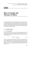
Shown in Figure 8.1(a) is an equivalent circuit of n-coupled resonators, where L, C,
and R denote the inductance, capacitance, and resistance, respectively; i represents
the loop current; and e
s
the voltage source. Using the voltage law, which is one of
Kirchhoff’s two circuit laws and states that the algebraic sum of the voltage drops
around any closed path in a network is zero, we can write down the loop equations
for the circuit of Figure 8.1(a)
R
1
+ j
L
1
+
i
1
– j
L
12
i
2
··· – j
L
1n
i
n
= e
s
– j
L
21
i
1
+
j
L
2
+
ᎏ
j
1
C
2
ᎏ
i
2
··· – j
L
2n
i
n
= 0
(8.1)
Ӈ
– j
L
n1
i
1
– j
L
n2
i
2
··· +
R
n
+ j
L
n
+
i
n
= 0
in which L
ij
= L
ji
represents the mutual inductance between resonators i and j, and
the all loop currents are supposed to have the same direction as shown in Figure
8.1(a), so that the voltage drops due to the mutual inductance have a negative sign.
This set of equations can be represented in matrix form
1
ᎏ
j
C
n
1
ᎏ
j
C
1
236
COUPLED RESONATOR CIRCUITS
L
2
i
2
C
2
L
n-1
i
n-1
C
n-1
L
1
i
1
C
1
R
1
R
1
R
n
e
s
e
s
L
n
i
n
C
n
R
n
()
a
()
b
Two-port n-coupled
resonator filter
V
1
V
2
I
1
I
2
a
1
a
2
b
1
b
2
FIGURE 8.1 (a) Equivalent circuit of n-coupled resonators for loop-equation formulation. (b) Its net-
work representation.
8.1 GENERAL COUPLING MATRIX FOR COUPLED-RESONATOR FILTERS
237
R
1
+ j
L
1
+
ᎏ
j
1
C
1
ᎏ
–j
L
12
··· –j
L
1n
–j
L
21
j
L
2
+
ᎏ
j
1
C
2
ᎏ
··· –j
L
2n
΄΅
΄΅
=
΄΅
(8.2)
ӇӇӇӇ
–j
L
n1
–j
L
n2
··· R
n
+ j
L
n
+
ᎏ
j
1
C
n
ᎏ
or
[Z]·[i] = [e]
where [Z] is an n × n impedance matrix.
For simplicity, let us first consider a synchronously tuned filter. In this case, the
all resonators resonate at the same frequency, namely the midband frequency of fil-
ter
0
= 1/
͙
L
ෆ
C
ෆ
, where L = L
1
= L
2
= ··· L
n
and C = C
1
= C
2
= ··· C
n
. The imped-
ance matrix in (8.2) may be expressed by
[Z] =
0
L·FBW·[Z
ෆ
] (8.3)
where FBW = ⌬
/
0
is the fractional bandwidth of filter, and [Z
ෆ
] is the normalized
impedance matrix, which in the case of synchronously tuned filter is given by
ᎏ
0
L
R
·F
1
BW
ᎏ
+ p –j
ᎏ
0
ᎏ
ᎏ
L
L
12
ᎏ
·
ᎏ
FB
1
W
ᎏ
··· –j
ᎏ
0
ᎏ
ᎏ
L
L
1n
ᎏ
·
ᎏ
FB
1
W
ᎏ
–j
ᎏ
0
ᎏ
ᎏ
L
L
21
ᎏ
·
ᎏ
FB
1
W
ᎏ
p ··· –j
ᎏ
0
ᎏ
ᎏ
L
L
2n
ᎏ
·
ᎏ
FB
1
W
ᎏ
[Z
ෆ
] =
΄΅
(8.4)
ӇӇӇӇ
–j
ᎏ
0
ᎏ
ᎏ
L
L
n1
ᎏ
·
ᎏ
FB
1
W
ᎏ
–j
ᎏ
0
ᎏ
ᎏ
L
L
n2
ᎏ
·
ᎏ
FB
1
W
ᎏ
···
ᎏ
0
L
R
·F
n
BW
ᎏ
+ p
with
p = j
–
the complex lowpass frequency variable. It should be noticed that
= for i = 1, n (8.5)
1
ᎏ
Q
ei
R
i
ᎏ
0
L
0
ᎏ
ᎏ
0
1
ᎏ
FBW
e
s
0
Ӈ
0
i
1
i
2
Ӈ
i
n
Q
e1
and Q
en
are the external quality factors of the input and output resonators, re-
spectively. Defining the coupling coefficient as
M
ij
= (8.6)
and assuming
/
0
Ϸ 1 for a narrow-band approximation, we can simplify (8.4) as
ᎏ
q
1
e1
ᎏ
+ p –jm
12
··· –jm
1n
–jm
21
p ··· –jm
2n
[Z
ෆ
] =
΄΅
(8.7)
ӇӇӇӇ
–jm
n1
–jm
n2
···
ᎏ
q
1
en
ᎏ
+ p
where q
e1
and q
en
are the scaled external quality factors
q
ei
= Q
ei
· FBW for i = 1, n (8.8)
and m
ij
denotes the so-called normalized coupling coefficient
m
ij
= (8.9)
A network representation of the circuit of Figure 8.1(a) is shown in Figure 8.1(b),
where V
1
, V
2
and I
1
, I
2
are the voltage and current variables at the filter ports, and
the wave variables are denoted by a
1
, a
2
, b
1
, and b
2
. By inspecting the circuit of Fig-
ure 8.1(a) and the network of Figure 8.1(b), it can be identified that I
1
= i
1
, I
2
= –i
n
,
and V
1
= e
s
– i
1
R
1
. Referring to Chapter 2, we have
a
1
=
ᎏ
2
͙
e
s
R
ෆ
1
ෆ
ᎏ
b
1
=
(8.10)
a
2
= 0 b
2
= i
n
͙
R
ෆ
n
ෆ
and hence
S
21
=
Έ
a
2
=0
=
(8.11)
S
11
=
Έ
a
2
=0
= 1 –
2R
1
i
1
ᎏ
e
s
b
1
ᎏ
a
1
2
͙
R
ෆ
1
R
ෆ
n
ෆ
i
n
ᎏᎏ
e
s
b
2
ᎏ
a
1
e
s
– 2i
1
R
1
ᎏ
2͙R
ෆ
1
ෆ
M
ij
ᎏ
FBW
L
ij
ᎏ
L
238
COUPLED RESONATOR CIRCUITS
Solving (8.2) for i
1
and i
n
, we obtained
i
1
=
ᎏ
0
L·
e
F
s
BW
ᎏ
[Z
ෆ
]
11
–1
(8.12)
i
n
=
ᎏ
0
L·
e
F
s
BW
ᎏ
[Z
ෆ
]
n1
–1
where [Z
ෆ
]
ij
–1
denotes the ith row and jth column element of [Z
ෆ
]
–1
. Substituting (8.12)
into (8.11) yields
S
21
=
ᎏ
2
0
͙
L·
R
ෆ
F
1
B
R
ෆ
W
n
ෆ
ᎏ
[Z
ෆ
]
n1
–1
S
11
= 1 –
ᎏ
0
L
2
·
R
F
1
BW
ᎏ
[Z
ෆ
]
11
–1
Recalling the external quality factors defined in (8.5) and (8.8), we have
S
21
= 2
ᎏ
͙
q
ෆ
e
1
1
ෆ
·q
ෆ
en
ෆ
ᎏ
[Z
ෆ
]
n1
–1
(8.13)
S
11
= 1 –
ᎏ
q
2
e1
ᎏ
[Z
ෆ
]
11
–1
In the case that the coupled-resonator circuit of Figure 8.1 is asynchronously
tuned, and the resonant frequency of each resonator, which may be different, is
given by
0i
= 1/
͙
L
ෆ
i
C
ෆ
i
ෆ
, the coupling coefficient of asynchronously tuned filter is
defined as
M
ij
= for i
j (8.14)
It can be shown that (8.7) becomes
ᎏ
q
1
e1
ᎏ
+ p – jm
11
–jm
12
··· –jm
1n
–jm
21
p – jm
22
··· –jm
2n
[Z
ෆ
] =
΄΅
(8.15)
ӇӇӇӇ
–jm
n1
–jm
n2
···
ᎏ
q
1
en
ᎏ
+ p – jm
nn
The normalized impedance matrix of (8.15) is almost identical to (8.7) except that it
has the extra entries m
ii
to account for asynchronous tuning.
L
ij
ᎏ
͙
L
ෆ
i
L
ෆ
j
ෆ
8.1 GENERAL COUPLING MATRIX FOR COUPLED-RESONATOR FILTERS
239
8.1.2 Node Equation Formulation
As can be seen, the coupling coefficients introduced in the above section are all
based on mutual inductance, and hence the associated couplings are magnetic cou-
plings. What formulation of the coupling coefficients would result from a two-port
n-coupled resonator filter with electric couplings? We may find the answer to the
dual basis directly. However, let us consider the n-coupled resonator circuit shown
in Figure 8.2(a), where v
i
denotes the node voltage, G represents the conductance,
and i
s
is the source current. According to the current law, which is the other one of
Kirchhoff’s two circuit laws and states that the algebraic sum of the currents leaving
a node in a network is zero, with a driving or external current of i
s
the node equa-
tions for the circuit of Figure 8.2(a) are
G
1
+ j
C
1
+
v
1
– j
C
12
v
2
··· – j
C
1n
v
n
= i
s
– j
C
21
v
1
+
j
C
2
+
ᎏ
j
1
L
2
ᎏ
v
2
··· – j
C
2n
v
n
= 0
(8.16)
Ӈ
– j
C
n1
v
1
– j
C
n2
v
2
··· +
G
n
+ j
C
n
+
ᎏ
j
1
L
n
ᎏ
v
n
= 0
where C
ij
= C
ji
represents the mutual capacitance across resonators i and j. Note that
all node voltages are with respect to the reference node (ground), so that the cur-
1
ᎏ
j
L
1
240
COUPLED RESONATOR CIRCUITS
L
2
v
2
C
2
L
n-1
v
n-1
C
n-1
L
1
v
1
C
1
G
1
G
1
i
s
i
s
L
n
v
n
C
n
G
n
G
n
()a
()b
Two-port n-coupled
resonator filter
V
1
V
2
I
1
I
2
a
1
a
2
b
1
b
2
FIGURE 8.2 (a) Equivalent circuit of n-coupled resonators for node-equation formulation. (b) Its net-
work representation.
rents resulting from the mutual capacitance have a negative sign. Arrange this set of
equations in matrix form
G
1
+ j
C
1
+
ᎏ
j
1
L
1
ᎏ
–j
C
12
··· –j
C
1n
–j
C
21
j
C
2
+
ᎏ
j
1
L
2
ᎏ
··· –j
C
2n
΄΅
΄΅
=
΄΅
(8.17)
ӇӇӇӇ
–j
C
n1
–j
C
n2
··· G
n
+ j
C
n
+
ᎏ
j
1
L
n
ᎏ
or
[Y]·[v] = [i]
in which [Y] is an n × n admittance matrix.
Similarly, the admittance matrix in (8.17) may be expressed by
[Y] =
0
C·FBW·[Y
ෆ
] (8.18)
where
0
= 1/
͙
L
ෆ
C
ෆ
is the midband frequency of filter, FBW = ⌬
/
0
is the frac-
tional bandwidth, and [Y
ෆ
] is the normalized admittance matrix. In the case of syn-
chronously tuned filter, [Y
ෆ
] is given by
ᎏ
0
C
G
·F
1
BW
ᎏ
+ p –j
ᎏ
0
ᎏ
ᎏ
C
C
12
ᎏ
·
ᎏ
FB
1
W
ᎏ
··· –j
ᎏ
0
ᎏ
ᎏ
C
C
1n
ᎏ
·
ᎏ
FB
1
W
ᎏ
–j
ᎏ
0
ᎏ
ᎏ
C
C
21
ᎏ
·
ᎏ
FB
1
W
ᎏ
p ··· –j
ᎏ
0
ᎏ
ᎏ
C
C
2n
ᎏ
·
ᎏ
FB
1
W
ᎏ
[Y
ෆ
] =
΄΅
(8.19)
ӇӇӇӇ
–j
ᎏ
0
ᎏ
ᎏ
C
C
n1
ᎏ
·
ᎏ
FB
1
W
ᎏ
–j
ᎏ
0
ᎏ
ᎏ
C
C
n2
ᎏ
·
ᎏ
FB
1
W
ᎏ
···
ᎏ
0
C
G
·F
n
BW
ᎏ
+ p
where p the complex lowpass frequency variable. Notice that
= for i = 1, n (8.20)
with Q
e
being the external quality factor. Let us define the coupling coefficient
M
ij
= (8.21)
C
ij
ᎏ
C
1
ᎏ
Q
ei
G
i
ᎏ
0
C
i
s
0
Ӈ
0
v
1
v
2
Ӈ
v
n
8.1 GENERAL COUPLING MATRIX FOR COUPLED-RESONATOR FILTERS
241
and assume
/
0
Ϸ 1 for the narrow-band approximation. A simpler expression of
(8.19) is obtained:
ᎏ
q
1
e1
ᎏ
+ p –jm
12
··· –jm
1n
–jm
21
p ··· –jm
2n
[Y
ෆ
] =
΄΅
(8.22)
ӇӇӇӇ
–jm
n1
–jm
n2
···
ᎏ
q
1
en
ᎏ
+ p
where q
ei
and m
ij
denote the scaled external quality factor and normalized coupling
coefficient defined by (8.8) and (8.9), respectively.
Similarly, it can be shown that if the coupled-resonator circuit of Figure 8.2(a) is
asynchronously tuned, (8.21) and (8.22) become
M
ij
= for i j (8.23)
ᎏ
q
1
e1
ᎏ
+ p – jm
11
–jm
12
··· –jm
1n
–jm
21
p – jm
22
··· –jm
2n
[Y
ෆ
] =
΄΅
(8.24)
ӇӇӇӇ
–jm
n1
–jm
n2
···
ᎏ
q
1
en
ᎏ
+ p – jm
nn
To derive the two-port S-parameters of a coupled-resonator filter, the circuit of Fig-
ure 8.2(a) is represented by a two-port network of Figure 8.2(b), where the all vari-
ables at the filter ports are the same as those in Figure 8.1(b). In this case, V
1
= v
1
,
V
2
= v
n
and I
1
= i
s
– v
1
G
1
. We have
a
1
=
ᎏ
2
͙
i
s
G
ෆ
1
ෆ
ᎏ
b
1
=
(8.25)
a
2
=0 b
2
= v
n
͙
G
ෆ
n
ෆ
S
21
=
ᎏ
b
a
2
1
ᎏ
Έ
a
2
=0
=
(8.26)
S
11
=
ᎏ
b
a
1
1
ᎏ
Έ
a
2
=0
=
ᎏ
2v
i
1
s
G
1
ᎏ
– 1
2͙G
ෆ
1
G
ෆ
n
ෆ
v
n
ᎏᎏ
i
s
2v
1
G
1
– i
s
ᎏᎏ
2͙G
ෆ
1
ෆ
C
ij
ᎏ
͙
C
ෆ
i
C
ෆ
j
ෆ
242
COUPLED RESONATOR CIRCUITS
Finding the unknown node voltages v
1
and v
n
from (8.17)
v
1
=
ᎏ
0
C·
i
F
s
BW
ᎏ
[Y
ෆ
]
11
–1
(8.27)
v
n
=
ᎏ
0
C·
i
F
s
BW
ᎏ
[Y
ෆ
]
n1
–1
where [Y
ෆ
]
ij
–1
denotes the iith row and jth column element of [Y
ෆ
]
–1
. Replacing the
node voltages in (8.26) with those given by (8.27) results in
S
21
=
ᎏ
2
0
͙
C
G
ෆ
·F
1
B
G
ෆ
W
n
ෆ
ᎏ
[Y
ෆ
]
n1
–1
(8.28)
S
11
=
ᎏ
0
C
2
·
G
F
1
BW
ᎏ
[Y
ෆ
]
11
–1
– 1
which can be simplified as
S
21
= 2
ᎏ
͙
q
ෆ
e
1
1
ෆ
·q
ෆ
en
ෆ
ᎏ
[Y
ෆ
]
n1
–1
(8.29)
S
11
=
ᎏ
q
2
e1
ᎏ
[Y
ෆ
]
11
–1
– 1
8.1.3 General Coupling Matrix
In the foregoing formulations, the most notable thing is that the formulation of nor-
malized impedance matrix [Z
ෆ
] is identical to that of normalized admittance matrix
[Y
ෆ
]. This is very important because it implies that we could have a unified formula-
tion for a n-coupled resonator filter regardless of whether the couplings are magnet-
ic or electric or even the combination of both. Accordingly, the equations of (8.13)
and (8.29) may be incorporated into a general one:
S
21
= 2
ᎏ
͙
q
ෆ
e
1
1
ෆ
·q
ෆ
en
ෆ
ᎏ
[A]
n1
–1
(8.30)
S
11
= ±
1 –
ᎏ
q
2
e1
ᎏ
[A]
11
–1
with
[A] = [q] + p[U] – j[m]
where [U] is the n × n unit or identity matrix, [q] is an n × n matrix with all entries
zero, except for q
11
= 1/q
e1
and q
nn
= 1/q
en
, [m] is the so-called general coupling ma-
8.1 GENERAL COUPLING MATRIX FOR COUPLED-RESONATOR FILTERS
243
trix, which is an n × n reciprocal matrix (i.e., m
ij
= m
ji
) and is allowed to have
nonzero diagonal entries m
ii
for an asynchronously tuned filter.
For a given filtering characteristic of S
21
(p) and S
11
(p), the coupling matrix and
the external quality factors may be obtained using the synthesis procedure devel-
oped in [10–11]. However, the elements of the coupling matrix [m] that emerge
from the synthesis procedure will, in general, all have nonzero values. The nonzero
values will only occur in the diagonal elements of the coupling matrix for an asyn-
chronously tuned filter. But, a nonzero entry everywhere else means that in the net-
work that [m] represents, couplings exist between every resonator and every other
resonator. As this is clearly impractical, it is usually necessary to perform a se-
quence of similar transformations until a more convenient form for implementation
is obtained. A more practical synthesis approach based on optimization will be pre-
sented in the next chapter.
8.2 GENERAL THEORY OF COUPLINGS
After determining the required coupling matrix for the desired filtering characteris-
tic, the next important step for the filter design is to establish the relationship be-
tween the value of every required coupling coefficient and the physical structure of
coupled resonators so as to find the physical dimensions of the filter for fabrication.
In general, the coupling coefficient of coupled RF/microwave resonators, which
can be different in structure and can have different self-resonant frequencies (see
Figure 8.3), may be defined on the basis of the ratio of coupled energy to stored en-
ergy [12], i.e.,
k = + (8.31)
where E
and H represent the electric and magnetic field vectors, respectively, and
we now use the more traditional notation k instead of M for the coupling coefficient.
͐͐͐
H
1
·H
2
dv
ᎏᎏᎏᎏ
͙͐
ෆ
͐
ෆ
͐
ෆ
ෆ
|H
ෆ
1
|
ෆ
2
ෆ
d
ෆ
v
ෆ
×
ෆ
͐
ෆ
͐
ෆ
͐
ෆ
ෆ
|H
ෆ
2
|
ෆ
2
ෆ
d
ෆ
v
ෆ
͐͐͐
E
1
·E
2
dv
ᎏᎏᎏᎏ
͙͐
ෆ
͐
ෆ
͐
ෆ
ෆ
|E
ෆ
1
|
ෆ
2
ෆ
d
ෆ
v
ෆ
×
ෆ
͐
ෆ
͐
ෆ
͐
ෆ
ෆ
|E
ෆ
2
|
ෆ
2
ෆ
d
ෆ
v
ෆ
244
COUPLED RESONATOR CIRCUITS
Resonator 1
Resonator 2
Coupling
E
1
E
2
H
1
H
2
E
1
E
2
H
1
H
2
FIGURE 8.3 General coupled RF/microwave resonators where resonators 1 and 2 can be different in
structure and have different resonant frequencies.
Note that all fields are determined at resonance, and the volume integrals are over
all effected regions with permittivity of
and permeability of
. The first term on
the right-hand side represents the electric coupling and the second term the magnet-
ic coupling. It should be remarked that the interaction of the coupled resonators is
mathematically described by the dot operation of their space vector fields, which al-
lows the coupling to have either positive or negative sign. A positive sign would im-
ply that the coupling enhances the stored energy of uncoupled resonators, whereas a
negative sign would indicate a reduction. Therefore, the electric and magnetic cou-
plings could either have the same effect if they have the same sign, or have the op-
posite effect if their signs are opposite. Obviously, the direct evaluation of the cou-
pling coefficient from (8.31) requires knowledge of the field distributions and
performance of the space integrals. This is not an easy task unless analytical solu-
tions of the fields exist.
On the other hand, it may be much easier by using full-wave EM simulation or
experiment to find some characteristic frequencies that are associated with the cou-
pling of coupled RF/microwave resonators. The coupling coefficient can then be de-
termined against the physical structure of coupled resonators if the relationship be-
tween the coupling coefficient and the characteristic frequencies is established. In
what follows, we derive the formulation of such relationships. Before proceding
further, it might be worth pointing out that although the following derivations are
based on lumped-element circuit models, the outcomes are also valid for distributed
element coupled structures on a narrow-band basis.
8.2.1 Synchronously Tuned Coupled-Resonator Circuits
A. Electric Coupling
An equivalent lumped-element circuit model for electrically coupled RF/microwave
resonators is given in Figure 8.4(a), where L and C are the self-inductance and self-
capacitance, so that (LC)
–1/2
equals the angular resonant frequency of uncoupled
resonators, and C
m
represents the mutual capacitance. As mentioned earlier, if the
coupled structure is a distributed element, the lumped-element circuit equivalence
is valid on a narrow-band basis, namely, near its resonance. The same comment is
applicable for the other coupled structures discussed later. Now, if we look into ref-
erence planes T
1
–TЈ
1
and T
2
–TЈ
2
, we can see a two-port network that may be de-
scribed by the following set of equations:
I
1
= j
CV
1
– j
C
m
V
2
(8.32)
I
2
= j
CV
2
– j
C
m
V
1
in which a sinusoidal waveform is assumed. It might be well to mention that (8.32)
implies that the self-capacitance C is the capacitance seen in one resonant loop of
Figure 8.4(a) when the capacitance in the adjacent loop is shorted out. Thus, the
second terms on the R.H.S. of (8.32) are the induced currents resulting from the in-
8.2 GENERAL THEORY OF COUPLINGS
245
creasing voltage in resonant loop 2 and loop 1, respectively. From (8.32) four Y pa-
rameters
Y
11
= Y
22
= j
C
(8.33)
Y
12
= Y
21
= –j
C
m
can easily be found from definitions.
According to the network theory [13] an alternative form of the equivalent cir-
cuit in Figure 8.4(a) can be obtained and is shown in Figure 8.4(b). This form yields
the same two-port parameters as those of the circuit of Figure 8.4(a), but it is more
246
COUPLED RESONATOR CIRCUITS
(a)
(b)
FIGURE 8.4 (a) Synchronously tuned coupled resonator circuit with electric coupling. (b) An alterna-
tive form of the equivalent circuit with an admittance inverter J =
C
m
to represent the coupling.
convenient for our discussions. Actually, it can be shown that the electric coupling
between the two resonant loops is represented by an admittance inverter J =
C
m
. If
the symmetry plane T–TЈ in Figure 8.4(b) is replaced by an electric wall (or a short
circuit), the resultant circuit has a resonant frequency
f
e
= (8.34)
This resonant frequency is lower than that of an uncoupled single resonator. A phys-
ical explanation is that the coupling effect enhances the capability to store charge of
the single resonator when the electric wall is inserted in the symmetrical plane of
the coupled structure. Similarly, replacing the symmetry plane in Figure 8.4(b) by a
magnetic wall (or an open circuit) results in a single resonant circuit having a reso-
nant frequency
f
m
= (8.35)
In this case, the coupling effect reduces the capability to store charge so that the res-
onant frequency is increased.
Equations (8.34) and (8.35) can be used to find the electric coupling coefficient
k
E
k
E
= = (8.36)
which is not only identical to the definition of ratio of the coupled electric energy to
the stored energy of uncoupled single resonator, but also consistent with the cou-
pling coefficient defined by (8.21) for coupled-resonator filter.
B. Magnetic Coupling
Shown in Figure 8.5(a) is an equivalent lumped-element circuit model for magneti-
cally coupled resonator structures, where L and C are the self-inductance and self-
capacitance, and L
m
represents the mutual inductance. In this case, the coupling
equations describing the two-port network at reference planes T
1
–TЈ
1
and T
2
–TЈ
2
are
V
1
= j
LI
1
+ j
L
m
I
2
(8.37)
V
2
= j
LI
2
+ j
L
m
I
1
The equations in (8.37) also imply that the self-inductance L is the inductance seen
in one resonant loop of Figure 8.5(a) when the adjacent loop is open-circuited.
Thus, the second terms on the R.H.S. of (8.37) are the induced voltages resulting
from the increasing current in loops 2 and 1, respectively. It should be noticed that
the two loop currents in Figure 8.5(a) flow in the opposite directions, so that the
C
m
ᎏ
C
f
m
2
– f
e
2
ᎏ
f
m
2
+ f
e
2
1
ᎏᎏ
2
͙
L
ෆ
(C
ෆ
–
ෆ
C
ෆ
m
ෆ
)
ෆ
1
ᎏᎏ
2
͙
L
ෆ
(C
ෆ
+
ෆ
C
ෆ
m
ෆ
)
ෆ
8.2 GENERAL THEORY OF COUPLINGS
247
voltage drops due to the mutual inductance have a positive sign. From (8.37) we can
find four Z parameters
Z
11
= Z
22
= j
L
(8.38)
Z
12
= Z
21
= j
L
m
Shown in Figure 8.5(b) is an alternative form of equivalent circuit having the same
network parameters as those of Figure 8.5(a). It can be shown that the magnetic
coupling between the two resonant loops is represented by an impedance inverter K
=
L
m
. If the symmetry plane T–TЈ in Figure 8.5(b) is replaced by an electric wall
(or a short circuit), the resultant single resonant circuit has a resonant frequency
248
COUPLED RESONATOR CIRCUITS
(a)
(b)
FIGURE 8.5 (a) Synchronously tuned coupled resonator circuit with magnetic coupling. (b) An alter-
native form of the equivalent circuit with an impedance inverter K =
L
m
to represent the coupling.
f
e
= (8.39)
It can be shown that the increase in resonant frequency is due to the coupling effect
reducing the stored flux in the single resonator circuit when the electric wall is in-
serted in the symmetric plane. If a magnetic wall (or an open circuit) replaces the
symmetry plane in Figure 8.5(b), the resultant single resonant circuit has a resonant
frequency
f
m
= (8.40)
In this case, it turns out that the coupling effect increases the stored flux, so that the
resonant frequency is shifted down.
Similarly, (8.39) and (8.40) can be used to find the magnetic coupling coefficient
k
M
k
M
= = (8.41)
It should be emphasized that the magnetic coupling coefficient defined by (8.41)
corresponds to the definition of the ratio of the coupled magnetic energy to the
stored energy of an uncoupled single resonator. It is also consistent with the defini-
tion given in (8.6) for coupled-resonator filters.
C. Mixed Coupling
For coupled-resonator structures, with both the electric and magnetic couplings, a
network representation is given in Figure 8.6(a). Notice that the Y parameters are
the parameters of a two-port network located on the left side of reference plane
T
1
–TЈ
1
and the right side of reference plane T
2
–TЈ
2
, while the Z parameters are the pa-
rameters of the other two-port network located on the right side of reference plane
T
1
–TЈ
1
and the left side of reference plane T
2
–TЈ
2
. The Y and Z parameters are de-
fined by
Y
11
= Y
22
= j
C
(8.42)
Y
12
= Y
21
= j
C
Ј
m
Z
11
= Z
22
= j
L
(8.43)
Z
12
= Z
21
= j
L
Ј
m
where C, L, C
Ј
m
, and L
Ј
m
are the self-capacitance, the self-inductance, the mutual ca-
pacitance, and the mutual inductance of an associated equivalent lumped-element
circuit shown in Figure 8.6(b). One can also identify an impedance inverter K =
L
m
ᎏ
L
f
e
2
– f
m
2
ᎏ
f
e
2
+ f
m
2
1
ᎏᎏ
2
͙(L
ෆ
+
ෆ
L
ෆ
m
ෆ
)Cෆ
1
ᎏᎏ
2
͙(L
ෆ
–
ෆ
L
ෆ
m
ෆ
)Cෆ
8.2 GENERAL THEORY OF COUPLINGS
249