Tài liệu Data Preparation for Data Mining- P11 pdf

separately from the effects of the remaining frequencies.
While it is possible to construct complex mathematical structures to perform the
necessary filtering, the purpose behind filtering is easy to understand and to see.
Figure 9.8 showed the spectrum of a trended waveform. Almost all of the power in this
spectrum occurs at the lowest frequency, which is 0. With a frequency of 0, the
corresponding waveform to that frequency doesn’t change. And indeed, that is a linear
trend—an unvarying increase or decrease over time. At each uniform displacement, the
trend changes by a uniform amount. Removing trend corresponds to low-frequency
filtering at the lowest possible frequency—0. If the trend is retained, it is called low-pass
filtering as the trend (the low-frequency component) is “passed through” the filter. If the
trend is removed, it would be called high-pass filtering since all frequencies but the lowest
are “passed through” the filter.
In addition to the zero frequency component, there are an infinite number of possible
low-frequency components that are usefully identified and removed from series data.
These components consist of fractional frequencies. Whereas a zero frequency
represents a completely unvarying component, a fractional frequency simply represents a
fraction of the whole cycle. If the first quarter of a sine wave is present in a composite
waveform, for example, that component would rise from 0 to 1, and look like a nonlinear
trend.
Some of the more common fractional frequency components include exponential growth
curves, logistic function curves, logarithmic curves, and power-law growth curves, as well
as the linear trend already discussed. Figure 9.15 illustrates several common trend lines.
Where these can be identified, and a suitable underlying generating mechanism
proposed, that mechanism can be used to remove the trend. For instance, taking the
logarithm of all of the series values for modeling is a common practice for some series
data sets. Doing this removes the logarithmic effect of a trend. Where an underlying
generating mechanism cannot be suggested, some other technique is needed.

Please purchase PDF Split-Merge on www.verypdf.com to remove this watermark.

Figure 9.15 Several low-frequency components commonly discovered in a
series data that can be beneficially identified and removed.

9.6.2 Moving Averages
Moving averages are used for general-purpose filtering, for both high and low
frequencies. Moving averages come in an enormous range and variety. To examine the
most straightforward case of a simple moving average, pick some number of samples of
the series, say, five. Starting at the fifth position, and moving from there onward through
the series, use the average of that position plus the previous four positions instead of the
actual value. This simple averaging reduces the variance of the waveform. The longer the
period of the average, the more the variance is reduced. With more values in the
weighting period, the less effect any single value has on the resulting average.
TABLE 9.1 Log-five SMA

Position Series value

SMA5

SMA5 range

1

0.1338

2

0.4622

3

0.1448

0.2940

1-5

4

0.6538

0.3168

2-6

5

0.0752

0.3067

3-7

6

0.2482

0.3497

4-8

7

0.4114

0.3751

5-9

8

0.3598

0.4673

6-10

9

0.7809

10

0.5362

Please purchase PDF Split-Merge on www.verypdf.com to remove this watermark.


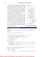
9.1 shows a lag-five simple moving average (SMA). The values are shown in the column
“Series value,” with the value of the average in the column “SMA5.” Each moving average
value is the average of the two series values above it, the one series value opposite and

the two next series values, making five series values in all. The column “SMA5 range”
shows which positions are included in any particular moving average value.
One drawback with SMAs, especially for long period weightings, is that the average
cannot begin to be calculated until the number of periods in the weighting has passed.
Also, the average value refers to the data point that is at the center of the weighting
period. (Table 9.1 plots the average of positions 1–5 in position 3.) With a weighting
period of, say, five days, the average can only be known as of two days ago. To know the
moving average value for today, two days have to pass.
Another potential drawback is that the contribution of each data point is equal to that of all
the other data points in the weighting period. It may be that the more distant past data
values are less relevant than more recent ones. This leads to the creation of a weighted
moving average (WMA). In such a construction, the data values are weighted so that the
more recent ones contribute more to the average value than earlier ones. Weights are
chosen for each point in the weighting period such that they sum to 1.
Table 9.2 shows the weights for constructing the lag-five WMA that is shown in Table 9.3.
The “v–4 indicates that the series value four steps back is used, and the weight “0.066”
indicates that the value with that lag is multiplied by the number 0.066, which is the
weight. The lag-five WMA’s value is calculated by multiplying the last five series values by
the appropriate weights.
TABLE 9.2 Weight for calculating a lag-five WMA.

Log

Weight

V-4

0.576766

V-3

0.423234

V-2

0.576766

V-1

0.423234

V0

0.576766

Please purchase PDF Split-Merge on www.verypdf.com to remove this watermark.


Wt total

1.000

TABLE 9.3 Log-five WMA

Position

Series value

WMA5

1

0.1338

2

0.4622

3

0.1448

4

0.6538

0.2966

5

0.0752

0.2833

6

0.2482

0.3161

7

0.4114

0.3331

8

0.3598

0.4796

9

0.7809

0.5303

10

0.5362

Table 9.3 shows the actual average values. Because of the weights, it is difficult to
“center” a WMA. Here it is shown “centered” one advanced on the lag-five SMA. This is
done because the weights favor the most recent values over the past values—so it should
be plotted to reflect that weighting.
Exponential moving averages (EMAs) solve the delay problem. Such averages consist of
two parts, a “head” and a “tail.” The tail value is the previous average value. The head

Please purchase PDF Split-Merge on www.verypdf.com to remove this watermark.

value is the current data value. The average’s value is found by moving the tail some way
closer to the head, but not all of the way. A weight is applied to decide how far to move the
tail toward the head. With light tail weights, the tail follows the head quite closely, and the
average behaves much like a short weighting period simple moving average. With heavier
tail weights, the tail moves more slowly, and it behaves somewhat like a longer-period
SMA. The head weight and the tail weight taken together must always sum to a value of 1.
No two averages behave in exactly the same way, but for EMAs, obviously the heavier
the head weight, the “faster” the EMA value will move—that is to say, the more closely it
follows the value of the series. For comparison, the EMA weights shown in Table 9.4
approximate the lag-five SMA.
TABLE 9.4 Head and tail weights to approximate a lag-five SMA.

Head weight

0.576766

Head weight

0.423234

Table 9.5 shows the actual values for the EMA. In this table, position 1 of the EMA is set
to the starting value of the series. The formula for determining the present value of the
EMA is
vEMA0 = (vs0 x wh) + (vEMA – 1 x wt)
where
vEMA0

is the value of the current EMA

vs0

is the current series value

wh

is the head weight

vEMA-1

is the last value of the EMA

wt

is the tail weight

TABLE 9.5 Values of the EMA

Please purchase PDF Split-Merge on www.verypdf.com to remove this watermark.


Position Series value

EMA

Head

Tail

1

0.1338

0.1338

2

0.4622

0.3232

0.2666

0.0566

3

0.1448

0.2203

0.0835

0.1956

4

0.6538

0.4703

0.3771

0.0613

5

0.0752

0.2424

0.0434

0.2767

6

0.2482

0.2458

0.1432

0.0318

7

0.4114

0.3413

0.2373

0.1051

8

0.3598

0.3519

0.2075

0.1741

9

0.7809

0.5993

0.4504

0.1523

10

0.5362

0.5629

0.3092

0.3305

This formula, with these weights, specifies that the current average value is found by
multiplying the current series value by 0.576766, and the last value of the average by
0.423243. The results are added together. The table shows the value of the series, the
current EMA, and the head and the tail values.
Figure 9.16 illustrates the moving averages discussed so far, and the effects of changing
the way they are constructed. The series itself changes value quite abruptly, and all of the
averages change more slowly. The SMA is the slowest to change of the averages shown.
The WMA moves similarly to the SMA, but clearly responds more to the recent values,
exactly as it is constructed to do.

Please purchase PDF Split-Merge on www.verypdf.com to remove this watermark.


Figure 9.16 Various moving averages and the effects of changing weights
showing SMAs, WMAs (weights shown separately), and EMAs (weights included
in formula). The graph illustrates the data shown in Tables 9.1, 9.2, and 9.5.

The EMA is the most responsive to the actual series value of the three averages shown.
Yet the weights were chosen to make it approximate the lag-five SMA average. Since
they seem to behave so differently, in what sense are these two approximately the same?
Over a longer series, with this set of weights, the EMA tends to be centered about the
value of the lag-five SMA. A series length of 10, as in the examples, is not sufficient to
show the effect clearly.
In general, as the lag periods get longer for SMAs and WMAs, or the head weights get

lighter (so the tail weights get heavier) for the EMAs, the average reacts more slowly to
changes in the series. Slow changes correspond to longer wavelengths, and longer
wavelengths are the same as lower frequencies. It is this ability to effectively change the
frequency at which the moving average reacts that makes them so useful as filters.
Although specific moving averages are constructed for specific purposes, for the
examples that follow later in the chapter, an EMA is the most convenient. The
convenience here is that given a data value (head), the immediate EMA past value (tail),
and the head and tail weights, then the EMA needs no delay before its value is known. It
is also quick and easy to calculate.
Moving averages can be used to separate series data into two frequency
domains—above and below the threshold set by the reactive frequency of the moving
average. How does this work in practice?

Moving Averages as Filters—Removing Noise
The composite-plus-noise waveform, first shown in Figure 9.7, seems to have a slower

Please purchase PDF Split-Merge on www.verypdf.com to remove this watermark.


cycle buried in higher-frequency noise. That is, buried in the rapid fluctuations, there
appears to be some slower fluctuation. Since this is a waveform built especially for the
example, this is in fact the case. However, nonmanufactured signals often show this type
of noise pattern too. Discovery of the underlying signal starts by trying to remove some of
the noise. Using an EMA, the high frequencies can be separated from the lower
frequencies.
High frequencies imply an EMA that moves fast. The speed of reaction of an EMA is set
by adjusting its weights. In this case, the head weight is set at 0.44 so that it moves very
fast. However, because of the tail weight, it cannot follow the fastest changes in the
waveform—and the fastest changes are the highest frequencies. The path of the EMA
itself represents the waveform without the higher frequencies. To separate out just the

high frequencies, subtract the EMA from the original waveform. The difference is the highfrequency component missing from the EMA trace. Figure 9.17 shows the original
waveform, waveform plus noise, EMA, and high frequencies remaining after subtraction.
Using an EMA with a head weight of 0.44 better resembles the original signal than the
noisy version because it has filtered out the high frequencies. Subtracting the EMA from
the noisy signal leaves the high frequencies removed by the EMA (top).

Figure 9.17 The original waveform, waveform plus noise, EMA, and high
frequencies remaining after subtraction.

It turns out that with this amount of weighting, the EMA is approximately equivalent to a
three-sample SMA (SMA3). An SMA3 has its value centered over position two, the middle
position. Doing this for the EMA used in the example recovers the original composite
waveform with a correlation of about 0.8127, as compared to the correlation for the signal
plus noise of about 0.6.

9.6.3 Smoothing 1—PVM Smoothing
There are many other methods for removing noise from an underlying waveform that do

Please purchase PDF Split-Merge on www.verypdf.com to remove this watermark.


not use moving averages as such. One of these is peak-valley-mean (PVM) smoothing.
Using PVM, a peak is defined as a value higher than the previous and next values. A
valley is defined as a value lower than the previous and next values. PVM smoothing uses
the mean of the last peak and valley (i.e., (P + V)/2) as the estimate of the underlying
waveform, instead of a moving average. The PVM retains the value of the last peak as the
current peak value until a new peak is discovered, and the same is true for the valleys.
This is the shortest possible PVM and covers three data points, so it is a lag-three PVM. It
should be noted that PVMs with other, larger lags are possible.
Figure 9.18 shows in the upper image the peak, valley, and mean values. The lower

image superimposes the recovered waveform on the original complex waveform without
any noise added. Once again, as with moving averages, the recovered waveform needs
to be centered appropriately. Centering again is at position two of three, halfway along the
lag distance, as from there it is always the last and next positions that are being
evaluated. The recovery is quite good, a correlation a little better than 0.8145, very similar
to the EMA method.

Figure 9.18 PVM smoothing: the peak, valley, and mean values for the
composite-plus-noise waveform (top) and the mean estimate superimposed on
the actual composite waveform (bottom).

9.6.4 Smoothing 2—Median Smoothing, Resmoothing, and
Hanning
Median smoothing uses “windows.” A window is a group of some specific number of
contiguous data points. It corresponds to the lag distance mentioned before. The only
difference between a window and a lag is that the data in a window is manipulated in
some way, say, changed in order. A lag implies that the data is not manipulated. As the
window moves through the series, the oldest data point is discarded, and a new one is

Please purchase PDF Split-Merge on www.verypdf.com to remove this watermark.


added. When median smoothing, use the median of the values in the window in place of
the actual value. A median is the value that comes in the middle of a list of values ordered
by value. When the window is an even length, use as the median value the average of the
two middle values in the list. In many ways, median smoothing is similar to average
smoothing except that the median is used instead of the average. Using the median
makes the smoothed value less sensitive to extremes in the window since it is always the
middle value of the ordered values that is taken. A single extreme value will never appear
in the middle of the ordered list, and thus does not affect the median value.

Resmoothing is a technique of smoothing the smoothed values. One form of resmoothing
continues until there is no change in the resmoothed waveform. Other resmoothing
techniques use a fixed number of resmooths, but vary the window size from smoothing to
smoothing.
Hanning is a technique borrowed from computer vision, where it is used for image
smoothing. Essentially it is a form of weighted averaging. The window is three long, left in
the original order, so it is really a lag. The three data points are multiplied by the weights
0.25, 0.50, 0.25, respectively. The hanning operation removes any final spikes left after
smoothing or resmoothing.
There are very many types of resmoothing. A couple of examples of the technique will be
briefly examined. The first, called “3R2H,” is a median smooth with a window of three,
repeated (the “R” in the name) until no change in the waveform occurs; then a median
smoothing with a window length of two; then one hanning operation. When applied to the
example waveform, this smoothing has a correlation with the original waveform of about
0.8082.
Another, called “4253H” smoothing, has four median smoothing operations with windows
of four, two, five, and three, respectively, followed by a hanning operation. This has a
correlation with the original example waveform of about 0.8030. Although not illustrated,
both of these smooths produce a waveform that appears to be very similar to that shown
in the lower image of Figure 9.18.
Again, although not illustrated, these techniques can be combined in almost any number
of ways. Smoothing the PVM waveform and performing the hanning operation, for
example, improves the fit with the original slightly to a correlation of about 0.8602.

9.6.5 Extraction
All of these methods remove noise or high-frequency components. Sometimes the
high-frequency components are not actually noise, but an integral part of the
measurement. If the miner is interested in the slower interactions, the high-frequency
component only serves to mask the slower interactions. Extracting the slower interactions
can be done in several ways, including moving averages and smoothing. The various

Please purchase PDF Split-Merge on www.verypdf.com to remove this watermark.


smoothing and filtering operations can be combined in numerous ways, just as smoothing
and hanning the PVM smooth shows. Many other filtering methods are also available,
some based on very sophisticated mathematics. All are intended to separate information
in the waveform into its component parts.
What is extracted by the techniques described here comes in two parts, high and lower
frequencies. The first part is the filtered or smoothed part. The remainder forms the
second part and is found by subtracting the first part, the filtered waveform, from the
original waveform. When further extraction is made on either, or both, of the extracted
waveforms, this is called reextraction. There seems to be an endless array of smoothing
and resmoothing, extraction and reextraction possibilities!
Waveforms can be separated in high-, middle-, and low-frequency components—and
then the separated components further separated. Here is where the miner must use
judgment. Examination of the extracted waveforms is called for—indeed, it is essential.
The object of all filtering and smoothing is to separate waveforms with pattern from noise.
The time to stop is when the extraction provides no additional separation. But how does
the miner know when to stop?
This is where the spectra and correlograms are very useful. The noise spectrum (Figure
9.7) and correlogram (Figure 9.11) show that noise, at least of the sort shown here, has a
fairly uniform spectrum and uniformly low autocorrelation at all lags. There still might be
useful information contained in the waveform, but the chance is small. This is a good sign
that extra effort will probably be better placed elsewhere. But what of the random walk?
Here there is a strong correlation in the correlogram, and the spectrum shows clear
peaks. Is there any way to determine that this is random walking?

9.6.6 Differencing
Differencing a waveform provides another powerful way to look at the information it

contains. The method takes the difference between each value and some previous value,
and analyzes the differences. A lag value determines exactly which previous value is
used, the lag having the same meaning as mentioned previously. A lag of one, for
instance, takes the difference between a value and the immediately preceding value.
The actual differences tend to appear noisy, and it is often very hard to see any pattern
when the difference values are plotted. Figure 9.19 shows the lag-one difference plot for
the composite-plus-noise waveform (left). It is hard to see what, if anything, this plot
indicates about the regularity and predictability of the waveform! Figure 9.19 also shows
the lag-one difference plot for the complex waveform without noise added (right). Here it is
easy to see that the differences are regular, but that was easy to see from the waveform
itself too—little is learned from the regularity shown.

Please purchase PDF Split-Merge on www.verypdf.com to remove this watermark.


Figure 9.19 Log-one difference plots: composite-plus-noise waveform
differences (left) and pattern of differences for the composite waveform without
noise (right).

Forward Differencing
Looking at the spectra and correlograms of the lag-one difference plots, however, does
reveal information. When first seen, the spectra and correlograms shown in Figure 9.20
look somewhat surprising. It is worth looking back to compare them with the
nondifferenced spectra for the same waveforms in Figures 9.6, 9.7, and 9.9, and the
nondifferenced correlograms in Figure 9.11.

Figure 9.20 Differences spectra and correlograms for various waveforms.

Figure 9.20(a) shows that the differenced composite waveform contains little spectral
energy at any of the frequencies shown. What energy exists is in the lower frequencies as

before. The correlogram for the same waveform still shows a high correlation, as
expected.
In Figure 9.20(b), the noise waveform, the differencing makes a remarkable difference to
the power spectrum. High energy at high frequencies—but the correlogram shows little

Please purchase PDF Split-Merge on www.verypdf.com to remove this watermark.


correlation at any lag.
Although the differenced noise spectrum in Figure 9.20(b) is remarkably changed, it is
nothing like the spectrum for the differenced random walk in 9.20(d). Yet both of these
waveforms were created from random noise. What is actually going on here?

Randomness Detector?
What is happening that makes the random waveforms produce such different spectra?
The noise power spectrum (shown in Figure 9.7) is fairly flat. Differencing it, as shown in
Figure 9.20(b), amplified—made larger—the higher frequencies. In fact, the higher the
frequency, the more the amplification. At the same time, differencing attenuated—made
smaller—the lower frequencies. So differencing serves as a high-pass filter.
What of the random walk? The random walk was actually constructed by taking random
noise, in the form of numbers in the range of –1 to +1, and adding them together step by
step. When this was differenced, back came the original random noise used to generate
it. In other words, creating a walk, or “undifferencing,” serves to amplify the low
frequencies and attenuate the high frequencies—exactly the opposite of differencing!
Building the random walk obviously did something that hid the underlying nature of the
random noise used to construct it. When differenced, the building process was undone,
and back came a spectrum characteristic of noise. So, to go back to the question, “Is
there a way to tell that the random walk is generated by a random process?” the answer is
a definite “maybe.” Differencing can at least give some clues that the waveform was
generated by some process that, at least by this test, looks random.

There is no way to tell from the series itself if the random walk is in fact random. That
requires knowing the underlying process in the real world that is actually responsible for
producing the series. The numbers used here, for instance, were not actually random, but
what is known as pseudo-random. (Genuinely random numbers turn out to be fiendishly
difficult to come by!) A computer algorithm was used that has an internal mechanism that
produces a string of numbers that pass certain tests for randomness. However, the
sequence is actually precisely defined, and not random at all. Nonetheless, it looks
random, and lacking an underlying explanation, which may or may not be predictive, it is
at least known to have some of the properties of a random number. Simply finding a
spectrum indicating possible randomness only serves as a flag that more tests are
needed. If it eventually passes enough tests, this indeed serves as a practical definition of
randomness. What constitutes “enough” tests depends on the miner and the needs of the
application. But nonetheless, the working definition of randomness for a series is simply
one that passes all the tests of randomness and has no underlying explanation that shows
it to be otherwise.

Reverse Differencing (Summing)

Please purchase PDF Split-Merge on www.verypdf.com to remove this watermark.


Interestingly, discovering a way to potentially expose random characteristics used the
reverse process of differencing. Building the random walk required adding together
random distance and direction steps generated by random noise. It turns out that creating
any series in a similar way is the equivalent of reverse differencing! (This, of course, is
summing—the exact opposite of taking a difference. “Reverse differencing” seems more
descriptive.) Without going into details, the power spectrum and correlogram for the
reverse-differenced composite-plus-noise waveform is shown in Figure 9.21. The power
spectrum shows the low-frequency amplification, high-frequency attenuation that is the
opposite effect of forward differencing. The correlogram is interesting as the correlation

curve is much stronger altogether when the high-frequency components are attenuated.
In this case, the reverse-differenced curve becomes very highly autocorrelated—in other
words, highly predictable.

Figure 9.21 Effects of reverse differencing. Low frequencies are enhanced, and
high frequencies are attenuated.

Just as differencing can yield insights, so too can summing. Linearly detrending the
waveform before the summing operation may help too.

9.7 Other Problems
So far, the problems examined have been specific to series data. The solutions have
focused on ways of extracting information from noisy or distorted series data. They have
involved extracting a variety of waveforms from the original waveform that emphasize
particular aspects of the data useful for modeling. But whatever has been pulled out, or
extracted, from the original series, it is still in the form of another series. It is quite possible
to look at the distribution of values in such a series exactly as if it were not a series. That
is to say, taking care not to actually lose the indexing, the variable can be treated exactly
as if it were a nonseries variable. Looking at the series this way allows some of the tools

Please purchase PDF Split-Merge on www.verypdf.com to remove this watermark.


used for nonseries data to be applied to series data. Can this be done, and where does it
help?

9.7.1 Numerating Alpha Values
As mentioned in the introduction to this chapter, numeration of alpha values in a series
presents some difficulties. It can be done, but alpha series values are almost never found
in practice. On the rare occasions when they do occur, numerating them using the

nonseries techniques already discussed, while not providing an optimal numeration, does
far better than numeration without any rationale. Random or arbitrary assignment of
values to alpha labels is always damaging, and is just as damaging when the data is a
series. It is not optimal because the ordering information is not fully used in the
numeration. However, using such information involves projecting the alpha values in a
nonlinear phase space that is difficult to discover and computationally intense to
manipulate. Establishing the nonlinear modes presents problems because they too have
to be constructed from the components cycle, season, trend, and noise. Accurately
determining those components is not straightforward, as we have seen in this chapter.
This enormously compounds the problem of in-series numeration.
The good news is that, with time series in particular, it seems easier to find an appropriate
rationale for numerating alpha values from a domain expert than for nonseries data.
Reverse pivoting the alphas into a table format, and numerating them there, is a good
approach. However, the caveat has to be noted that since alpha numerated series occur
so rarely, there is little experience to draw on when preparing them for mining. This makes
it difficult to draw any hard and fast general conclusions.

9.7.2 Distribution
As far as distributions are concerned, a series variable has a distribution that exists
without reference to the ordering. When looked at in this way, so long as the
ordering—that is, the index variable—is not disturbed, the displacement variable can be
redistributed in exactly the same manner as a nonseries variable. Chapter 7 discussed
the nature of distributions, and reasons and methods for redistributing values. The
rationale and methods of redistribution are similar for series data and may be even more
applicable in some ways. There are time series methods that require the variables’ data to
be centered (equally distributed above and below the mean) and normalized. For series
data, the distribution should be normalized after removing any trend.
When modeling series data, the series should, if possible, be what is known as stationary.
A stationary series has no trend and constant variance over the length of the series, so it
fluctuates uniformly about a constant level.

Redistribution Modifying Waveform Shape

Please purchase PDF Split-Merge on www.verypdf.com to remove this watermark.


Redistribution as described in Chapter 7, when applied to series variables’ data, goes far
toward achieving a stationary series. Any series variable can be redistributed exactly as
described for nonseries. However, this is not always an unambiguous blessing! (More
dragons.) Whenever the distribution of a variable is altered, the transform required is
captured so that it can always be undone. Indeed, the PIE-O has to undo any
transformation for any output variables. However, it may be that the exact shape of the
waveform is important to the modeling tool. (Only the modeler is in a position to know for
sure if this is the case at modeling time.) If so, the redistribution may introduce unwanted
distortion. In Figure 9.22, the top-left image shows a histogram of the distribution of values
for the sine wave. Redistribution creates a rectangular distribution, shown in the top-right
image. But redistribution changes the nature of the shape of the wave! The lower image
shows both a sine wave and the wave shape after redistribution. Redistribution is
intended to do exactly what is seen here—all of the nonlinearity has been removed. The
curved waveform is translated into a linear representation—thus the straight lines. This
may or may not cause a problem. However, the miner must be aware of the issue.

Figure 9.22 Redistributing the distribution linearizes the nonlinear waveform. As
the distribution of a pure sine wave is adjusted to be nearer rectangular, so the
curves are straightened. If maintaining the wave shape is important, some other
transform is required.

Distribution Maintaining Waveform Shape
Redistribution goes a long way toward equalizing the variance. However, some other
method is required if the wave shape needs to be retained. If the variance of the series

changes as the series progresses, it may be possible to transform the values so that the
variance is more constant. Erratic fluctuations of variance over the length of the series
cause more problems, but may be helped by a transformation. A “Box-Cox”
transformation (named after the people who first described it) may work well. The

Please purchase PDF Split-Merge on www.verypdf.com to remove this watermark.


transform is fairly simple to apply, and is as follows:

When the changing variance is adjusted, the distribution still has to be balanced. A
second transform accomplishes this. The second transform subtracts the mean of the
transformed variable from each transformed value, and divides the result by the standard
deviation. The formula for this second transformation is

The index, or displacement, variable should not be redistributed, even if it is of unequal
increments.

9.7.3 Normalization
Normalization over the range of 0 to 1 needs no modification. The displacement variable can
be normalized using exactly the same techniques (described in Chapter 7) that work for
nonseries data.

9.7 Other Problems
So far, the problems examined have been specific to series data. The solutions have
focused on ways of extracting information from noisy or distorted series data. They have
involved extracting a variety of waveforms from the original waveform that emphasize
particular aspects of the data useful for modeling. But whatever has been pulled out, or
extracted, from the original series, it is still in the form of another series. It is quite possible
to look at the distribution of values in such a series exactly as if it were not a series. That

is to say, taking care not to actually lose the indexing, the variable can be treated exactly
as if it were a nonseries variable. Looking at the series this way allows some of the tools
used for nonseries data to be applied to series data. Can this be done, and where does it
help?

9.7.1 Numerating Alpha Values

Please purchase PDF Split-Merge on www.verypdf.com to remove this watermark.


As mentioned in the introduction to this chapter, numeration of alpha values in a series
presents some difficulties. It can be done, but alpha series values are almost never found
in practice. On the rare occasions when they do occur, numerating them using the
nonseries techniques already discussed, while not providing an optimal numeration, does
far better than numeration without any rationale. Random or arbitrary assignment of
values to alpha labels is always damaging, and is just as damaging when the data is a
series. It is not optimal because the ordering information is not fully used in the
numeration. However, using such information involves projecting the alpha values in a
nonlinear phase space that is difficult to discover and computationally intense to
manipulate. Establishing the nonlinear modes presents problems because they too have
to be constructed from the components cycle, season, trend, and noise. Accurately
determining those components is not straightforward, as we have seen in this chapter.
This enormously compounds the problem of in-series numeration.
The good news is that, with time series in particular, it seems easier to find an appropriate
rationale for numerating alpha values from a domain expert than for nonseries data.
Reverse pivoting the alphas into a table format, and numerating them there, is a good
approach. However, the caveat has to be noted that since alpha numerated series occur
so rarely, there is little experience to draw on when preparing them for mining. This makes
it difficult to draw any hard and fast general conclusions.

9.7.2 Distribution
As far as distributions are concerned, a series variable has a distribution that exists
without reference to the ordering. When looked at in this way, so long as the
ordering—that is, the index variable—is not disturbed, the displacement variable can be
redistributed in exactly the same manner as a nonseries variable. Chapter 7 discussed
the nature of distributions, and reasons and methods for redistributing values. The
rationale and methods of redistribution are similar for series data and may be even more
applicable in some ways. There are time series methods that require the variables’ data to
be centered (equally distributed above and below the mean) and normalized. For series
data, the distribution should be normalized after removing any trend.
When modeling series data, the series should, if possible, be what is known as stationary.
A stationary series has no trend and constant variance over the length of the series, so it
fluctuates uniformly about a constant level.

Redistribution Modifying Waveform Shape
Redistribution as described in Chapter 7, when applied to series variables’ data, goes far
toward achieving a stationary series. Any series variable can be redistributed exactly as
described for nonseries. However, this is not always an unambiguous blessing! (More
dragons.) Whenever the distribution of a variable is altered, the transform required is

Please purchase PDF Split-Merge on www.verypdf.com to remove this watermark.


captured so that it can always be undone. Indeed, the PIE-O has to undo any
transformation for any output variables. However, it may be that the exact shape of the
waveform is important to the modeling tool. (Only the modeler is in a position to know for
sure if this is the case at modeling time.) If so, the redistribution may introduce unwanted
distortion. In Figure 9.22, the top-left image shows a histogram of the distribution of values
for the sine wave. Redistribution creates a rectangular distribution, shown in the top-right
image. But redistribution changes the nature of the shape of the wave! The lower image

shows both a sine wave and the wave shape after redistribution. Redistribution is
intended to do exactly what is seen here—all of the nonlinearity has been removed. The
curved waveform is translated into a linear representation—thus the straight lines. This
may or may not cause a problem. However, the miner must be aware of the issue.

Figure 9.22 Redistributing the distribution linearizes the nonlinear waveform. As
the distribution of a pure sine wave is adjusted to be nearer rectangular, so the
curves are straightened. If maintaining the wave shape is important, some other
transform is required.

Distribution Maintaining Waveform Shape
Redistribution goes a long way toward equalizing the variance. However, some other
method is required if the wave shape needs to be retained. If the variance of the series
changes as the series progresses, it may be possible to transform the values so that the
variance is more constant. Erratic fluctuations of variance over the length of the series
cause more problems, but may be helped by a transformation. A “Box-Cox”
transformation (named after the people who first described it) may work well. The
transform is fairly simple to apply, and is as follows:

Please purchase PDF Split-Merge on www.verypdf.com to remove this watermark.


When the changing variance is adjusted, the distribution still has to be balanced. A
second transform accomplishes this. The second transform subtracts the mean of the
transformed variable from each transformed value, and divides the result by the standard
deviation. The formula for this second transformation is

The index, or displacement, variable should not be redistributed, even if it is of unequal
increments.

9.7.3 Normalization
Normalization over the range of 0 to 1 needs no modification. The displacement variable can
be normalized using exactly the same techniques (described in Chapter 7) that work for
nonseries data.

9.8 Preparing Series Data
A lot of ground was covered in this chapter. A brief review will help before pulling all the
pieces together and looking at a process for actually preparing series data.
• Series come in various types, of which the most common by far is the time series. All
series share a common structure in that the ordering of the measurements carries
information that the miner needs to use.
• Series data can be completely described in terms of its four component parts: trend,
cycles, seasonality, and noise. Alternatively, series can also be completely described as
consisting of sine and cosine waveforms in various numbers and of various amplitudes,
phases, and frequencies. Tools to discover the various components include Fourier
analysis, power spectra, and correlograms.
• Series data are modeled either to discover the effects of time or to look at how the data

Please purchase PDF Split-Merge on www.verypdf.com to remove this watermark.


changes in time.
• Series data shares all the problems that nonseries data has, plus several that are
unique to series.
— Missing values require special procedures, and care needs to be taken not to insert a
pattern into the missing values by replicating part of a pattern found elsewhere in the
series.
— Nonuniform displacement is dealt with as if it were any other form of noise.
— Trend needs special handling, exactly as any other monotonic value.
• Various techniques exist for filtering out components of the total waveform. They

include, as well as complex mathematical devices for filtering frequencies,
— Moving averages of various types. A moving average involves using lagged values
over the series data points and using all of the lagged values in some way to
reestimate the data point value. A large variety of moving average techniques exist,
including simple moving averages (SMAs), weighted moving averages (WMAs), and
exponential moving averages (EMAs).
— Smoothing techniques of several types. Smoothing is a windowing technique in
which a window of adjustable length selects a particular subseries of data points for
manipulation. The window slides over the whole series and manipulates each
separate subset of data points to reestimate the window’s central data point value.
Smoothing techniques include peak-valley-mean (PVM), median smoothing, and
Hanning.
— Resmoothing is a smoothing technique that involves either reapplying the same
smoothing technique several times until no change occurs, or applying different
window sizes or techniques several times.
• Differencing and reverse differencing (summing) offer alternative ways of looking at
high- or low-frequency components of a waveform. Differencing and summing also
transform waveforms in ways that may give clues to underlying randomness.
• The series data alone cannot ever be positively determined to contain a random
component, although additional tests can raise the confidence level that detected noise
is randomly generated. Only a rationale or causal explanation external to the data can
confirm random noise generation.
• Components of a waveform can be separated out from the original waveform using one
or several of the above techniques. These components are themselves series that

Please purchase PDF Split-Merge on www.verypdf.com to remove this watermark.


express some part of the information contained in the whole original series. Having the
parts separated aids modeling by making the model either more understandable or

more predictive, or meets some other need of the miner.

9.8.1 Looking at the Data
Series data must be looked at. There is positively no substitute whatsoever for looking at
the data—graphing it, looking at correlograms, looking at spectra, differencing, and so on.
There are a huge variety of other powerful tools used for analyzing series data, but those
mentioned here, at least, must be used to prepare series data. The best aid that the miner
has is a powerful series data manipulation and visualization tool, and preferably one that
allows on-the-fly data manipulation, as well as use of the tools discussed. The underlying
software used here to manipulate data and produce the images used for illustration was
Statistica. (The accompanying CD-ROM includes a demonstration version.) This is one of
several powerful statistical software packages that easily and quickly perform these and
many other manipulations. Looking at the information revealed, and becoming familiar
with what it means, is without any doubt the miner’s most important tool in preparing
series data. It is, after all, the only way to look for dragons, chimera, and quicksand, not to
mention the marked rocky road!

9.8.2 Signposts on the Rocky Road
So how should the miner use these tools and pointers when faced with series data? Here
is a possible plan of attack.
• Plot the data Not only at the beginning should the data be plotted—plot everything.
Keep plotting. Plot noise, plot smoothed, look at correlograms, look at spectra—and
keep doing it. Work with it. Get a feel for what is in the data. Simply play with it. Video
games with series data! This is not a frivolous approach. There is no more powerful
pattern recognition tool known than the one inside the human head. Look and think
closely about what is in the data and what it might mean. Although stated first, this is a
continuous activity for all the stages that follow.
• Fill in missing values After a first look at the data, decide what to do about any that is
missing. If possible, find any missing values. Seek them out. Digging them up, if at all
possible, is a far better alternative than making them up! If they positively are not

available, build autoregressive models and replace them.
Now—build models before and after replacement! The “before” models will use subsets of
the data without any missing values. Build “after” models of the same sample length as
the “before” models, but include the replaced values. If possible, build several “after”
models with the replaced values at the beginning, middle, and end of the series. At least
build “after” models with the replaced values at different places in the modeled series.

Please purchase PDF Split-Merge on www.verypdf.com to remove this watermark.


What changes? What is the relative strength of the patterns “discovered” in the “after”
models that are not in the “before” models? If specific strong patterns only appear in the
“after” models, try diluting them by adding neutral white noise to the replaced values. Look
again. Try again. Keep trying until the replacement values appear to make no noticeable
difference to the pattern density.
• Replace outliers Are there outliers? Are they really outliers, or just extremes of the
range? Can individual outliers be accounted for as measurement error? Are there runs
of outliers? If so, what process could cause them? Can the values be translated into the
normal range?
Just as with missing values, work at finding out what caused the outliers and finding the
accurate values. If they are positively not available, replace them exactly as for missing
values.
• Remove trend Linear trend is easy to remove. Try fitting some other fractional frequency
trend lines if they look like they might fit. If uncertain, fit a few different trend lines—log,
square, exponential—see what they look like. Does one of them seem to fit some
underlying trend in the data? If so, subtract it from the data. When graphed, does the
data fit the horizontal axis better? If yes, fine. If no, keep trying.
• Adjust variance Subtract out the trend. Eyeball the variance, that is, the way the data
scatters along the horizontal axis. Is it constant? Does it increase or decrease as the
series progresses? If it isn’t constant, try Box-Cox transforms (or other transforms if they

feel more comfortable). Get the variance as uniform as possible.
• Smooth Try various smoothing techniques, if needed. Unless there is some good
reason to expect sharp spikes in the data, use hanning to get rid of them. Look at the
spectrum. Look at the correlogram. Does smoothing help make what is happening in the
data clearer? Subtract out the high frequencies and look at them. What is left in there?
Any pattern? Mainly random? Extract what is in the noise until what is left seems
random.
Now start again using forward and reverse differencing. Same patterns found? If not, why
not? If so, why? Which makes most sense?
• Account for seasonalities Are there seasonal effects? What are they? Can they be
identified? Subtract them out. If possible, create a separate variable for each, or a
separate alpha label if more appropriate (so that when building a model, the model
“knows” about the seasonalities).
• Extract main cycle Look for the main underlying “heartbeat” in the data. Smooth and
filter until it seems clear. Extract it from the data.

Please purchase PDF Split-Merge on www.verypdf.com to remove this watermark.


• Extract minor cycles Look at what is left in the “noise.” Smooth it again. PVM works well
very often. Look at spectra and correlograms. Any pattern? If so, extract it.
Look at the main waveform—the heartbeat. Look with a spectrum. What are the main
component frequencies? Does this make sense? Is it reasonable to expect this set of
frequencies? If it cannot be explained, is there at least no reason that it shouldn’t be so?
• Redistribute and normalize Redistribute and normalize the values if strictly maintaining
the waveform shape is not critical; otherwise, just normalize.
• Model or reverse pivot If modeling the series, time to start. Otherwise, reverse pivot. For
the reverse pivot, build an array of variables of different lags that are least correlated with
each other. Try a variable for each of the main frequencies. Try a variable for the main
cycle. Try a variable for the noise level. Survey the results. (When modeling, build several

quick models to see which looks like it might work best.)

9.9 Implementation Notes
Familiarity with what displacement series look like and hands-on experience are the best
data preparation tool that a miner can find for preparing series data. As computer systems
become ever more powerful, it appears that there are various heuristic and algorithmic
procedures that will allow automated series data preparation. Testing the performance of
these procedures awaits the arrival of yet more powerful, low-cost computer systems.
This has already happened with nonseries data preparation algorithms as the
demonstration code shows. What is here today is a stunning array of automated tools for
letting the miner look at series data in a phenomenal number of ways. This chapter hardly
scratched the surface of the full panoply of techniques available. The tools that are
available put power to look into the miners’ hands that has never before been available.
The ability to see has to be found by experience.
Since handling series data is a very highly visual activity, and since fully automated
preparation is so potentially damaging to data, the demonstration software has no specific
routines for preparing displacement series data. Data visualization is a broad field in itself,
and there are many highly powerful tools for handling data that have superb visualization
capability. For small to moderate data sets, even a spreadsheet can serve as a good
place to start. Spectral analysis is difficult, although not impossible, and correlograms are
fairly easy. Moving on from there are many other reasonably priced data imaging and
manipulation tools. Data imaging is so broad and deep a field, it is impossible to begin to
cover the topic here.
This chapter has dealt exclusively with displacement series data. The miner has covered
sufficient ground to prepare the series data so that it can be modeled. Having prepared such
data, it can be modeled using the full array of the miner’s tools. As with previous chapters,
attention is now turned back to looking at data without considering the information contained

Please purchase PDF Split-Merge on www.verypdf.com to remove this watermark.

in any ordering. It is time to examine the data set as a whole.

Please purchase PDF Split-Merge on www.verypdf.com to remove this watermark.