Tài liệu Evaluation of Functions part 10 pptx

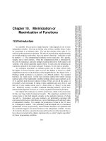
5.9 Derivatives or Integrals of a Chebyshev-approximated Function
195
Sample page from NUMERICAL RECIPES IN C: THE ART OF SCIENTIFIC COMPUTING (ISBN 0-521-43108-5)
Copyright (C) 1988-1992 by Cambridge University Press.Programs Copyright (C) 1988-1992 by Numerical Recipes Software.
Permission is granted for internet users to make one paper copy for their own personal use. Further reproduction, or any copying of machine-
readable files (including this one) to any servercomputer, is strictly prohibited. To order Numerical Recipes books,diskettes, or CDROMs
visit website or call 1-800-872-7423 (North America only),or send email to (outside North America).
5.9 Derivatives or Integrals of a
Chebyshev-approximated Function
If you have obtained the Chebyshev coefficients that approximate a function in
a certain range (e.g., from chebft in §5.8), then it is a simple matter to transform
them to Chebyshev coefficients corresponding to the derivative or integral of the
function. Having done this, you can evaluate the derivative or integral just as if it
were a function that you had Chebyshev-fitted ab initio.
The relevant formulas are these: If c
i
,i=0,...,m−1 are the coefficients
that approximate a function f in equation (5.8.9), C
i
are the coefficients that
approximate the indefinite integral of f,and c

i
are the coefficients that approximate
the derivative of f,then
C
i
=
c
i−1
−c

i+1
2(i − 1)
(i>1) (5.9.1)
c

i−1
= c

i+1
+2(i−1)c
i
(i = m − 1,m−2,...,2) (5.9.2)
Equation (5.9.1) is augmented by an arbitrary choice of C
0
, corresponding to an
arbitrary constant of integration. Equation (5.9.2), which is a recurrence, is started
with the values c

m
= c

m−1
=0, corresponding to no information about the m +1st
Chebyshev coefficient of the original function f.
Here are routines for implementing equations (5.9.1) and (5.9.2).
void chder(float a, float b, float c[], float cder[], int n)
Given
a,b,c[0..n-1]
, as output from routine
chebft

§5.8,andgiven
n
, the desired degree
of approximation (length of
c
to be used), this routine returns the array
cder[0..n-1]
,the
Chebyshev coefficients of the derivative of the function whose coefficients are
c
.
{
int j;
float con;
cder[n-1]=0.0; n-1 and n-2 are special cases.
cder[n-2]=2*(n-1)*c[n-1];
for (j=n-3;j>=0;j--)
cder[j]=cder[j+2]+2*(j+1)*c[j+1]; Equation (5.9.2).
con=2.0/(b-a);
for (j=0;j<n;j++) Normalize to the interval b-a.
cder[j] *= con;
}
void chint(float a, float b, float c[], float cint[], int n)
Given
a,b,c[0..n-1]
, as output from routine
chebft
§5.8,andgiven
n
, the desired degree

of approximation (length of
c
to be used), this routine returns the array
cint[0..n-1]
,the
Chebyshev coefficients of the integral of the function whose coefficients are
c
. The constant of
integration is set so that the integral vanishes at
a
.
{
int j;
float sum=0.0,fac=1.0,con;
con=0.25*(b-a); Factor that normalizes to the interval b-a.
for (j=1;j<=n-2;j++) {
cint[j]=con*(c[j-1]-c[j+1])/j; Equation (5.9.1).
196
Chapter 5. Evaluation of Functions
Sample page from NUMERICAL RECIPES IN C: THE ART OF SCIENTIFIC COMPUTING (ISBN 0-521-43108-5)
Copyright (C) 1988-1992 by Cambridge University Press.Programs Copyright (C) 1988-1992 by Numerical Recipes Software.
Permission is granted for internet users to make one paper copy for their own personal use. Further reproduction, or any copying of machine-
readable files (including this one) to any servercomputer, is strictly prohibited. To order Numerical Recipes books,diskettes, or CDROMs
visit website or call 1-800-872-7423 (North America only),or send email to (outside North America).
sum += fac*cint[j]; Accumulates the constant of integration.
fac = -fac; Will equal ±1.
}
cint[n-1]=con*c[n-2]/(n-1); Special case of (5.9.1) for n-1.
sum += fac*cint[n-1];
cint[0]=2.0*sum; Set the constant of integration.

}
Clenshaw-Curtis Quadrature
Since a smooth function’s Chebyshev coefficients c
i
decrease rapidly, generally expo-
nentially, equation (5.9.1) is often quite efficient as the basis for a quadrature scheme. The
routines chebft and chint, used in that order, can be followed by repeated calls to chebev
if

x
a
f (x)dx is required for many different values of x in the range a ≤ x ≤ b.
If only the single definite integral

b
a
f(x)dx is required, then chint and chebev are
replaced by the simpler formula, derived from equation (5.9.1),

b
a
f(x)dx =(b−a)

1
2
c
1
−
1
3

c
3
−
1
15
c
5
−···−
1
(2k + 1)(2k − 1)
c
2k+1
−···

(5.9.3)
where the c
i
’s are as returned by chebft. The series can be truncated when c
2k+1
becomes
negligible, and the first neglected term gives an error estimate.
This scheme is known as Clenshaw-Curtis quadrature
[1]
. It is often combined with an
adaptive choice of N, the number of Chebyshev coefficients calculated via equation (5.8.7),
which is also the number of function evaluations of f(x). If a modest choice of N does
not give a sufficiently small c
2k+1
in equation (5.9.3), then a larger value is tried. In this
adaptive case, it is even better to replace equation (5.8.7) by the so-called “trapezoidal” or

Gauss-Lobatto (§4.5) variant,
c
j
=
2
N
N


k=0
f

cos

πk
N

cos

π(j − 1)k
N

j =1,...,N (5.9.4)
where (N.B.!) the two primes signify that the first and last terms in the sum are to be
multiplied by 1/2.IfNis doubled in equation (5.9.4), then half of the new function
evaluation points are identical to the old ones, allowing the previous function evaluations to be
reused. This feature, plus the analytic weights and abscissas (cosine functions in 5.9.4), give
Clenshaw-Curtis quadrature an edge over high-order adaptive Gaussian quadrature (cf. §4.5),
which the method otherwise resembles.
If yourproblemforces youtolarge valuesof N, you shouldbe aware thatequation(5.9.4)

can be evaluated rapidly, and simultaneously for all the values of j, by a fast cosine transform.
(See §12.3, especially equation 12.3.17.) (We already remarked that the nontrapezoidal form
(5.8.7) can also be done by fast cosine methods, cf. equation 12.3.22.)
CITED REFERENCES AND FURTHER READING:
Goodwin, E.T. (ed.) 1961,
Modern Computing Methods
, 2nd ed. (New York: Philosophical Li-
brary), pp. 78–79.
Clenshaw, C.W., and Curtis, A.R. 1960,
Numerische Mathematik
, vol. 2, pp. 197–205. [1]
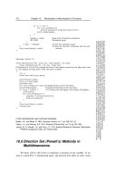
5.10 Polynomial Approximation from Chebyshev Coefficients
197
Sample page from NUMERICAL RECIPES IN C: THE ART OF SCIENTIFIC COMPUTING (ISBN 0-521-43108-5)
Copyright (C) 1988-1992 by Cambridge University Press.Programs Copyright (C) 1988-1992 by Numerical Recipes Software.
Permission is granted for internet users to make one paper copy for their own personal use. Further reproduction, or any copying of machine-
readable files (including this one) to any servercomputer, is strictly prohibited. To order Numerical Recipes books,diskettes, or CDROMs
visit website or call 1-800-872-7423 (North America only),or send email to (outside North America).
5.10 Polynomial Approximation from
Chebyshev Coefficients
You may well ask after reading the preceding two sections, “Must I store and
evaluate my Chebyshev approximation as an array of Chebyshev coefficients for a
transformed variable y? Can’t I convert the c
k
’s into actual polynomial coefficients
in the original variable x and have an approximation of the following form?”
f(x) ≈
m−1

k=0

g
k
x
k
(5.10.1)
Yes, you can do this (and we will give you the algorithm to do it), but we
caution you against it: Evaluating equation (5.10.1), where the coefficient g’s reflect
an underlying Chebyshev approximation, usually requires more significant figures
than evaluation of the Chebyshev sum directly (as by chebev). This is because
the Chebyshev polynomials themselves exhibit a rather delicate cancellation: The
leading coefficient of T
n
(x), for example, is 2
n−1
; other coefficients of T
n
(x) are
even bigger; yet they all manage to combine into a polynomial that lies between ±1.
Only when m is no larger than 7 or 8 should you contemplate writing a Chebyshev
fit as a direct polynomial, and even in those cases you should be willing to tolerate
two or so significant figures less accuracy than the roundoff limit of your machine.
You get the g’s in equation (5.10.1) from the c’s output from chebft (suitably
truncated at a modest value of m)bycallinginsequencethefollowingtwoprocedures:
#include "nrutil.h"
void chebpc(float c[], float d[], int n)
Chebyshev polynomial coefficients. Given a coefficient array
c[0..n-1]
, this routine generates
a coefficient array
d[0..n-1]

such that

n-1
k=0
d
k
y
k
=

n-1
k=0
c
k
T
k
(y) −
c
0
/2.Themethod
is Clenshaw’s recurrence (5.8.11), but now applied algebraically rather than arithmetically.
{
int k,j;
float sv,*dd;
dd=vector(0,n-1);
for (j=0;j<n;j++) d[j]=dd[j]=0.0;
d[0]=c[n-1];
for (j=n-2;j>=1;j--) {
for (k=n-j;k>=1;k--) {
sv=d[k];

d[k]=2.0*d[k-1]-dd[k];
dd[k]=sv;
}
sv=d[0];
d[0] = -dd[0]+c[j];
dd[0]=sv;
}
for (j=n-1;j>=1;j--)
d[j]=d[j-1]-dd[j];
d[0] = -dd[0]+0.5*c[0];
free_vector(dd,0,n-1);
}