Tài liệu RF và mạch lạc lò vi sóng P7 pptx

7
TWO-PORT NETWORKS
Electronic circuits are frequently needed for processing a given electrical signal to
extract the desired information or characteristics. This includes boosting the strength
of a weak signal or ®ltering out certain frequency bands and so forth. Most of these
circuits can be modeled as a black box that contains a linear network comprising
resistors, inductors, capacitors, and dependent sources. Thus, it may include
electronic devices but not the independent sources. Further, it has four terminals,
two for input and the other two for output of the signal. There may be a few more
terminals to supply the bias voltage for electronic devices. However, these bias
conditions are embedded in equivalent dependent sources. Hence, a large class of
electronic circuits can be modeled as two-port networks. Parameters of the two-port
completely describe its behavior in terms of voltage and current at each port. These
parameters simplify the description of its operation when the two-port network is
connected into a larger system.
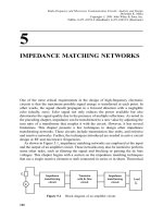
Figure 7.1 shows a two-port network along with appropriate voltages and currents
at its terminals. Sometimes, port-1 is called the input while port-2 is the output port.
The upper terminal is customarily assumed to be positive with respect to the lower
one on either side. Further, currents enter the positive terminals at each port. Since
243
Figure 7.1 Two-port network.
Radio-Frequency and Microwave Communication Circuits: Analysis and Design
Devendra K. Misra
Copyright # 2001 John Wiley & Sons, Inc.
ISBNs: 0-471-41253-8 (Hardback); 0-471-22435-9 (Electronic)
the linear network does not contain independent sources, the same currents leave
respective negative terminals. There are several ways to characterize this network.
Some of these parameters and relations among them are presented in this chapter,
including impedance parameters, admittance parameters, hybrid parameters, and
transmission parameters. Scattering parameters are introduced later in the chapter to
characterize the high-frequency and microwave circuits.

7.1 IMPEDANCE PARAMETERS
Consider the two-port network shown in Figure 7.1. Since the network is linear, the
superposition principle can be applied. Assuming that it contains no independent
sources, voltage V
1
at port-1 can be expressed in terms of two currents as follows:
V
1
 Z
11
I
1
 Z
12
I
2
7:1:1
Since V
1
is in volts, and I
1
and I
2
are in amperes, parameters Z
11
and Z
12
must be in
ohms. Therefore, these are called the impedance parameters.
Similarly, we can write V

2
in terms of I
1
and I
2
as follows:
V
2
 Z
21
I
1
 Z
22
I
2
7:1:2
Using the matrix representation, we can write
V
1
V
2
!

Z
11
Z
12
Z
21

Z
22
!
I
1
I
2
!
7:1:3
or,
VZI7:1:4
where [Z] is called the impedance matrix of two-port network.
If port-2 of this network is left open then I
2
will be zero. In this condition, (7.1.1)
and (7.1.2) give
Z
11

V
1
I
1




I
2
0

7:1:5
and,
Z
21

V
2
I
1




I
2
0
7:1:6
244
TWO-PORT NETWORKS
Similarly, with a source connected at port-2 while port-1 is open circuit, we ®nd that
Z
12

V
1
I
2





I
1
0
7:1:7
and,
Z
22

V
2
I
2




I
1
0
7:1:8
Equations (7.1.5) through (7.1.8) de®ne the impedance parameters of a two-port
network.
Example 7.1: Find impedance parameters for the two-port network shown here.
If I
2
is zero then V
1
and V
2

can be found from Ohm's law as 6 I
1
. Hence, from
(7.1.5) and (7.1.6),
Z
11

V
1
I
1




I
2
0

6I
1
I
1
 6 O
and,
Z
21

V
2

I
1




I
2
0

6I
1
I
1
 6 O
Similarly, when the source is connected at port-2 and port-1 has an open circuit, we
®nd that
V
2
 V
1
 6 I
2
Hence, from (7.1.7) and (7.1.8),
Z
12

V
1
I

2




I
1
0

6I
2
I
2
 6 O
IMPEDANCE PARAMETERS
245
and,
Z
22

V
2
I
2




I
1

0

6I
2
I
2
 6 O
Therefore,
Z
11
Z
12
Z
21
Z
22
!

66
66
!
Example 7.2: Find impedance parameters of the two-port network shown here.
As before, assume that the source is connected at port-1 while port-2 is open. In
this condition, V
1
 12 I
1
and V
2
 0. Therefore,

Z
11

V
1
I
1




I
2
0

12I
1
I
1
 12 O
and,
Z
21

V
2
I
1





I
2
0
 0
Similarly, with a source connected at port-2 while port-1 has an open circuit, we ®nd
that
V
2
 3 I
2
and V
1
 0
Hence, from (7.1.7) and (7.1.8),
Z
12

V
1
I
2




I
1
0

 0
and,
Z
22

V
2
I
2




I
1
0

3I
2
I
2
 3 O
246
TWO-PORT NETWORKS
Therefore,
Z
11
Z
12
Z

21
Z
22
!

12 0
03
!
Example 7.3: Find impedance parameters for the two-port network shown here.
Assuming that the source is connected at port-1 while port-2 is open, we ®nd that,
V
1
12  6 I
1
 18 I
1
and V
2
 6 I
1
Note that there is no current ¯owing through a 3-O resistor because port-2 is open.
Therefore,
Z
11

V
1
I
1





I
2
0

18I
1
I
1
 18 O
and,
Z
21

V
2
I
1




I
2
0

6I
1

I
1
 6 O
Similarly, with a source at port-2 and port-1 open circuit,
V
2
6  3 I
2
 9 I
2
and V
1
 6 I
2
This time, there is no current ¯owing through a 12-O resistor because port-1 is
open. Hence, from (7.1.7) and (7.1.8),
Z
12

V
1
I
2




I
1
0


6I
2
I
2
 6 O
and,
Z
22

V
2
I
2




I
1
0

9I
2
I
2
 9 O
IMPEDANCE PARAMETERS
247
Therefore,

Z
11
Z
12
Z
21
Z
22
!

18 6
69
!
An analysis of results obtained in Examples 7.1±7.3 indicates that Z
12
and Z
21
are
equal for all three circuits. In fact, it is an inherent characteristic of these networks. It
will hold for any reciprocal circuit. If a given circuit is symmetrical then Z
11
will be
equal to Z
22
as well. Further, impedance parameters obtained in Example 7.3 are
equal to the sum of the corresponding results found in Examples 7.1 and 7.2. This
happens because if the circuits of these two examples are connected in series we end
up with the circuit of Example 7.3. It is illustrated here.
Example 7.4: Find impedance parameters for a transmission line network shown
here.

This circuit is symmetrical because interchanging port-1 and port-2 does not
affect it. Therefore, Z
22
must be equal to Z
11
. Further, if current I at port-1 produces
an open-circuit voltage V at port-2 then current I injected at port-2 will produce V at
port-1. Hence, it is a reciprocal circuit. Therefore, Z
12
will be equal to Z
21
.
248
TWO-PORT NETWORKS
Assume that the source is connected at port-1 while the other port is open. If V
in
is incident voltage at port-1 then V
in
e
Àg`
is the voltage at port-2. Since the re¯ection
coef®cient of an open circuit is 1, the re¯ected voltage at this port is equal to the
incident voltage. Therefore, the re¯ected voltage reaching port-1 is V
in
e
À2g`
. Hence,
V
1
 V

in
 V
in
e
À2g`
V
2
 2 V
in
e
Àg`
I
1

V
in
Z
o
1 À e
2g`

and,
I
2
 0
Therefore,
Z
11

V

1
I
1




I
2
0

V
in
1  e
À2g`

V
in
Z
o
1 À e
À2g`

 Z
o
e
g`
 e
Àg`
e

g`
À e
Àg`

Z
o
tanhg`
 Z
o
cothg`
and,
Z
21

V
2
I
1




I
2
0

2V
in
e
Àg`

V
in
Z
o
1 À e
À2g`

 Z
o
2
e
g`
À e
Àg`

Z
o
sinhg`
For a lossless line, g  jb and, therefore,
Z
11

Z
o
j tanb`
ÀjZ
o
cotb`
and,
Z

21

Z
o
j sinb`
Àj
Z
o
sinb`
7.2 ADMITTANCE PARAMETERS
Consider again the two-port network shown in Figure 7.1. Since the network is
linear, the superposition principle can be applied. Assuming that it contains no
ADMITTANCE PARAMETERS
249
independent sources, current I
1
at port-1 can be expressed in terms of two voltages as
follows:
I
1
 Y
11
V
1
 Y
12
V
2
7:2:1
Since I

1
is in amperes, and V
1
and V
2
are in volts, parameters Y
11
and Y
12
must be in
siemens. Therefore, these are called the admittance parameters.
Similarly, we can write I
2
in terms of V
1
and V
2
as follows:
I
2
 Y
21
V
1
 Y
22
V
2
7:2:2
Using the matrix representation, we can write

I
1
I
2
!

Y
11
Y
12
Y
21
Y
22
!
V
1
V
2
!
7:2:3
or,
IYV7:2:4
where [Y ] is called the admittance matrix of the two-port network.
If port-2 of this network has a short circuit then V
2
will be zero. In this condition,
(7.2.1) and (7.2.2) give
Y
11


I
1
V
1




V
2
0
7:2:5
and,
Y
21

I
2
V
1




V
2
0
7:2:6
Similarly, with a source connected at port-2 and a short circuit at port-1,

Y
12

I
1
V
2




V
1
0
7:2:7
and,
Y
22

I
2
V
2




V
1
0

7:2:8
Equations (7.2.5) through (7.2.8) de®ne the admittance parameters of a two-port
network.
250
TWO-PORT NETWORKS
Example 7.5: Find admittance parameters of the circuit shown here.
If V
2
is zero then I
1
is equal to 0.05 V
1
and I
2
is À0:05 V
1
. Hence, from (7.2.5)
and (7.2.6),
Y
11

I
1
V
1




V

2
0

0:05V
1
V
1
 0:05 S
and,
Y
21

I
2
V
1




V
2
0

À0:05V
1
V
1
À0:05 S
Similarly, with a source connected at port-2 and port-1 having a short circuit,

I
2
ÀI
1
 0:05 V
2
Hence, from (7.2.7) and (7.2.8),
Y
12

I
1
V
2




V
1
0

À0:05 V
2
V
2
À0:05 S
and,
Y
22


I
2
V
2




V
1
0

0:05 V
2
V
2
 0:05 S
Therefore,
Y
11
Y
12
Y
21
Y
22
!

0:05 À0:05

À0:05 0:05
!
Again we ®nd that Y
11
is equal to Y
22
because this circuit is symmetrical.
Similarly, Y
12
is equal to Y
21
because it is reciprocal.
ADMITTANCE PARAMETERS
251
Example 7.6: Find admittance parameters for the two-port network shown here.
Assuming that a source is connected at port-1 while port-2 has a short circuit, we
®nd that
I
1

0:10:2  0:025
0:1  0:2  0:025
V
1

0:0225
0:325
V
1
A

and if voltage across 0.2 S is V
N
, then
V
N

I
1
0:2  0:025

0:0225
0:225 ? 0:325
V
1

V
1
3:25
V
Therefore,
I
2
À0:2V
N
À
0:2
3:25
V
1
A

Hence, from (7.2.5) and (7.2.6),
Y
11

I
1
V
1




V
2
0

0:0225
0:325
 0:0692 S
and,
Y
21

I
2
V
1





V
2
0
À
0:2
3:25
À0:0615 S
Similarly, with a source at port-2 and port-1 having a short circuit,
I
2

0:20:1  0:025
0:2  0:1  0:025
V
1

0:025
0:325
V
2
A
and if voltage across 0.1 S is V
M
, then
V
M

I
2

0:1  0:025

0:025
0:125 ? 0:325
V
2

2V
2
3:25
V
252
TWO-PORT NETWORKS
Therefore,
I
1
À0:1V
M
À
0:2
3:25
V
2
A
Hence, from (7.2.7) and (7.2.8),
Y
12

I
1

V
2




V
1
0
À
0:2
3:25
À0:0615 S
and,
Y
22

I
2
V
2




V
1
0

0:025

0:325
 0:0769 S
Therefore,
Y
11
Y
12
Y
21
Y
22
!

0:0692 À0:0615
À0:0615 0:0769
!
As expected, Y
12
 Y
21
but Y
11
T Y
22
. This is because the given circuit is
reciprocal but is not symmetrical.
Example 7.7: Find admittance parameters of the two-port network shown here.
Assuming that a source is connected at port-1 while port-2 has a short circuit, we
®nd that
I

1
 0:05 
0:10:2  0:025
0:1  0:2  0:025
&'
V
1
 0:1192V
1
A
and if current through 0.05 S is I
N
, then
I
N

0:05
0:05 
0:10:2  0:025
0:1  0:2  0:025
I
1
 0:05 V
1
A
ADMITTANCE PARAMETERS
253
Current through 0.1 S is I
1
À I

N
 0:0692V
1
. Using the current division rule,
current I
M
through 0.2 S is found as follows:
I
M

0:2
0:2  0:025
0:0692V
1
 0:0615V
1
A
Hence, I
2
ÀI
N
 I
M
À0:1115V
1
A.
Now, from (7.2.5) and (7.2.6),
Y
11


I
1
V
1




V
2
0
 0:1192 S
and,
Y
21

I
2
V
1




V
2
0
À0:1115 S
Similarly, with a source at port-2 and port-1 having a short circuit, current I
2

at
port-2 is
I
2
 0:05 
0:20:1  0:025
0:2  0:1  0:025
&'
V
2
 0:1269V
2
A
and current I
N
through 0.05 S can be found as follows:
I
N

0:05
0:05 
0:20:1  0:025
0:2  0:1  0:025
I
2
 0:05V
2
A
Current through 0.2 S is I
2

À I
N
 0:0769V
2
. Using the current division rule one
more time, the current I
M
through 0.1 S is found as follows:
I
M

0:1
0:1  0:025
0:0769V
2
 0:0615V
2
A
Hence, I
1
ÀI
N
 I
M
À0:1115V
2
A. Therefore, from (7.2.7) and (7.2.8),
Y
12


I
1
V
2




V
1
0
À0:1115 S
and,
Y
22

I
2
V
2




V
1
0
 0:1269 S
254
TWO-PORT NETWORKS

Therefore,
Y
11
Y
12
Y
21
Y
22
!

0:1192 À0:1115
À0:1115 0:1269
!
As expected, Y
12
 Y
21
but Y
11
T Y
22
. This is because the given circuit is
reciprocal but is not symmetrical. Further, we ®nd that the admittance parameters
obtained in Example 7.7 are equal to the sum of the corresponding impedance
parameters of Examples 7.5 and 7.6. This is because when the circuits of these two
examples are connected in parallel we end up with the circuit of Example 7.7. It is
illustrated here.
Example 7.8: Find admittance parameters of a transmission line of length `,as
shown here.

This circuit is symmetrical because interchanging port-1 and port-2 does not
affect it. Therefore, Y
22
must be equal Y
11
. Further, if voltage V at port-1 produces a
short-circuit current I at port-2 then voltage V at port-2 will produce current I at
port-1. Hence, it is a reciprocal circuit. Therefore, Y
12
will be equal to Y
21
.
ADMITTANCE PARAMETERS
255
Assume that a source is connected at port-1 while the other port has a short
circuit. If V
in
is the incident voltage at port-1 then it will appear as V
in
e
Àg`
at port-2.
Since the re¯ection coef®cient of a short circuit is equal to À1, re¯ected voltage at
this port is 180

out of phase with incident voltage. Therefore, the re¯ected voltage
reaching port-1 is ÀV
in
e
À2g`

. Hence,
V
1
 V
in
À V
in
e
À2g`
V
2
 0
I
1

V
in
Z
o
1  e
À2g`

and,
I
2
À
2V
in
Z
o

e
Àg`
Therefore,
Y
11

I
1
V
1




V
2
0

V
in
Z
o
1  e
À2g`

V
in
1 À e
À2g`



e
g`
 e
Àg`
Z
o
e
g`
À e
Àg`


1
Z
o
? tanhg`
and,
Y
21

I
2
V
1




V

2
0

À
2V
in
Z
o
e
Àg`
V
in
1 À e
À2g`

À
2
Z
o
e
g`
À e
Àg`

À
1
Z
o
? sinhg`
For a lossless line, g  jb and, therefore,

Y
11

1
jZ
o
tanb`
and
Y
21
À
1
jZ
o
sinb`
 j
1
Z
o
? sinb`
7.3 HYBRID PARAMETERS
Reconsider the two-port network of Figure 7.1. Since the network is linear, the
superposition principle can be applied. Assuming that it contains no independent
256
TWO-PORT NETWORKS
sources, voltage V
1
at port-1 can be expressed in terms of current I
1
at port-1 and

voltage V
2
at port-2 as follows:
V
1
 h
11
I
1
 h
12
V
2
7:3:1
Similarly, we can write I
2
in terms of I
1
and V
2
as follows:
I
2
 h
21
I
1
 h
22
V

2
7:3:2
Since V
1
and V
2
are in volts while I
1
and I
2
are in amperes, parameter h
11
must be
in ohms, h
12
and h
21
must be dimensionless, and h
22
must be in siemens. Therefore,
these are called hybrid parameters.
Using the matrix representation, we can write
V
1
I
2
!

h
11

h
12
h
21
h
22
!
I
1
V
2
!
7:3:3
Hybrid parameters are especially important in transistor circuit analysis. These
parameters are determined as follows. If port-2 has a short circuit then V
2
will be
zero. In this condition, (7.3.1) and (7.3.2) give
h
11

V
1
I
1




V

2
0
7:3:4
and,
h
21

I
2
I
1




V
2
0
7:3:5
Similarly, with a source connected at port-2 while port-1 is open,
h
12

V
1
V
2





I
1
0
7:3:6
and,
h
22

I
2
V
2




I
1
0
7:3:7
Thus, parameters h
11
and h
21
represent the input impedance and the forward
current gain, respectively, when a short circuit is at port-2. Similarly, h
12
and h
22

represent the reverse voltage gain and the output admittance, respectively, when port-
1 has an open circuit. Because of this mix, these are called hybrid parameters. In
HYBRID PARAMETERS
257
transistor circuit analysis, these are generally denoted by h
i
; h
f
; h
r
, and h
o
, respec-
tively.
Example 7.9: Find hybrid parameters of the two-port network shown here.
With a short circuit at port-2,
V
1
 I
1
12 
6 ? 3
6  3

 14I
1
and, using the current divider rule, we ®nd that
I
2
À

6
6  3
I
1
À
2
3
I
1
Therefore, from (7.3.4) and (7.3.5),
h
11

V
1
I
1




V
2
0
 14 O
and,
h
21

I

2
I
1




V
2
0
À
2
3
Similarly, with a source connected at port-2 while port-1 has an open circuit,
V
2
3  6I
2
 9 I
2
and,
V
1
 6 I
2
because there is no current ¯owing through a 12-O resistor.
258
TWO-PORT NETWORKS
Hence, from (7.3.6) and (7.3.7),
h

12

V
1
V
2




I
1
0

6I
2
9I
2

2
3
and,
h
22

I
2
V
2





I
1
0

1
9
S
Thus,
h
11
h
12
h
21
h
22
!

14 O
2
3
À
2
3
1
9
S

45
7.4 TRANSMISSION PARAMETERS
Reconsider the two-port network of Figure 7.1. Since the network is linear, the
superposition principle can be applied. Assuming that it contains no independent
sources, voltage V
1
and current I
1
at port-1 can be expressed in terms of current I
2
and voltage V
2
at port-2 as follows:
V
1
 AV
2
À BI
2
7:4:1
Similarly, we can write I
1
in terms of I
2
and V
2
as follows:
I
1
 CV

2
À DI
2
7:4:2
Since V
1
and V
2
are in volts while I
1
and I
2
are in amperes, parameters A and D
must be dimensionless, B must be in ohms, and C must be in siemens.
Using the matrix representation, (7.4.2) can be written as follows.
V
1
I
1
!

AB
CD
!
V
2
ÀI
2
!
7:4:3

Transmission parameters (also known as elements of chain matrix) are especially
important for analysis of circuits connected in cascade. These parameters are
determined as follows.
If port-2 has a short circuit then V
2
will be zero. Under this condition, (7.4.1) and
(7.4.2) give
B 
V
1
ÀI
2




V
2
0
7:4:4
TRANSMISSION PARAMETERS
259
and,
D 
I
1
ÀI
2





V
2
0
7:4:5
Similarly, with a source connected at the port-1 while port-2 is open, we ®nd that
A 
V
1
V
2




I
2
0
7:4:6
and,
C 
I
1
V
2





I
2
0
7:4:7
Example 7.10: Determine transmission parameters of the network shown here.
With a source connected at port-1 while port-2 has a short circuit (so that V
2
is
zero),
I
2
ÀI
1
and V
1
 I
1
V
Therefore, from (7.4.4) and (7.4.5),
B 
V
1
ÀI
2




V
2

0
 1 O
and,
D 
I
1
ÀI
2




V
2
0
 1
Similarly, with a source connected at port-1 while port-2 is open (so that I
2
is zero),
V
2
 V
1
and I
1
 0
260
TWO-PORT NETWORKS
Now, from (7.4.6) and (7.4.7),
A 

V
1
V
2




I
2
0
 1
and,
C 
I
1
V
2




I
2
0
 0
Hence, the transmission matrix of this network is
AB
CD
!


11
01
!
Example 7.11: Determine transmission parameters of the network shown here.
With a source connected at port-1 while port-2 has a short circuit (so that V
2
is
zero),
I
2
ÀI
1
and V
1
 0V
Therefore, from (7.4.4) and (7.4.5),
B 
V
1
ÀI
2




V
2
0
 0 O

and,
D 
I
1
ÀI
2




V
2
0
 1
Similarly, with a source connected at port-1 while port-2 is open (so that I
2
is zero),
V
2
 V
1
and I
1
 jo V
1
A
TRANSMISSION PARAMETERS
261
Now, from (7.4.6) and (7.4.7),
A 

V
1
V
2




I
2
0
 1
and,
C 
I
1
V
2




I
2
0
 jo S
Hence, the transmission matrix of this network is
AB
CD
!


10
jo 1
!
Example 7.12: Determine transmission parameters of the network shown here.
With a source connected at port-1 while port-2 has a short circuit (so that V
2
is
zero), we ®nd that
V
1
 1 
1
1  jo

I
1

2  jo
1  jo
I
1
and,
I
2
À
1
 jo
1
jo

 1
I
1
À
1
1  jo
I
1
Therefore, from (7.4.4) and (7.4.5),
B 
V
1
ÀI
2




V
2
0
 2  jo O
262
TWO-PORT NETWORKS
and,
D 
I
1
ÀI
2





V
2
0
 1  jo
Similarly, with a source connected at port-1 while port-2 is open (so that I
2
is zero),
V
1
 1 
1
jo

I
1

1  jo
jo

I
1
and,
V
2

1

jo
I
1
Now, from (7.4.6) and (7.4.7),
A 
V
1
V
2




I
2
0
 1  jo
and,
C 
I
1
V
2




I
2
0

 jo S
Hence,
AB
CD
!

1  jo 2  jo
jo 1  jo
!
Example 7.13: Find transmission parameters of the transmission line shown here.
Assume that a source is connected at port-1 while the other port has a short
circuit. If V
in
is incident voltage at port-1 then it will be V
in
e
Àg`
at port-2. Since the
re¯ection coef®cient of the short circuit is À1, re¯ected voltage at this port is 180

TRANSMISSION PARAMETERS
263
out of phase with incident voltage. Therefore, re¯ected voltage reaching port-1 is
ÀV
in
e
À2g`
. Hence,
V
1

 V
in
À V
in
e
À2g`
V
2
 0
I
1

V
in
Z
o
1  e
À2g`

and,
I
2
À
2V
in
Z
o
e
Àg`
Therefore, from (7.4.4) and (7.4.5),

B 
V
1
ÀI
2




V
2
0

Z
o
2e
Àg`
1 À e
À2l`
Z
o
e
g`
À e
Àg`
2

O  Z
o
sinhg`

and,
D 
I
1
ÀI
2




V
2
0

1  e
À2l
2e
Àl`

e
g`
 e
Àg`
2
 coshg`
Now assume that port-2 has an open circuit while the source is still connected at
port-1. If V
in
is incident voltage at port-1 then V
in

e
Àg`
is at port-2. Since the
re¯ection coef®cient of an open circuit is 1, re¯ected voltage at this port is equal to
incident voltage. Therefore, the re¯ected voltage reaching port-1 is V
in
e
À2g`
. Hence,
V
1
 V
in
 V
in
e
À2g`
V
2
 2 V
in
e
Àg`
I
1

V
in
Z
o

1 À e
À2g`

and,
I
2
 0
Now, from (7.4.6) and (7.4.7),
A 
V
1
V
2




I
2
0

1  e
À2g`
2e
Àg`
 coshg`
264
TWO-PORT NETWORKS
and,
C 

I
1
V
2




I
2
0

1 À e
À2g`
2Z
o
e
Àg`

1
Z
o
sinhg`
Hence, the transmission matrix of a ®nite-length transmission line is
AB
CD
!

coshg` Z
o

sinhg`
1
Z
o
sinhg` coshg`
P
R
Q
S
For a lossless line, g  jb, and therefore, it simpli®es to
AB
CD
!

cosb` jZ
o
sinb`
j
1
Z
o
sinb` cosb`
P
R
Q
S
An analysis of results obtained in Examples 7.10±7.13 indicates that the following
condition holds for all four circuits:
AD À BC  1 7:4:8
This is because these circuits are reciprocal. In other words, if a given circuit is

known to be reciprocal then (7.4.8) must be satis®ed. Further, we ®nd that
transmission parameter A is equal to D in all four cases. This always happens
when a given circuit is reciprocal.
In Example 7.11, A and D are real, B is zero, and C is imaginary. For a lossless
line in Example 7.13, A and D simplify to real numbers while C and D become
purely imaginary. This characteristic of the transmission parameters is associated
with any lossless circuit.
A comparison of the circuits in Examples 7.10 to 7.12 reveals that the two-port
network of Example 7.12 can be obtained by cascading that of Example 7.10 on the
two sides of Example 7.11, as shown here.
TRANSMISSION PARAMETERS
265
Therefore, the chain (or transmission) matrix for the network shown in Example 7.12
can be obtained after multiplying three chain matrices as follows:
11
01
!
?
10
jo 1
!
?
11
01
!

11
01
!
?

11
jo jo  1
!

1  jo 2  jo
jo 1  jo
!
This shows that chain matrices are convenient in analysis and design of networks
connected in cascade.
7.5 CONVERSION OF THE IMPEDANCE, ADMITTANCE, CHAIN,
AND HYBRID PARAMETERS
One type of network parameters can be converted into another via the respective
de®ning equations. For example, the admittance parameters of a network can be
found from its impedance parameters as follows.
From (7.2.3) and (7.1.3), we ®nd
I
1
I
2
!

Y
11
Y
12
Y
21
Y
22
!

V
1
V
2
!

Z
11
Z
12
Z
21
Z
22
!
À1
V
1
V
2
!
Hence,
Y
11
Y
12
Y
21
Y
22

!

Z
11
Z
12
Z
21
Z
22
!
À1

1
Z
11
Z
22
À Z
12
Z
21
Z
22
ÀZ
12
ÀZ
21
Z
11

!
Similarly, (7.3.3) can be rearranged as follows:
I
1
I
2
!

D
B
À
AD À BC
B
À
1
B
A
B
P
T
T
R
Q
U
U
S
V
1
V
2

!
Hence,
Y
11
Y
12
Y
21
Y
22
!

D
B
À
AD À BC
B
À
1
B
A
B
P
T
T
R
Q
U
U
S

Relations between other parameters can be found following a similar procedure.
These relations are given in Table 7.1.
266
TWO-PORT NETWORKS
7.6 SCATTERING PARAMETERS
As illustrated in the preceding sections, Z-parameters are useful in analyzing series
circuits while Y-parameters simplify the analysis of parallel (shunt) connected
circuits. Similarly, transmission parameters are useful for chain or cascade circuits.
TABLE 7.1 Conversions Among the Impedance, Admittance, Chain, and Hybrid
Parameters
Z
11

Y
22
Y
11
Y
22
À Y
12
Y
21
Z
11

A
C
Z
11


h
11
h
22
À h
12
h
21
h
22
Z
12

ÀY
12
Y
11
Y
22
À Y
12
Y
21
Z
12

AD À BC
C
Z

12

h
12
h
22
Z
21

ÀY
21
Y
11
Y
22
À Y
12
Y
21
Z
21

1
C
Z
21

Àh
21
h

22
Z
22

Y
11
Y
11
Y
22
À Y
12
Y
21
Z
22

D
C
Z
22

1
h
22
Y
11

Z
22

Z
11
Z
22
À Z
12
Z
21
Y
11

D
B
Y
11

1
h
11
Y
12

ÀZ
12
Z
11
Z
22
À Z
12

Z
21
Y
12

ÀAD À BC
B
Y
12

Àh
12
h
11
Y
21

ÀZ
21
Z
11
Z
22
À Z
12
Z
21
Y
21


À1
B
Y
21

h
21
h
11
Y
22

Z
11
Z
11
Z
22
À Z
12
Z
21
Y
22

A
B
Y
22


h
11
h
22
À h
12
h
21
h
11
A 
Z
11
Z
21
A 
ÀY
22
Y
21
A 
Àh
11
h
22
À h
12
h
21


h
21
B 
Z
11
Z
22
À Z
12
Z
21
Z
21
B 
À1
Y
21
B 
Àh
11
h
21
C 
1
Z
21
C 
ÀY
11
Y

22
À Y
12
Y
21

Y
21
C 
Àh
22
h
21
D 
Z
22
Z
21
D 
ÀY
11
Y
21
D 
À1
h
21
h
11


Z
11
Z
22
À Z
12
Z
21
Z
22
h
11

1
Y
11
h
11

B
D
h
12

Z
12
Z
22
h
12


ÀY
12
Y
11
h
12

AD À BC
D
h
21

ÀZ
21
Z
22
h
21

Y
21
Y
11
h
21

À1
D
h

22

1
Z
22
h
22

Y
11
Y
22
À Y
12
Y
21
Y
11
h
22

C
D
SCATTERING PARAMETERS
267