Tiểu sử các nhà Toán học lỗi lạc nhất trên thế giới
Bạn đang xem bản rút gọn của tài liệu. Xem và tải ngay bản đầy đủ của tài liệu tại đây (1.1 MB, 175 trang )
Israel Kleiner
A History of
Abstract Algebra
Birkh
¨
auser
Boston
•
Basel
•
Berlin
Israel Kleiner
Department of Mathematics and Statistics
York University
Toronto, ON M3J 1P3
Canada
Cover design by Alex Gerasev, Revere, MA.
Mathematics Subject Classification (2000): 00-01, 00-02, 01-01, 01-02, 01A55, 01A60, 01A70,
12-03, 13-03, 15-03, 16-03, 20-03, 97-03
Library of Congress Control Number: 2007932362
ISBN-13: 978-0-8176-4684-4 e-ISBN-13: 978-0-8176-4685-1
Printed on acid-free paper.
c
2007 Birkh
¨
auser Boston
All rights reserved. This work may not be translated or copied in whole or in part without the writ-
ten permission of the publisher (Birkh
¨
auser Boston, c/o Springer Science+Business Media LLC, 233
Spring Street, New York, NY 10013, USA), except for brief excerpts in connection with reviews or
scholarly analysis. Use in connection with any form of information storage and retrieval, electronic
adaptation, computer software, or by similar or dissimilar methodology now known or hereafter de-
veloped is forbidden.
The use in this publication of trade names, trademarks, service marks and similar terms, even if they
are not identified as such, is not to be taken as an expression of opinion as to whether or not they are
subject to proprietary rights.
987654321
www.birkhauser.com (LAP/EB)
With much love to my family
Nava
Ronen, Melissa, Leeor, Tania, Ayelet, Tamir
Tia, Jordana, Jake
Contents
Preface xi
Permissions xv
1 History of Classical Algebra 1
1.1 Early roots 1
1.2 The Greeks 2
1.3 Al-Khwarizmi 3
1.4 Cubic and quartic equations 5
1.5 The cubic and complex numbers 7
1.6 Algebraic notation: Viète and Descartes 8
1.7 The theory of equations and the Fundamental Theorem of Algebra . 10
1.8 Symbolical algebra 13
References 14
2 History of Group Theory 17
2.1 Sources of group theory 17
2.1.1 Classical Algebra 18
2.1.2 Number Theory 19
2.1.3 Geometry 20
2.1.4 Analysis 21
2.2 Development of “specialized” theories of groups 22
2.2.1 Permutation Groups 22
2.2.2 Abelian Groups 26
2.2.3 Transformation Groups 28
2.3 Emergence of abstraction in group theory 30
2.4 Consolidation of the abstract group concept; dawn of abstract
group theory 33
2.5 Divergence of developments in group theory 35
References 38
viii Contents
3 History of Ring Theory 41
3.1 Noncommutative ring theory 42
3.1.1 Examples of Hypercomplex Number Systems 42
3.1.2 Classification 43
3.1.3 Structure 45
3.2 Commutative ring theory 47
3.2.1 Algebraic Number Theory 48
3.2.2 Algebraic Geometry 54
3.2.3 Invariant Theory 57
3.3 The abstract definition of a ring 58
3.4 Emmy Noether and Emil Artin 59
3.5 Epilogue 60
References 60
4 History of Field Theory 63
4.1 Galois theory 63
4.2 Algebraic number theory 64
4.2.1 Dedekind’s ideas 65
4.2.2 Kronecker’s ideas 67
4.2.3 Dedekind vs Kronecker 68
4.3 Algebraic geometry 68
4.3.1 Fields of Algebraic Functions 68
4.3.2 Fields of Rational Functions 70
4.4 Congruences 70
4.5 Symbolical algebra 71
4.6 The abstract definition of a field 71
4.7 Hensel’s p-adic numbers 73
4.8 Steinitz 74
4.9 A glance ahead 76
References 77
5 History of Linear Algebra 79
5.1 Linear equations 79
5.2 Determinants 81
5.3 Matrices and linear transformations 82
5.4 Linear independence, basis, and dimension 84
5.5 Vector spaces 86
References 89
6 Emmy Noether and the Advent of Abstract Algebra 91
6.1 Invariant theory 92
6.2 Commutative algebra 94
6.3 Noncommutative algebra and representation theory 97
6.4 Applications of noncommutative to commutative algebra 98
6.5 Noether’s legacy 99
References 101
Contents ix
7 A Course in Abstract Algebra Inspired by History 103
Problem I: Why is (−1)(−1) = 1? 104
Problem II: What are the integer solutions of x
2
+ 2 = y
3
? 105
Problem III: Can we trisect a 60
◦
angle using only straightedge and
compass? 106
Problem IV: Can we solve x
5
− 6x + 3 = 0 by radicals? 107
Problem V: “Papa, can you multiply triples?” 108
General remarks on the course 109
References 110
8 Biographies of Selected Mathematicians 113
8.1 Arthur Cayley (1821–1895) 113
8.1.1 Invariants 115
8.1.2 Groups 116
8.1.3 Matrices 117
8.1.4 Geometry 118
8.1.5 Conclusion 119
References 120
8.2 Richard Dedekind (1831–1916) 121
8.2.1 Algebraic Numbers 124
8.2.2 Real Numbers 126
8.2.3 Natural Numbers 128
8.2.4 Other Works 129
8.2.5 Conclusion 131
References 132
8.3 Evariste Galois (1811–1832) 133
8.3.1 Mathematics 135
8.3.2 Politics 135
8.3.3 The duel 137
8.3.4 Testament 137
8.3.5 Conclusion 138
References 139
8.4 Carl Friedrich Gauss (1777–1855) 139
8.4.1 Number theory 140
8.4.2 Differential Geometry, Probability, and Statistics 142
8.4.3 The diary 142
8.4.4 Conclusion 143
References 144
8.5 William Rowan Hamilton (1805–1865) 144
8.5.1 Optics 146
8.5.2 Dynamics 147
8.5.3 Complex Numbers 149
8.5.4 Foundations of Algebra 150
8.5.5 Quaternions 152
8.5.6 Conclusion 156
References 156
x Contents
8.6 Emmy Noether (1882–1935) 157
8.6.1 Early Years 157
8.6.2 University Studies 158
8.6.3 Göttingen 159
8.6.4 Noether as a Teacher 160
8.6.5 Bryn Mawr 161
8.6.6 Conclusion 162
References 162
Index 165
Preface
My goal in writingthisbookwas to give an account of the historyofmanyof the basic
concepts, results, and theories of abstract algebra, an account that would be useful
for teachers of relevant courses, for their students, and for the broader mathematical
public.
The core of a first course in abstract algebra deals with groups, rings, and fields.
These are the contents of Chapters 2, 3, and 4, respectively. But abstract algebra grew
out of an earlier classical tradition, which merits an introductory chapter in its own
right (Chapter 1). In this tradition, which developed before the nineteenth century,
“algebra” meant the study of the solution of polynomial equations. In the twenti-
eth century it meant the study of abstract, axiomatic systems such as groups, rings,
and fields. The transition from “classical” to “modern” occurred in the nineteenth
century. Abstract algebra came into existence largely because mathematicians were
unable to solve classical (pre-nineteenth-century) problems by classical means. The
classical problems came from number theory, geometry, analysis, the solvability of
polynomial equations, and the investigation of properties of various number systems.
Amajor theme of this book is to show how “abstract” algebra has arisen inattemptsto
solve some ofthese“concrete” problems, thus providingconfirmationof Whitehead’s
paradoxical dictum that “the utmost abstractions are the true weapons with which to
control our thought of concrete fact.” Put another way: there is nothing so practical
as a good theory.
Although linear algebra is not normally taught in a course in abstract algebra,
its evolution has often been connected with that of groups, rings, and fields. And, of
course, vector spaces are among the fundamental notions of abstract algebra. This
warrants a (short) chapter on the history of linear algebra (Chapter 5).
Abstractalgebraisessentiallyacreationofthenineteenthcentury,butit becamean
independent and flourishing subject only in the early decades of the twentieth, largely
through the pioneering work of Emmy Noether, who has been called “the father” of
abstract algebra. Thus the chapter on Noether’s algebraic work (Chapter 6).
It is my firm belief, buttressed by my own teaching experience, that the history of
mathematics can make an important contribution to our—teachers’ and students’—
understanding and appreciation of mathematics. It can act as a useful integrating
xii Preface
component in the teaching of any area of mathematics, and can provide motivation
and perspective. History points to the sources of the subject, hence to some of its
central notions.Itconsiders the contextinwhich the originatorofan idea wasworking
in order tobringto the fore the “burningproblem”which he or she wastryingto solve.
The biologist Ernest Haeckel’s fundamental principle that “ontogeny recapitu-
lates phylogeny”—that the development of an individual retraces the evolution of
its species—was adapted by George Polya, as follows: “Having understood how the
human race has acquired the knowledge of certain facts or concepts, we are in a bet-
ter position to judge how [students] should acquire such knowledge.” This statement
is but one version of the so-called “genetic principle” in mathematics education. As
Polyanotes,oneshouldview itas aguide to,not asubstitute for,judgment. Indeed,it is
the teacher who knows best when and how to use historical material in the classroom,
if at all. Chapter 7 describes a course in abstract algebra inspired by history. I have
taught it in an in-service Master’s Program for high school teachers of mathematics,
but it can be adapted to other types of algebra courses.
In each of the above chapters I mention the majorcontributors to the development
of algebra. To emphasize the human face of the subject, I have included a chapter
on the lives and works of six of its major creators: Cayley, Dedekind, Galois, Gauss,
Hamilton, and Noether (Chapter 8). This is a substantial chapter—in fact, the longest
in the book. Each of the biographies is a mini-essay, since I wanted to go beyond a
mere listing of names, dates, and accomplishments.
The concepts of abstract algebra did not evolve independently of one another.
For example, field theory and commutative ring theory have common sources, as do
group theory and field theory. I wanted, however, to make the chapters independent,
so that a reader interested in finding out about, say,theevolutionoffieldtheorywould
not need to read the chapter on the evolution of ring theory. This has resulted in a
certain amount of repetition in some of the chapters.
The book is not meant to be a primer of abstract algebra from which students
would learn the elements of groups, rings, or fields. Neither abstract algebra nor its
history are easy subjects. Most students will probably need the guidance of a teacher
on a first reading.
To enhance the usefulness of the book, I have included many references, for
the most part historical. For ease of use, they are placed at the end of each chap-
ter. The historical references are mainly to secondary sources, since these are most
easily accessible to teachers and students. Many of these secondary sources contain
references to primary sources.
The book is a far-from-exhaustive account of the history of abstract algebra. For
example, while I devote a mere twenty pages or so to the history of groups, an entire
book has been published on the topic. My main aim was to give an overview of many
of the basic ideas of abstract algebra taught in a first course in the subject. For readers
who want to pursue the subject further, I have indicated in the body of each chapter
where additional material can be found. Detection of errors in the historical account
will be gratefully acknowledged.
The primary audience for the book, as I see it, is teachers of courses in abstract
algebra. I have noted some of the uses they may put it to. The book can also be used
Preface xiii
in courses on the history of mathematics. And it may appeal to algebraists who want
to familiarize themselves with the history of their subject, as well as to the broader
mathematical community.
Finally, I want to thank Ann Kostant, Elizabeth Loew, and Avanti Paranjpye of
Birkhäuser for their outstanding cooperation in seeing this book to completion.
Israel Kleiner
Toronto, Ontario
May 2007
Permissions
Grateful acknowledgment is hereby given for permission to reprint in full or in part,
with minor changes, the following:
I. Kleiner, “Algebra.” History of Modern Science and Mathematics, Scrib-
ner’s, 2002, pp. 149–167. Reprinted with permission of Thomson Learning:
www.thomsonrights.com. (Used in Chapters 1 and 5.)
I. Kleiner, “The evolution of group theory: a brief survey.” Mathematics Magazine
6 (1986) 195–215. Reprinted with permission of the Mathematical Association of
America. (Used in Chapter 2.)
I. Kleiner, “From numbers to rings: the early history of ring theory.” Elemente der
Mathematik 53 (1998) 18–35. Reprinted with permission of Birkhäuser. (Used in
Chapter 3.)
I. Kleiner, “Field theory: from equations to axiomatization,” Parts I and II. American
Mathematical Monthly 106 (1999) 677–684 and 859–863. Reprinted with permission
of the Mathematical Association of America. (Used in Chapter 4.)
I. Kleiner, “Emmy Noether: highlights of her life and work.” L’Enseignement
Mathématique 38 (1992) 103–124. (Used in Chapters 6 and 8.)
I. Kleiner, “Ahistorically focused course in abstractalgebra.”MathematicsMagazine
71 (1998) 105–111. Reprinted with permission of the Mathematical Association of
America. (Used in Chapter 7.)
1
History of Classical Algebra
1.1 Early roots
For about three millennia, until the early nineteenth century, “algebra” meant solving
polynomial equations, mainly of degree four or less. Questions of notation for such
equations,thenatureof theirroots,andthelaws governingthevariousnumbersystems
to which the roots belonged, were also of concern inthisconnection.All thesematters
became known as classical algebra. (The term “algebra” was only coined in the ninth
century AD.) By the early decades of the twentieth century, algebra had evolved into
the study of axiomatic systems. The axiomatic approach soon came to be called
modern or abstract algebra. The transition from classical to modern algebra occurred
in the nineteenth century.
Most of the major ancient civilizations, the Babylonian, Egyptian, Chinese, and
Hindu, dealt with the solution of polynomial equations, mainly linear and quadratic
equations. The Babylonians (c. 1700 BC) were particularly proficient “algebraists.”
They wereableto solvequadraticequations, as wellasequations that leadto quadratic
equations, for example x +y = a and x
2
+ y
2
= b, by methods similar to ours. The
equations were given in the form of “word problems.” Here is a typical example and
its solution:
I have added the area and two-thirds of the side of my square and it is 0;35
[35/60 in sexagesimal notation]. What is the side of my square?
In modern notation the problem is to solve the equation x
2
+ (2/3)x = 35/60. The
solution given by the Babylonians is:
You take 1, the coefficient. Two-thirds of 1 is 0;40. Half of this, 0;20, you
multiply by 0;20 and it [the result] 0;6,40 you add to 0;35 and [the result]
0;41,40 has 0;50 as its square root. The 0;20, which you have multiplied by
itself, you subtract from 0;50, and 0;30 is [the side of] the square.
The instructions for finding the solution can be expressed in modern nota-
tion as x =
[(0;40)/2]
2
+ 0;35 − (0;40)/2 =
√
0;6, 40 + 0;35 −
0; 20 =
√
0;41, 40 − 0; 20 = 0;50 − 0;20 = 0;30.
2 1 History of Classical Algebra
These instructions amount to the use of the formula x =
(a/2)
2
+ b − a/2to
solve the equation x
2
+ ax = b. This is a remarkable feat. See [1], [8].
The following points about Babylonian algebra are important to note:
(a) There was no algebraic notation. All problems and solutions were verbal.
(b) The problems led to equations with numerical coefficients. In particular, there
was no such thing as a general quadratic equation, ax
2
+ bx + c = 0, with a, b,
and c arbitrary parameters.
(c) The solutions were prescriptive: do such and such and you will arrive at the
answer. Thus there was no justification of the procedures. But the accumulation
of example after example of the same type of problem indicates the existence of
some form of justification of Babylonian mathematical procedures.
(d) The problems were chosen to yield only positive rational numbers as solutions.
Moreover, only one root was given as a solution of a quadratic equation. Zero,
negative numbers, and irrational numbers were not, as far as we know, part of
the Babylonian number system.
(e) The problems were often phrased in geometric language, but they were not prob-
lems in geometry. Nor were they of practical use; they were likely intended for
the training of students. Note, for example, the addition of the area to 2/3 of
the side of a square in the above problem. See [2], [6], [14], [18] for aspects of
Babylonian algebra.
The Chinese (c. 200 BC) and the Indians (c. 600 BC) advanced beyond the Babylo-
nians (the dates for both China and India are very rough). For example, they allowed
negative coefficients in their equations (though not negative roots), and admitted two
roots for a quadratic equation.Theyalsodescribedprocedures for manipulating equa-
tions, but had no notation for, nor justification of, their solutions. The Chinese had
methods for approximating roots of polynomial equations of any degree, and solved
systems of linear equations using “matrices” (rectangular arrays of numbers) well
before such techniques were known in Western Europe. See [7], [10], [18].
1.2 The Greeks
The mathematics of the ancient Greeks, in particular their geometry and number
theory,wasrelativelyadvancedandsophisticated,buttheiralgebrawasweak.Euclid’s
great work Elements (c. 300 BC) contains several parts that have been interpreted by
historians, with notable exceptions (e.g., [14, 16]), as algebraic. These are geometric
propositions that, if translated into algebraic language, yield algebraic results: laws of
algebra as well as solutions of quadratic equations. This work is known as geometric
algebra.
For example, Proposition II.4intheElements states that “If a straightlinebecut at
random, the square on the whole is equal to the square on the two parts and twice the
rectangle contained by the parts.” If a and b denote the parts into which the straight
line is cut, the proposition can be stated algebraically as (a + b)
2
= a
2
+ 2ab + b
2
.
1.3 Al-Khwarizmi 3
PropositionII.11states: “To cuta givenstraight linesothattherectangle contained
bythewhole andone ofthe segmentsis equalto thesquareontheremaining segment.”
It asks, in algebraic language, to solve the equation a(a − x) = x
2
. See [7, p. 70].
Note that Greek algebra, such as it is, speaks of quantities rather than numbers.
Moreover, homogeneity in algebraic expressions is a strict requirement; that is, all
terms in such expressions must be of the same degree. For example, x
2
+ x = b
2
would not be admitted as a legitimate equation. See [1], [2], [18], [19].
A much more significant Greek algebraic work is Diophantus’ Arithmetica
(c. 250 AD). Although essentially a book on number theory, it contains solutions of
equations in integers or rational numbers. More importantly for progress in algebra,
it introduced a partial algebraic notation—a most important achievement: ς denoted
an unknown, negation, íσ equality,
σ
the square of the unknown, K
σ
its cube,
and M the absence of the unknown (what we would write as x
0
). For example,
x
3
−2x
2
+10x −1 = 5 would be written as K
σ
αςí
σ
βMαíσMε(numbers were
denoted by letters, so that, for example, α stood for 1 and ε for 5; moreover, there was
no notation for addition, thus all terms with positive coefficients were written first,
followed by those with negative coefficients).
Diophantus made other remarkable advances in algebra, namely:
(a) He gave two basic rules for working with algebraic expressions: the transfer of a
term from one side of an equation to the other, and the elimination of like terms
from the two sides of an equation.
(b) He defined negative powers of an unknown and enunciated the law of exponents,
x
m
x
n
= x
m+n
, for −6 ≤ m, n, m + n ≤ 6.
(c) He stated several rules for operating with negative coefficients, for example:
“deficiency multiplied by deficiency yields availability” ((−a)(−b) = ab).
(d) He did away with such staples of the classical Greek tradition as (i) giving a
geometric interpretation of algebraic expressions, (ii) restricting the product of
terms to degree at most three, and (iii) requiring homogeneity in the terms of an
algebraic expression. See [1], [7], [18].
1.3 Al-Khwarizmi
Islamic mathematicians attained important algebraic accomplishments between the
ninth and fifteenth centuriesAD. Perhaps foremost among them was Muhammad ibn-
Musa al-Khwarizmi (c. 780–850), dubbed by some “the Euclid of algebra” because
he systematized the subject (as it then existed) and made it into an independent field
of study. He did this in his book al-jabr w al-muqabalah. “Al-jabr” (from which
stems our word “algebra”) denotes the moving of a negative term of an equation to
the other side so as to make it positive, and “al-muqabalah” refers to cancelling equal
(positive)termsonbothsidesofanequation.Theseare,ofcourse,basicproceduresfor
solvingpolynomialequations.Al-Khwarizmi(from whosename theterm “algorithm”
is derived) appliedthemto the solution ofquadraticequations.He classified these into
five types: ax
2
= bx, ax
2
= b, ax
2
+ bx = c, ax
2
+ c = bx, and ax
2
= bx + c. This
4 1 History of Classical Algebra
categorization was necessary since al-Khwarizmi did not admit negative coefficients
or zero. He also had essentially no notation, so that his problems and solutions were
expressed rhetorically. For example, the first and third equations above were given
as: “squares equal roots” and “squares and roots equal numbers” (an unknown was
calleda“root”).Al-Khwarizmidid offerjustification,albeitgeometric,forhis solution
procedures. See [13], [17].
Muhammad al-Khwarizmi (ca 780–850)
The following is an example of one of his problems with its solution. [7, p. 245]:
“What must be the square, which when increased by ten of its roots amounts to thirty-
nine?” (i.e., solve x
2
+ 10x = 39).
Solution: “You halve the number of roots [the coefficient of x], which in the
present instance yields five. This you multiply by itself; the product is twenty-five.
Add this to thirty nine; the sum is sixty-four. Now take the root of this, which is eight,
and subtract from it half the number of the roots, which is five; the remainder is three.
This is the root of the square which you sought.” (Symbolically, the prescription is:
[(1/2) ×10]
2
+ 39 − (1/2) × 10.)
Here is al-Khwarizmi’s justification: Construct the gnomon as in Fig. 1, and
“complete”it tothesquareinFig.2bytheadditionofthe squareofside 5.Theresulting
square has length x +5. But it also has length 8, since x
2
+10x +5
2
= 39+25 = 64.
Hence x = 3.
Now a brief word about some contributions of mathematicians of Western Europe
of the fifteenth and sixteenth centuries. Known as “abacists” (from“abacus”) or “cos-
sists” (from “cosa,” meaning “thing” in Latin, used for the unknown), they extended,
1.4 Cubic and quartic equations
x
x
2
x
5
5
Fig. 1.
x
x
2
x
55
2
5
Fig. 2.
and generally improved, previous notations and rules of operation. An influential
work of this kind was Luca Pacioli’s Summa of 1494, one of the first mathematics
books in print (the printing press was invented in about 1445). For example, he used
“co” (cosa)forthe unknown, introducing symbolsforthe first 29 (!)ofits powers, “p”
(piu) for plus and “m” (meno) for minus. Others used R
x
(radix) for square root and
R
x.3
for cube root. In 1557 Robert Recorde introduced the symbol “=” for equality
with the justification that “noe 2 thynges can be moare equalle.” See [7], [13], [17].
1.4 Cubic and quartic equations
The Babylonians were solving quadratic equations by about 1600 BC, using essen-
tially the equivalent of the quadratic formula.A natural question is therefore whether
cubic equations could be solved using similar formulas (see below). Another three
thousand years would pass before the answer would be known. It was a great event
5
6 1 History of Classical Algebra
in algebra when mathematicians of the sixteenth century succeeded in solving “by
radicals” not only cubic but also quartic equations.
Asolution by radicals of a polynomial equationisaformulagiving the roots of the
equation in terms of its coefficients. The only permissible operations to be applied to
thecoefficientsare thefouralgebraicoperations(addition, subtraction,multiplication,
and division) and the extraction of roots (square roots, cube roots, and so on, that is,
“radicals”). For example, the quadratic formula x = (−b ±
√
b
2
− 4ac)/2a is a
solution by radicals of the equation ax
2
+ bx +c = 0.
A solution by radicals of the cubic was first published by Cardano in The Great
Art (referring to algebra) of 1545, but it was discovered earlier by del Ferro and by
Tartaglia. The latter had passed on his method to Cardano, who had promised that he
would not publish it, which he promptly did. What came to be known as Cardano’s
formula for the solution of the cubic x
3
= ax + b was given by
x =
3
b/2 +
(b/2)
2
− (a/3)
3
+
3
b/2 −
(b/2)
2
− (a/3)
3
.
Girolamo Cardano (1501–1576)
Several comments are in order:
(i) Cardano used no symbols, so his “formula” was given rhetorically (and took
up close to half a page). Moreover, the equations he solved all had numerical
coefficients.
(ii) He was usually satisfied with finding a single root of a cubic. In fact, if a proper
choice is made of the cube roots involved, then all three roots of the cubic can be
determined from his formula.
(iii) Negative numbers are found occasionally in his work, but he mistrusted them,
calling them “fictitious.” The coefficients and roots of the cubics he considered
1.5 The cubic and complex numbers
were positive numbers (but he admitted irrationals), so that he viewed (say)
x
3
= ax + b and x
3
+ ax = b as distinct, and devoted a chapter to the solution
of each (compare al-Khwarizmi’s classification of quadratics).
(iv) He gave geometric justifications of his solution procedures for the cubic.
The solution by radicals of polynomial equations of the fourth degree (quartics) soon
followed. The key idea was to reduce the solution of the quartic to that of a cubic.
Ferrari was the first to solve such equations, and his work was included in Cardano’s
The Great Art. See [1], [7], [10], [12]
It should be pointed out that methods for finding approximate roots of cubic and
quarticequationswere knownwell beforesuchequations weresolved byradicals.The
lattersolutions,though exact,were oflittlepracticalvalue.However, theramifications
of these “impractical” ideas of mathematicians of the Italian Renaissance were very
significant, and will be considered in Chapter 2.
1.5 The cubic and complex numbers
Mathematicians adhered for centuries to the followingviewwithrespecttothe square
roots ofnegative numbers: sincethe squares ofpositive aswellas ofnegativenumbers
are positive, square roots of negative numbers do not—in fact, cannot—exist.All this
changed following the solution by radicals of the cubic in the sixteenth century.
Square roots of negative numbers arise “naturally” when Cardano’s formula
(see p. 6) is used to solve cubic equations. For example, application of his for-
mula to the equation x
3
= 9x + 2 gives x =
3
2/2 +
(2/2)
2
− (9/3)
3
+
3
2/2 −
(2/2)
2
− (9/3)
3
=
3
1 +
√
−26 +
3
1 −
√
−26. What is one to make
of this solution? Since Cardano was suspicious of negative numbers, he certainly had
no taste for their square roots, so he regarded his formula as inapplicable to equations
such as x
3
= 9x +2.Judgedby past experience, thiswasnot an unreasonable attitude.
For example, to the Pythagoreans, the side of a square of area 2 was nonexistent (in
today’s language, we would say that the equation x
2
= 2 is unsolvable).
AllthiswaschangedbyBombelli.In hisimportantbookAlgebra(1572)heapplied
Cardano’s formula to the equation x
3
= 15x + 4 and obtained x =
3
2 +
√
−121 +
3
2 −
√
−121. But he could not dismiss the solution, for he noted by inspection
that x = 4 is a root of this equation. Moreover, its other two roots, −2 ±
√
3, are
also real numbers. Here was a paradox: while all three roots of the cubic x
3
=
15x + 4 are real, the formula used to obtain them involved square roots of negative
numbers—meaningless at the time. How was one to resolve the paradox?
Bombelli adopted the rules for real quantities to manipulate “meaningless”
expressions of the form a +
√
−b(b > 0) and thus managed to show that
3
2 +
√
−121 = 2 +
√
−1 and
3
2 −
√
−121 = 2 −
√
−1, and hence that
x =
3
2 +
√
−121 +
3
2 −
√
−121 = (2 +
√
−1) + (2 −
√
−1) = 4. Bombelli
had given meaning to the “meaningless” by thinking the “unthinkable,” namely that
square roots of negative numbers could be manipulated in a meaningful way to yield
7
8 1 History of Classical Algebra
significant results. This was a very bold move on his part. As he put it:
It was a wild thought in the judgment of many; and I too was for a long time
of the sameopinion.The whole matterseemedto rest on sophistryratherthan
on truth. Yet I sought so long until I actually proved this to be the case [11].
Bombelli developed a “calculus” for complex numbers, stating such rules as
(+
√
−1)(+
√
−1) =−1 and (+
√
−1)(−
√
−1) = 1, and defined addition and mul-
tiplication of specific complex numbers. This was the birth of complex numbers. But
birth did not entail legitimacy. For the next two centuries complex numbers were
shrouded in mystery, little understood, and often ignored. Only following their geo-
metric representation in 1831 by Gauss as points in the plane were they accepted as
bona fide elements of the number system. (The earlier works of Argand and Wessel
on this topic were not well known among mathematicians.) See [1], [7], [13].
Note that the equation x
3
= 15x + 4 is an example of an “irreducible cubic,”
namely one withrationalcoefficients, irreducible overtherationals, all of whoseroots
are real. It was shown in the nineteenth century that any solution by radicals of such a
cubic (notjust Cardano’s)must involvecomplexnumbers.Thuscomplex numbersare
unavoidable when it comes to finding solutions by radicals of the irreducible cubic. It
is for this reason that they arose in connection with the solution of cubic rather than
quadratic equations, as is often wrongly assumed. (The nonexistence of a solution of
the quadratic x
2
+ 1 = 0 was readily accepted for centuries.)
1.6 Algebraic notation:Viète and Descartes
Mathematical notation is now taken for granted. In fact, mathematics without a well-
developed symbolic notation would be inconceivable. It should be noted, however,
that the subject evolved for about three millennia with hardly any symbols. The
introduction and perfection of symbolic notation in algebra occurred for the most
part in the sixteenth and early seventeenth centuries, and is due mainly to Viète and
Descartes.
The decisive stepwastaken byViète in his Introductiontothe AnalyticArt (1591).
He wanted to breathe new life into the method of analysis of the Greeks, a method
of discovery used to solve problems, to be contrasted with their method of synthesis,
used to prove theorems. The former method he identified with algebra. He saw it as
“the science of correct discovery in mathematics,” and had the grand vision that it
would “leave no problem unsolved.”
Viète’s basic idea was to introduce arbitrary parameters into an equation and to
distinguish these from the equation’s variables. He used consonants (B,C,D, )
to denote parameters and vowels (A,E,I, ) to denote variables. Thus a quadratic
equation was written as BA
2
+ CA + D = 0 (although this was not exactly Viète’s
notation; see below). To us this appears to be a simple and natural idea, but it was a
fundamental departure in algebra: for the first time in over three millennia one could
speak of a general quadratic equation, that is, an equation with (arbitrary) literal
coefficients rather than one with (specific) numerical coefficients.
1.6 Algebraic notation: Viète and Descartes
François Viète (1540–1603)
This was a seminal contribution, for it transformed algebra from a study of the
specific to the general, of equations with numerical coefficients to general equations.
Viète himself embarked on a systematic investigation of polynomial equations with
literal coefficients. For example, he formulated the relationship between the roots and
coefficients of polynomial equations of degree five or less. Algebra had now become
considerably more abstract, and was well on its way to becoming a symbolic science.
The ramifications of Viète’s work were much broader than its use in algebra. He
createdasymbolicscience thatwould applywidely,assisting inboththediscoveryand
the demonstration of results. (Compare, for example, Cardano’s three-page rhetorical
derivation of the formula for the solution of the cubic with the corresponding modern
half-page symbolic proof; or, try to discover the relationship between the roots and
coefficientsofapolynomialequation withouttheuseofsymbols.)Viète’sideas proved
indispensable in the crucial developments of the seventeenth century—in analytic
geometry, calculus, and mathematized science.
His work was not, however, the last word in the formulation of a fully symbolic
algebra. The following were some of its drawbacks:
(i) His notationwas“syncopated” (i.e., only partlysymbolic).For example, an equa-
tion such as x
3
+ 3B
2
x = 2C
3
would be expressed by Viète as A cubus +
B plano 3 in A aequari C solido 2 (A replaces x here).
9
10 1 History of Classical Algebra
(ii) Viète required “homogeneity” in algebraic expressions: all terms had to be of the
same degree.That is why theabovequadratic is writteninwhat to us isan unusual
way, all terms being of the third degree. The requirement of homogeneity goes
back to Greek antiquity, where geometry reigned supreme. To the Greek way of
thinking, the product ab (say) denoted the area of a rectangle with sides a and b;
similarly, abc denoted the volume of a cube. An expression such as ab + c had
no meaning since one could not add length to area. These ideas were an integral
part of mathematical practice for close to two millennia.
(iii) Another aspect of the Greek legacy was the geometric justification of algebraic
results, as was the case in the works of al-Khwarizmi and Cardano. Viète was no
exception in this respect.
(iv) Viète restricted the roots of equations to positive real numbers. This is under-
standable given his geometric bent, for there was at that time no geometric
representation for negative or complex numbers.
Most of these shortcomings were overcome by Descartes in his important book
Geometry (1637), in which he expounded the basic elements of analytic geome-
try. Descartes’ notation was fully symbolic—essentially modern notation (it would
be more appropriate to say that modern notation is like Descartes’). For example,
he used x,y,z, for variables and a,b,c, for parameters. Most importantly, he
introduced an “algebra of segments.” That is, for any two line segments with lengths
a and b, he constructed line segments with lengths a +b, a −b, a ×b, and a/b. Thus
homogeneity of algebraic expressions was no longer needed. For example, ab + c
was now a legitimate expression, namely a line segment. This idea represented a
most important achievement: it obviated the need for geometry in algebra. For two
millennia, geometry had to a large extent been the language of mathematics; now
algebra began to play this role. See [1], [7], [10], [12], [17].
1.7 The theory of equations and the Fundamental Theorem
of Algebra
Viète’s and Descartes’ work, in the late sixteenth and early seventeenth centuries,
respectively,shifted the focus of attention from the solvability of numerical equations
to theoretical studies of equations with literal coefficients. A theory of polynomial
equations began to emerge. Among its main concerns were the determination of the
existence, nature, and number of roots of such equations. Specifically:
(i) Does every polynomial equation have a root, and, if so, what kind of root is it?
This was the most important and difficult of all questions on the subject. It turned
out that the first part of the question was much easier to answer than the second.
The Fundamental Theorem of Algebra (FTA) answered both: every polynomial
equation, with real or complex coefficients, has a complex root.
(ii) How many roots does a polynomial equation have? In his Geometry, Descartes
proved theFactor Theorem, namelythat ifα isaroot ofthepolynomial p(x),then
x−α is afactor,that is,p(x) = (x−α)q(x),whereq(x)isa polynomialof degree
1.7 The theory of equations and the Fundamental Theorem of Algebra
one less than that of p(x). Repeating the process (formally, using induction), it
follows that a polynomial of degree n has exactly n roots, given that it has one
root, which is guaranteed by the FTA.Then roots need not be distinct. This result
means, then, that if p(x) has degree n, there exist n numbers α
1
,α
2
, ,α
n
such
that p(x) = (x − α
1
)(x − α
2
) (x − α
n
). The FTA guarantees that the α
i
are complex numbers. (Note that we speak interchangeably of the root α of a
polynomial p(x) and the root α of a polynomial equation p(x) = 0; both mean
p(α) = 0.)
(iii) Can we determine when the roots are rational, real, complex, positive? Every
polynomial of odd degree with real coefficients has a real root. This was accepted
on intuitive groundsinthe seventeenth and eighteenth centuriesandwas formally
established in the nineteenth as an easy consequence of the Intermediate Value
Theorem in calculus, which says (in the version needed here) that a continuous
function f(x) which is positive for some values of x and negative for others,
must be zero for some x
0
.
Newton showed that the complex roots of a polynomial (if any) appear in
conjugate pairs: if a + bi is a root of p(x),soisa − bi. Descartes gave an
algorithm for finding all rational roots (if any) of a polynomial p(x) with integer
coefficients, as follows. Let p(x) = a
0
+ a
1
x +···+a
n
x
n
.Ifa/b is a rational
root of p(x), with a and b relatively prime, then a must be a divisor of a
0
and b a
divisor of a
n
; since a
0
and a
n
have finitely many divisors, this result determines
in a finite number of steps all rational roots of p(x) (note that not every a/b for
which a divides a
0
and b divides a
n
is a rational root of p(x)). He also stated
(without proof) what came to be known as Descartes’Rule of Signs: the number
of positive roots of a polynomial p(x) does not exceed the number of changes of
sign of its coefficients (from “+”to“−” or from “−”to“+”), and the number
of negative roots is at most the number of times two “+” signs or two “−” signs
are found in succession.
(iv) What is the relationship between the roots and coefficients of a polynomial? It
had been known for a long time that if α
1
and α
2
are the roots of a quadratic
p(x) = ax
2
+ bx + c, then α
1
+ α
2
=−b/a and α
1
α
2
= c/a. Viète extended
this result to polynomials of degree up to five by giving formulas expressing
certain sums and products of the roots of a polynomial in terms of its coefficients.
Newton established a general result of this type for polynomials of arbitrary
degree, thereby introducing the important notion of symmetric functions of the
roots of a polynomial.
(v) Howdowe find theroots of apolynomial?Themostdesirable way isto determine
an exact formula for the roots, preferably a solution by radicals (see the definition
onp. 6).Wehaveseenthat suchformulaswere availableforpolynomialsofdegree
up to four, and attempts were made to extend the results to polynomials of higher
degrees (see Chapter 2). In the absence of exact formulas for the roots, various
methods were developed for finding approximate roots to any desired degree
of accuracy. Among the most prominent were Newton’s and Horner’s methods
of the late seventeenth and early nineteenth centuries, respectively. The former
involved the use of calculus.
11
12 1 History of Classical Algebra
There are several equivalent versions of the Fundamental Theorem of Algebra,
including the following:
(i) Every polynomial with complex coefficients has a complex root.
(ii) Every polynomial with real coefficients has a complex root.
(iii) Every polynomial with real coefficients can be written as a product of linear
polynomials with complex coefficients.
(iv) Every polynomial with real coefficients can be written as a product of linear and
quadratic polynomials with real coefficients.
Statements, but not proofs, of the FTAwere given in the early seventeenth century by
Girard and by Descartes, although they were hardly as precise as any of the above.
For example, Descartes formulated the theorem as follows: “Every equation can have
as many distinct roots as the number of dimensions of the unknown quantity in the
equation.” His “can have” is understandable given that he felt uneasy about the use
of complex numbers.
The FTA was important in the calculus of the late seventeenth century, for it
enabled mathematicians to find the integrals of rational functions by decomposing
their denominators into linear and quadratic factors. But what credence was one to
lend to the theorem? Although most mathematicians considered the result to be true,
Gottfried Leibniz, for one, did not. For example, in a paper in 1702 he claimed that
x
4
+ a
4
could not be decomposed into linear and quadratic factors.
The first proof of the FTAwas given by d’Alembert in 1746, soon to be followed
by a proof by Euler. D’Alembert’s proof used ideas from analysis (recall that the
result was a theorem in algebra), Euler’s was largely algebraic. Both were incomplete
and lacked rigor, assuming, in particular, that every polynomial of degree n had n
roots that could be manipulated according to the laws of the real numbers. What was
purportedly proved was that the roots were complex numbers.
Gauss, in his doctoral dissertation completed in 1797 (when he was only twenty
years old) and published in 1799, gave a proof of the FTA that was rigorous by the
standards of the time. From a modern perspective, Gauss’ proof, based on ideas in
geometry and analysis, also has gaps. Gauss gave three more proofs (his second and
third were essentially algebraic), the last in 1849.
Many proofs of the FTA have since been given, several as recently as the 2000s.
Some of them are algebraic, others analytic, and yet others topological. This stands to
reason, for a polynomial with complex coefficients is at the same time an algebraic,
analytic, and topological object. It is somewhat paradoxical that there is no purely
algebraic proof of the FTA: the analytic result that “a polynomial of odd degree over
the reals has a real root” has proved to be unavoidable in all algebraic proofs.
In theearlynineteenth century the FTAwas arelativelynew type ofresult,an exis-
tence theorem: that is, a mathematical object—a root of a polynomial—was shown to
exist, butonly intheory. Noconstruction was givenfor theroot.Nonconstructive exis-
tence results were very controversial in the nineteenth and early twentieth centuries.
Some mathematicians reject them to this day. See [1], [3], [4], [5], [10], [15], [17] for
various aspects of this section.