Tài liệu Fibre optic communication systems P7 ppt
Bạn đang xem bản rút gọn của tài liệu. Xem và tải ngay bản đầy đủ của tài liệu tại đây (429.17 KB, 51 trang )
Chapter 7
Dispersion Management
It should be clear from Chapter 6 that with the advent of optical amplifiers, fiber losses
are no longer a major limiting factor for optical communication systems. Indeed, mod-
ern lightwave systems are often limited by the dispersive and nonlinear effects rather
than fiber losses. In some sense, optical amplifiers solve the loss problem but, at the
same time, worsen the dispersion problem since, in contrast with electronic regener-
ators, an optical amplifier does not restore the amplified signal to its original state.
As a result, dispersion-induced degradation of the transmitted signal accumulates over
multiple amplifiers. For this reason, several dispersion-management schemes were de-
veloped during the 1990s to address the dispersion problem [1]. In this chapter we
review these techniques with emphasis on the underlying physics and the improve-
ment realized in practice. In Section 7.1 we explain why dispersion management is
needed. Sections 7.2 and 7.3 are devoted to the methods used at the transmitter or re-
ceiver for managing the dispersion. In Sections 7.4–7.6 we consider the use of several
high-dispersion optical elements along the fiber link. The technique of optical phase
conjugation, also known as midspan spectral inversion, is discussed in Section 7.7.
Section 7.8 is devoted to dispersion management in long-haul systems. Section 7.9
focuses on high-capacity systems by considering broadband, tunable, and higher-order
compensation techniques. Polarization-mode dispersion (PMD) compensation is also
discussed in this section.
7.1 Need for Dispersion Management
In Section 2.4 we have discussed the limitations imposed on the system performance
by dispersion-induced pulse broadening. As shown by the dashed line in Fig. 2.13, the
group-velocity dispersion (GVD) effects can be minimized using a narrow-linewidth
laser and operating close to the zero-dispersion wavelength
λ
ZD
of the fiber. How-
ever, it is not always practical to match the operating wavelength
λ
with
λ
ZD
.An
example is provided by the third-generation terrestrial systems operating near 1.55
µ
m
and using optical transmitters containing a distributed feedback (DFB) laser. Such
systems generally use the existing fiber-cable network installed during the 1980s and
279
Fiber-Optic Communications Systems, Third Edition. Govind P. Agrawal
Copyright
2002 John Wiley & Sons, Inc.
ISBNs: 0-471-21571-6 (Hardback); 0-471-22114-7 (Electronic)
280
CHAPTER 7. DISPERSION MANAGEMENT
consisting of more than 50 million kilometers of the “standard” single-mode fiber with
λ
ZD
≈1.31
µ
m. Since the dispersion parameter D ≈16 ps/(km-nm) in the 1.55-
µ
m re-
gion of such fibers, the GVD severely limits the performance when the bit rate exceeds
2 Gb/s (see Fig. 2.13). For a directly modulated DFB laser, we can use Eq. (2.4.26) for
estimating the maximum transmission distance so that
L < (4B|D|s
λ
)
−1
, (7.1.1)
where s
λ
is the root-mean-square (RMS) width of the pulse spectrum broadened con-
siderably by frequency chirping (see Section 3.5.3). Using D = 16 ps/(km-nm) and
s
λ
= 0.15 nm in Eq. (7.1.1), lightwave systems operating at 2.5 Gb/s are limited to
L ≈ 42 km. Indeed, such systems use electronic regenerators, spaced apart by about 40
km, and cannot benefit from the availability of optical amplifiers. Furthermore, their
bit rate cannot be increased beyond 2.5 Gb/s because the regenerator spacing becomes
too small to be feasible economically.
System performance can be improved considerably by using an external modulator
and thus avoiding spectral broadening induced by frequency chirping. This option has
become practical with the commercialization of transmitters containing DFB lasers
with a monolithically integrated modulator. The s
λ
= 0 line in Fig. 2.13 provides the
dispersion limit when such transmitters are used with the standard fibers. The limiting
transmission distance is then obtained from Eq. (2.4.31) and is given by
L < (16|
β
2
|B
2
)
−1
, (7.1.2)
where
β
2
is the GVD coefficient related to D by Eq. (2.3.5). If we use a typical value
β
2
= −20 ps
2
/km at 1.55
µ
m, L < 500 km at 2.5 Gb/s. Although improved consid-
erably compared with the case of directly modulated DFB lasers, this dispersion limit
becomes of concern when in-line amplifiers are used for loss compensation. Moreover,
if the bit rate is increased to 10 Gb/s, the GVD-limited transmission distance drops to
30 km, a value so low that optical amplifiers cannot be used in designing such light-
wave systems. It is evident from Eq. (7.1.2) that the relatively large GVD of standard
single-mode fibers severely limits the performance of 1.55-
µ
m systems designed to use
the existing telecommunication network at a bit rate of 10 Gb/s or more.
A dispersion-management scheme attempts to solve this practical problem. The
basic idea behind all such schemes is quite simple and can be understood by using the
pulse-propagation equation derived in Section 2.4.1 and written as
∂
A
∂
z
+
i
β
2
2
∂
2
A
∂
t
2
−
β
3
6
∂
3
A
∂
t
3
= 0, (7.1.3)
where A is the pulse-envelope amplitude. The effects of third-order dispersion are
included by the
β
3
term. In practice, this term can be neglected when |
β
2
| exceeds
0.1 ps
2
/km. Equation (7.1.3) has been solved in Section 2.4.2, and the solution is given
by Eq. (2.4.15). In the specific case of
β
3
= 0 the solution becomes
A(z,t)=
1
2
π
∞
−∞
˜
A(0,
ω
)exp
i
2
β
2
z
ω
2
−i
ω
t
d
ω
, (7.1.4)
7.2. PRECOMPENSATION SCHEMES
281
where
˜
A(0,
ω
) is the Fourier transform of A(0,t).
Dispersion-induced degradation of the optical signal is caused by the phase factor
exp(i
β
2
z
ω
2
/2), acquired by spectral components of the pulse during its propagation in
the fiber. All dispersion-management schemes attempt to cancel this phase factor so
that the input signal can be restored. Actual implementation can be carried out at the
transmitter, at the receiver, or along the fiber link. In the following sections we consider
the three cases separately.
7.2 Precompensation Schemes
This approach to dispersion management modifies the characteristics of input pulses at
the transmitter before they are launched into the fiber link. The underlying idea can be
understood from Eq. (7.1.4). It consists of changing the spectral amplitude
˜
A(0,
ω
) of
the input pulse in such a way that GVD-induced degradation is eliminated, or at least
reduced substantially. Clearly, if the spectral amplitude is changed as
˜
A(0,
ω
) →
˜
A(0,
ω
)exp(−i
ω
2
β
2
L/2), (7.2.1)
where L is the fiber length, GVD will be compensated exactly, and the pulse will retain
its shape at the fiber output. Unfortunately, it is not easy to implement Eq. (7.2.1)
in practice. In a simple approach, the input pulse is chirped suitably to minimize the
GVD-induced pulse broadening. Since the frequency chirp is applied at the transmitter
before propagation of the pulse, this scheme is called the prechirp technique.
7.2.1 Prechirp Technique
A simple way to understand the role of prechirping is based on the theory presented in
Section 2.4 where propagation of chirped Gaussian pulses in optical fibers is discussed.
The input amplitude is taken to be
A(0,t)=A
0
exp
−
1 + iC
2
t
T
0
2
, (7.2.2)
where C is the chirp parameter. As seen in Fig. 2.12, for values of C such that
β
2
C < 0,
the input pulse initially compresses in a dispersive fiber. Thus, a suitably chirped pulse
can propagate over longer distances before it broadens outside its allocated bit slot.
As a rough estimate of the improvement, consider the case in which pulse broadening
by a factor of up to
√
2 is acceptable. By using Eq. (2.4.17) with T
1
/T
0
=
√
2, the
transmission distance is given by
L =
C +
√
1 + 2C
2
1 +C
2
L
D
, (7.2.3)
where L
D
= T
2
0
/|
β
2
| is the dispersion length. For unchirped Gaussian pulses, C = 0
and L = L
D
. However, L increases by 36% for C = 1. Note also that L < L
D
for
large values of C. In fact, the maximum improvement by a factor of
√
2 occurs for
282
CHAPTER 7. DISPERSION MANAGEMENT
Figure 7.1: Schematic of the prechirp technique used for dispersion compensation: (a) FM
output of the DFB laser; (b) pulse shape produced by external modulator; and (c) prechirped
pulse used for signal transmission. (After Ref. [9];
c
1994 IEEE; reprinted with permission.)
C = 1/
√
2. These features clearly illustrate that the prechirp technique requires careful
optimization. Even though the pulse shape is rarely Gaussian in practice, the prechirp
technique can increase the transmission distance by a factor of about 2 when used
with care. As early as 1986, a super-Gaussian model [2] suitable for nonreturn-to-zero
(NRZ) transmission predicted such an improvement, a feature also evident in Fig. 2.14,
which shows the results of numerical simulations for chirped super-Gaussian pulses.
The prechirp technique was considered during the 1980s in the context of directly
modulated semiconductor lasers [2]–[5]. Such lasers chirp the pulse automatically
through the carrier-induced index changes governed by the linewidth enhancement fac-
tor
β
c
(see Section 3.5.3). Unfortunately, the chirp parameter C is negative (C = −
β
c
)
for directly modulated semiconductor lasers. Since
β
2
in the 1.55-
µ
m wavelength re-
gion is also negative for standard fibers, the condition
β
2
C < 0 is not satisfied. In
fact, as seen in Fig. 2.12, the chirp induced during direct modulation increases GVD-
induced pulse broadening, thereby reducing the transmission distance drastically. Sev-
eral schemes during the 1980s considered the possibility of shaping the current pulse
appropriately in such a way that the transmission distance improved over that realized
without current-pulse shaping [3]–[5].
In the case of external modulation, optical pulses are nearly chirp-free. The prechirp
technique in this case imposes a frequency chirp with a positive value of the chirp pa-
rameter C so that the condition
β
2
C < 0 is satisfied. Several schemes have been pro-
posed for this purpose [6]–[12]. In a simple approach shown schematically in Fig. 7.1,
the frequency of the DFB laser is first frequency modulated (FM) before the laser out-
put is passed to an external modulator for amplitude modulation (AM). The resulting
optical signal exhibits simultaneous AM and FM [9]. From a practical standpoint, FM
7.2. PRECOMPENSATION SCHEMES
283
of the optical carrier can be realized by modulating the current injected into the DFB
laser by a small amount (∼1 mA). Although such a direct modulation of the DFB laser
also modulates the optical power sinusoidally, the magnitude is small enough that it
does not interfere with the detection process.
It is clear from Fig. 7.1 that FM of the optical carrier, followed by external AM,
generates a signal that consists of chirped pulses. The amount of chirp can be deter-
mined as follows. Assuming that the pulse shape is Gaussian, the optical signal can be
written as
E(0,t)=A
0
exp(−t
2
/T
2
0
)exp[−i
ω
0
(1 +
δ
sin
ω
m
t)t], (7.2.4)
where the carrier frequency
ω
0
of the pulse is modulated sinusoidally at the frequency
ω
m
with a modulation depth
δ
. Near the pulse center, sin(
ω
m
t) ≈
ω
m
t, and Eq. (7.2.4)
becomes
E(0,t) ≈ A
0
exp
−
1 + iC
2
t
T
0
2
exp(−i
ω
0
t), (7.2.5)
where the chirp parameter C is given by
C = 2
δω
m
ω
0
T
2
0
. (7.2.6)
Both the sign and magnitude of the chirp parameter C can be controlled by changing
the FM parameters
δ
and
ω
m
.
Phase modulation of the optical carrier also leads to a positive chirp, as can be
verified by replacing Eq. (7.2.4) with
E(0,t)=A
0
exp(−t
2
/T
2
0
)exp[−i
ω
0
t + i
δ
cos(
ω
m
t)] (7.2.7)
and using cos x ≈ 1 −x
2
/2. An advantage of the phase-modulation technique is that
the external modulator itself can modulate the carrier phase. The simplest solution is
to employ an external modulator whose refractive index can be changed electronically
in such a way that it imposes a frequency chirp with C > 0 [6]. As early as 1991,
a 5-Gb/s signal was transmitted over 256 km [7] using a LiNbO
3
modulator such that
values of C were in the range 0.6–0.8. These experimental values are in agreement with
the Gaussian-pulse theory on which Eq. (7.2.3) is based. Other types of semiconduc-
tor modulators, such as an electroabsorption modulator [8] or a Mach–Zehnder (MZ)
modulator [10], can also chirp the optical pulse with C > 0, and have indeed been used
to demonstrate transmission beyond the dispersion limit [11]. With the development
of DFB lasers containing a monolithically integrated electroabsorption modulator, the
implementation of the prechirp technique has become quite practical. In a 1996 exper-
iment, a 10-Gb/s NRZ signal was transmitted over 100 km of standard fiber using such
a transmitter [12].
7.2.2 Novel Coding Techniques
Simultaneous AM and FM of the optical signal is not essential for dispersion compen-
sation. In a different approach, referred to as dispersion-supported transmission, the
frequency-shift keying (FSK) format is used for signal transmission [13]–[17]. The
FSK signal is generated by switching the laser wavelength by a constant amount ∆
λ
284
CHAPTER 7. DISPERSION MANAGEMENT
Figure 7.2: Dispersion compensation using FSK coding: (a) Optical frequency and power of the
transmitted signal; (b) frequency and power of the received signal and the electrically decoded
data. (After Ref. [13];
c
1994 IEEE; reprinted with permission.)
between 1 and 0 bits while leaving the power unchanged (see Chapter 10). During
propagation inside the fiber, the two wavelengths travel at slightly different speeds.
The time delay between the 1 and 0 bits is determined by the wavelength shift ∆
λ
and
is given by ∆T = DL∆
λ
, as shown in Eq. (2.3.4). The wavelength shift ∆
λ
is chosen
such that ∆T = 1/B. Figure 7.2 shows schematically how the one-bit delay produces
a three-level optical signal at the receiver. In essence, because of fiber dispersion, the
FSK signal is converted into a signal whose amplitude is modulated. The signal can be
decoded at the receiver by using an electrical integrator in combination with a decision
circuit [13].
Several transmission experiments have shown the usefulness of the dispersion-
supported transmission scheme [13]–[15]. All of these experiments were concerned
with increasing the transmission distance of a 1.55-
µ
m lightwave system operating at
10 Gb/s or more over the standard fibers. In 1994, transmission of a 10-Gb/s signal
over 253 km of standard fiber was realized [13]. By 1998, in a 40-Gb/s field trial,
the signal was transmitted over 86 km of standard fiber [15]. These values should be
compared with the prediction of Eq. (7.1.2). Clearly, the transmission distance can be
improved by a large factor by using the FSK technique when the system is properly
designed [17].
Another approach for increasing the transmission distance consists of transmitting
an optical signal whose bandwidth at a given bit rate is smaller compared with that of
the standard on–off coding technique. One scheme makes use of the duobinary coding,
which can reduce the signal bandwidth by 50% [18]. In the simplest duobinary scheme,
the two successive bits in the digital bit stream are summed, forming a three-level
duobinary code at half the bit rate. Since the GVD-induced degradation depends on the
signal bandwidth, the transmission distance should improve for a reduced-bandwidth
signal. This is indeed found to be the case experimentally [19]–[24].
In a 1994 experiment designed to compare the binary and duobinary schemes, a
7.2. PRECOMPENSATION SCHEMES
285
Figure 7.3: Streak-camera traces of the 16-Gb/s signal transmitted over 70 km of standard fiber
(a) with and (b) without SOA-induced chirp. Bottom trace shows the background level in each
case. (After Ref. [26];
c
1989 IEE; reprinted with permission.)
10-Gb/s signal could be transmitted over distances 30 to 40 km longer by replacing
binary coding with duobinary coding [19]. The duobinary scheme can be combined
with the prechirping technique. Indeed, transmission of a 10-Gb/s signal over 160 km
of a standard fiber has been realized by combining duobinary coding with an external
modulator capable of producing a frequency chirp with C > 0 [19]. Since chirping in-
creases the signal bandwidth, it is hard to understand why it would help. It appears that
phase reversals occurring in practice when a duobinary signal is generated are primarily
responsible for improvement realized with duobinary coding [20]. A new dispersion-
management scheme, called the phase-shaped binary transmission, has been proposed
to take advantage of phase reversals [21]. The use of duobinary transmission increases
signal-to-noise requirements and requires decoding at the receiver. Despite these short-
comings, it is useful for upgrading the existing terrestrial lightwave systems to bit rates
of 10 Gb/s and more [22]–[24].
7.2.3 Nonlinear Prechirp Techniques
A simple nonlinear prechirp technique, demonstrated in 1989, amplifies the trans-
mitter output using a semiconductor optical amplifier (SOA) operating in the gain-
saturation regime [25]–[29]. As discussed in Section 6.2.4, gain saturation leads to
time-dependent variations in the carrier density, which, in turn, chirp the amplified
pulse through carrier-induced variations in the refractive index. The amount of chirp
is given by Eq. (6.2.23) and depends on the input pulse shape. As seen in Fig. 6.8, the
chirp is nearly linear over most of the pulse. The SOA not only amplifies the pulse
but also chirps it such that the chirp parameter C > 0. Because of this chirp, the input
pulse can be compressed in a fiber with
β
2
< 0. Such a compression was observed in
an experiment in which 40-ps input pulses were compressed to 23 ps when they were
propagated over 18 km of standard fiber [25].
The potential of this technique for dispersion compensation was demonstrated in
a 1989 experiment by transmitting a 16-Gb/s signal, obtained from a mode-locked
286
CHAPTER 7. DISPERSION MANAGEMENT
external-cavity semiconductor laser, over 70 km of fiber [26]. Figure 7.3 compares the
streak-camera traces of the signal obtained with and without dispersion compensation.
From Eq. (7.1.2), in the absence of amplifier-induced chirp, the transmission distance
at 16 Gb/s is limited by GVD to about 14 km for a fiber with D = 15 ps/(km-nm). The
use of the amplifier in the gain-saturation regime increased the transmission distance
fivefold, a feature that makes this approach to dispersion compensation quite attractive.
It has an added benefit that it can compensate for the coupling and insertion losses that
invariably occur in a transmitter by amplifying the signal before it is launched into the
optical fiber. Moreover, this technique can be used for simultaneous compensation of
fiber losses and GVD if SOAs are used as in-line amplifiers [29].
A nonlinear medium can also be used to prechirp the pulse. As discussed in Section
2.6, the intensity-dependent refractive index chirps an optical pulse through the phe-
nomenon of self-phase modulation (SPM). Thus, a simple prechirp technique consists
of passing the transmitter output through a fiber of suitable length before launching it
into the fiber link. Using Eq. (2.6.13), the optical signal at the fiber input is given by
A(0,t)=
P(t)exp[i
γ
L
m
P(t)], (7.2.8)
where P(t) is the power of the pulse, L
m
is the length of the nonlinear medium, and
γ
is
the nonlinear parameter. In the case of Gaussian pulses for which P(t)=P
0
exp(−t
2
/T
2
0
),
the chirp is nearly linear, and Eq. (7.2.8) can be approximated by
A(0,t) ≈
P
0
exp
−
1 + iC
2
t
T
0
2
exp(−i
γ
L
m
P
0
), (7.2.9)
where the chirp parameter is given by C = 2
γ
L
m
P
0
.For
γ
> 0, the chirp parameter C is
positive, and is thus suitable for dispersion compensation.
Since
γ
> 0 for silica fibers, the transmission fiber itself can be used for chirping the
pulse. This approach was suggested in a 1986 study [30]. It takes advantage of higher-
order solitons which pass through a stage of initial compression (see Chapter 9) . Figure
7.4 shows the GVD-limited transmission distance as a function of the average launch
power for 4- and 8-Gb/s lightwave systems. It indicates the possibility of doubling
the transmission distance by optimizing the average power of the input signal to about
3mW.
7.3 Postcompensation Techniques
Electronic techniques can be used for compensation of GVD within the receiver. The
philosophy behind this approach is that even though the optical signal has been de-
graded by GVD, one may be able to equalize the effects of dispersion electronically
if the fiber acts as a linear system. It is relatively easy to compensate for dispersion
if a heterodyne receiver is used for signal detection (see Section 10.1). A heterodyne
receiver first converts the optical signal into a microwave signal at the intermediate fre-
quency
ω
IF
while preserving both the amplitude and phase information. A microwave
bandpass filter whose impulse response is governed by the transfer function
H(
ω
)=exp[−i(
ω
−
ω
IF
)
2
β
2
L/2], (7.3.1)
7.3. POSTCOMPENSATION TECHNIQUES
287
Figure 7.4: Dispersion-limited transmission distance as a function of launch power for Gaus-
sian (m = 1) and super-Gaussian (m = 3) pulses at bit rates of 4 and 8 Gb/s. Horizontal lines
correspond to the linear case. (After Ref. [30];
c
1986 IEE; reprinted with permission.)
where L is the fiber length, should restore to its original form the signal received. This
conclusion follows from the standard theory of linear systems (see Section 4.3.2) by us-
ing Eq. (7.1.4) with z = L. This technique is most practical for dispersion compensation
in coherent lightwave systems [31]. In a 1992 transmission experiment, a 31.5-cm-long
microstrip line was used for dispersion equalization [32]. Its use made it possible to
transmit the 8-Gb/s signal over 188 km of standard fiber having a dispersion of 18.5
ps/(km-nm). In a 1993 experiment, the technique was extended to homodyne detection
using single-sideband transmission [33], and the 6-Gb/s signal could be recovered at
the receiver after propagating over 270 km of standard fiber. Microstrip lines can be
designed to compensate for GVD acquired over fiber lengths as long as 4900 km for a
lightwave system operating at a bit rate of 2.5 Gb/s [34].
As discussed in Chapter 10, use of a coherent receiver is often not practical. An
electronic dispersion equalizer is much more practical for a direct-detection receiver. A
linear electronic circuit cannot compensate GVD in this case. The problem lies in the
fact that all phase information is lost during direct detection as a photodetector responds
to optical intensity only (see Chapter 4). As a result, no linear equalization technique
can recover a signal that has spread outside its allocated bit slot. Nevertheless, several
nonlinear equalization techniques have been developed that permit recovery of the de-
graded signal [35]–[38]. In one method, the decision threshold, normally kept fixed at
the center of the eye diagram (see Section 4.3.3), is varied depending on the preced-
ing bits. In another, the decision about a given bit is made after examining the analog
waveform over a multiple-bit interval surrounding the bit in question [35]. The main
difficulty with all such techniques is that they require electronic logic circuits, which
288
CHAPTER 7. DISPERSION MANAGEMENT
must operate at the bit rate and whose complexity increases exponentially with the
number of bits over which an optical pulse has spread because of GVD-induced pulse
broadening. Consequently, electronic equalization is generally limited to low bit rates
and to transmission distances of only a few dispersion lengths.
An optoelectronic equalization technique based on a transversal filter has also been
proposed [39]. In this technique, a power splitter at the receiver splits the received
optical signal into several branches. Fiber-optic delay lines introduce variable delays
in different branches. The optical signal in each branch is converted into photocurrent
by using variable-sensitivity photodetectors, and the summed photocurrent is used by
the decision circuit. The technique can extend the transmission distance by about a
factor of 3 for a lightwave system operating at 5 Gb/s.
7.4 Dispersion-Compensating Fibers
The preceding techniques may extend the transmission distance of a dispersion-limited
system by a factor of 2 or so but are unsuitable for long-haul systems for which GVD
must be compensated along the transmission line in a periodic fashion. What one needs
for such systems is an all-optical, fiber-based, dispersion-management technique [40].
A special kind of fiber, known as the dispersion-compensating fiber (DCF), has been
developed for this purpose [41]–[44]. The use of DCF provides an all-optical technique
that is capable of compensating the fiber GVD completely if the average optical power
is kept low enough that the nonlinear effects inside optical fibers are negligible. It takes
advantage of the linear nature of Eq. (7.1.3).
To understand the physics behind this dispersion-management technique, consider
the situation in which each optical pulse propagates through two fiber segments, the
second of which is the DCF. Using Eq. (7.1.4) for each fiber section consecutively, we
obtain
A(L,t)=
1
2
π
∞
−∞
˜
A(0,
ω
)exp
i
2
ω
2
(
β
21
L
1
+
β
22
L
2
) −i
ω
t
d
ω
, (7.4.1)
where L = L
1
+ L
2
and
β
2 j
is the GVD parameter for the fiber segment of length L
j
( j = 1, 2). If the DCF is chosen such that the
ω
2
phase term vanishes, the pulse will
recover its original shape at the end of DCF. The condition for perfect dispersion
compensation is thus
β
21
L
1
+
β
22
L
2
= 0, or
D
1
L
1
+ D
2
L
2
= 0. (7.4.2)
Equation (7.4.2) shows that the DCF must have normal GVD at 1.55
µ
m(D
2
< 0)
because D
1
> 0 for standard telecommunication fibers. Moreover, its length should be
chosen to satisfy
L
2
= −(D
1
/D
2
)L
1
. (7.4.3)
For practical reasons, L
2
should be as small as possible. This is possible only if the
DCF has a large negative value of D
2
.
Although the idea of using a DCF has been around since 1980 [40], it was only
after the advent of optical amplifiers around the 1990 that the development of DCFs
7.4. DISPERSION-COMPENSATING FIBERS
289
accelerated in pace. There are two basic approaches to designing DCFs. In one ap-
proach, the DCF supports a single mode, but it is designed with a relatively small
value of the fiber parameter V given in Eq. (2.2.35). As discussed in Section 2.2.3
and seen in Fig. 2.7, the fundamental mode is weakly confined for V ≈ 1. As a large
fraction of the mode propagates inside the cladding layer, where the refractive index
is smaller, the waveguide contribution to the GVD is quite different and results in val-
ues of D ∼−100 ps/(km-nm). A depressed-cladding design is often used in practice
for making DCFs [41]–[44]. Unfortunately, DCFs also exhibit relatively high losses
because of increase in bending losses (
α
= 0.4–0.6 dB/km). The ratio |D|/
α
is often
used as a figure of merit M for characterizing various DCFs [41]. By 1997, DCFs with
M > 250 ps/(nm-dB) have been fabricated.
A practical solution for upgrading the terrestrial lightwave systems making use of
the existing standard fibers consists of adding a DCF module (with 6–8 km of DCF)
to optical amplifiers spaced apart by 60–80 km. The DCF compensates GVD while
the amplifier takes care of fiber losses. This scheme is quite attractive but suffers from
two problems. First, insertion losses of a DCF module typically exceed 5 dB. Insertion
losses can be compensated by increasing the amplifier gain but only at the expense of
enhanced amplified spontaneous emission (ASE) noise. Second, because of a relatively
small mode diameter of DCFs, the effective mode area is only ∼20
µ
m
2
. As the
optical intensity is larger inside a DCF at a given input power, the nonlinear effects are
considerably enhanced [44].
The problems associated with a DCF can be solved to a large extent by using a two-
mode fiber designed with values of V such that the higher-order mode is near cutoff
(V ≈ 2.5). Such fibers have almost the same loss as the single-mode fiber but can
be designed such that the dispersion parameter D for the higher-order mode has large
negative values [45]–[48]. Indeed, values of D as large as −770 ps/(km-nm) have been
measured for elliptical-core fibers [45]. A 1-km length of such a DCF can compensate
the GVD for a 40-km-long fiber link, adding relatively little to the total link loss.
The use of a two-mode DCF requires a mode-conversion device capable of con-
verting the energy from the fundamental mode to the higher-order mode supported by
the DCF. Several such all-fiber devices have been developed [49]–[51]. The all-fiber
nature of the mode-conversion device is important from the standpoint of compatibility
with the fiber network. Moreover, such an approach reduces the insertion loss. Addi-
tional requirements on a mode converter are that it should be polarization insensitive
and should operate over a broad bandwidth. Almost all practical mode-conversion de-
vices use a two-mode fiber with a fiber grating that provides coupling between the
two modes. The grating period Λ is chosen to match the mode-index difference
δ
¯n
of the two modes (Λ =
λ
/
δ
¯n) and is typically ∼ 100
µ
m. Such gratings are called
long-period fiber gratings [51]. Figure 7.5 shows schematically a two-mode DCF with
two long-period gratings. The measured dispersion characteristics of this DCF are
also shown [47]. The parameter D has a value of −420 ps/(km-nm) at 1550 nm and
changes considerably with wavelength. This is an important feature that allows for
broadband dispersion compensation [48]. In general, DCFs are designed such that |D|
increases with wavelength. The wavelength dependence of D plays an important role
for wavelength-division multiplexed (WDM) systems. This issue is discussed later in
Section 7.9.
290
CHAPTER 7. DISPERSION MANAGEMENT
(a)
(b)
Figure 7.5: (a) Schematic of a DCF made using a higher-order mode (HOM) fiber and two long-
period gratings (LPGs). (b) Dispersion spectrum of the DCF. (After Ref. [47];
c
2001 IEEE;
reprinted with permission.)
7.5 Optical Filters
A shortcoming of DCFs is that a relatively long length (> 5 km) is required to com-
pensate the GVD acquired over 50 km of standard fiber. This adds considerably to the
link loss, especially in the case of long-haul applications. For this reason, several other
all-optical schemes have been developed for dispersion management. Most of them
can be classified under the category of optical equalizing filters. Interferometric filters
are considered in this section while the next section is devoted to fiber gratings.
The function of optical filters is easily understood from Eq. (7.1.4). Since the GVD
affects the optical signal through the spectral phase exp(i
β
2
z
ω
2
/2), it is evident that
an optical filter whose transfer function cancels this phase will restore the signal. Un-
fortunately, no optical filter (except for an optical fiber) has a transfer function suitable
for compensating the GVD exactly. Nevertheless, several optical filters have provided
partial GVD compensation by mimicking the ideal transfer function. Consider an op-
tical filter with the transfer function H(
ω
). If this filter is placed after a fiber of length
L, the filtered optical signal can be written using Eq. (7.1.4) as
A(L,t)=
1
2
π
∞
−∞
˜
A(0,
ω
)H(
ω
)exp
i
2
β
2
L
ω
2
−i
ω
t
d
ω
, (7.5.1)
By expanding the phase of H(
ω
) in a Taylor series and retaining up to the quadratic
term,
H(
ω
)=|H(
ω
)|exp[i
φ
(
ω
)] ≈|H(
ω
)|exp[i(
φ
0
+
φ
1
ω
+
1
2
φ
2
ω
2
)], (7.5.2)
where
φ
m
= d
m
φ
/d
ω
m
(m = 0,1, ) is evaluated at the optical carrier frequency
ω
0
.
The constant phase
φ
0
and the time delay
φ
1
do not affect the pulse shape and can be
ignored. The spectral phase introduced by the fiber can be compensated by choosing an
optical filter such that
φ
2
= −
β
2
L. The pulse will recover perfectly only if |H(
ω
)| = 1
and the cubic and higher-order terms in the Taylor expansion in Eq. (7.5.2) are negli-
gible. Figure 7.6 shows schematically how such an optical filter can be combined with
optical amplifiers such that both fiber losses and GVD can be compensated simultane-
ously. Moreover, the optical filter can also reduce the amplifier noise if its bandwidth
is much smaller than the amplifier bandwidth.
7.5. OPTICAL FILTERS
291
Figure 7.6: Dispersion management in a long-haul fiber link using optical filters after each
amplifier. Filters compensate for GVD and also reduce amplifier noise.
Optical filters can be made using an interferometer which, by its very nature, is
sensitive to the frequency of the input light and acts as an optical filter because of its
frequency-dependenttransmission characteristics. A simple example is provided by the
Fabry–Perot (FP) interferometer encountered in Sections 3.3.2 and 6.2.1 in the context
of a laser cavity. In fact, the transmission spectrum |H
FP
|
2
of a FP interferometer
can be obtained from Eq. (6.2.1) by setting G = 1 if losses per pass are negligible.
For dispersion compensation, we need the frequency dependence of the phase of the
transfer function H(
ω
), which can be obtained by considering multiple round trips
between the two mirrors. A reflective FP interferometer, known as the Gires–Tournois
interferometer, is designed with a back mirror that is 100% reflective. Its transfer
function is given by [52]
H
FP
(
ω
)=H
0
1 + r exp(−i
ω
T )
1 + r exp(i
ω
T )
, (7.5.3)
where the constant H
0
takes into account all losses, |r|
2
is the front-mirror reflectivity,
and T is the round-trip time within the FP cavity. Since |H
FP
(
ω
)| is frequency inde-
pendent, only the spectral phase is modified by the FP filter. However, the phase
φ
(
ω
)
of H
FP
(
ω
) is far from ideal. It is a periodic function that peaks at the FP resonances
(longitudinal-mode frequencies of Section 3.3.2). In the vicinity of each peak, a spec-
tral region exists in which the phase variation is nearly quadratic. By expanding
φ
(
ω
)
in a Taylor series,
φ
2
is given by
φ
2
= 2T
2
r(1 −r)/(1 + r)
3
. (7.5.4)
As an example, for a 2-cm-long FP cavity with r = 0.8,
φ
2
≈ 2200 ps
2
. Such a filter
can compensate the GVD acquired over 110 km of standard fiber. In a 1991 experi-
ment [53], such an all-fiber device was used to transmit a 8-Gb/s signal over 130 km
of standard fiber. The relatively high insertion loss of 8 dB was compensated by using
an optical amplifier. A loss of 6 dB was due to a 3-dB fiber coupler used to separate
the reflected signal from the incident signal. This amount can be reduced to about 1 dB
using an optical circulator, a three-port device that transfers power one port to another
in a circular fashion. Even then, relatively high losses and narrow bandwidths of FP
filters limit their use in practical lightwave systems.
292
CHAPTER 7. DISPERSION MANAGEMENT
Figure 7.7: (a) A planar lightwave circuit made using of a chain of Mach–Zehnder interferome-
ters; (b) unfolded view of the device. (After Ref. [56];
c
1996 IEEE; reprinted with permission.)
A Mach–Zehnder (MZ) interferometer can also act as an optical filter. An all-fiber
MZ interferometer can be constructed by connecting two 3-dB directional couplers in
series, as shown schematically in Fig. 7.7(b). The first coupler splits the input signal
into two equal parts, which acquire different phase shifts if arm lengths are different,
before they interfere at the second coupler. The signal may exit from either of the two
output ports depending on its frequency and the arm lengths. It is easy to show that the
transfer function for the bar port is given by [54]
H
MZ
(
ω
)=
1
2
[1 + exp(i
ωτ
)], (7.5.5)
where
τ
is the extra delay in the longer arm of the MZ interferometer.
A single MZ interferometer does not act as an optical equalizer but a cascaded chain
of several MZ interferometers forms an excellent equalizing filter [55]. Such filters
have been fabricated in the form of a planar lightwave circuit by using silica wave-
guides [56]. Figure 7.7(a) shows the device schematically. The device is 52 ×71 mm
2
in size and exhibits a chip loss of 8 dB. It consists of 12 couplers with asymmetric
arm lengths that are cascaded in series. A chromium heater is deposited on one arm
of each MZ interferometer to provide thermo-optic control of the optical phase. The
main advantage of such a device is that its dispersion-equalization characteristics can
be controlled by changing the arm lengths and the number of MZ interferometers.
The operation of the MZ filter can be understood from the unfolded view shown in
Fig. 7.7(b). The device is designed such that the higher-frequency components prop-
agate in the longer arm of the MZ interferometers. As a result, they experience more
delay than the lower-frequency components taking the shorter route. The relative delay
introduced by such a device is just the opposite of that introduced by an optical fiber
in the anomalous-dispersion regime. The transfer function H(
ω
) can be obtained an-
7.6. FIBER BRAGG GRATINGS
293
alytically and is used to optimize the device design and performance [57]. In a 1994
implementation [58], a planar lightwave circuit with only five MZ interferometers pro-
vided a relative delay of 836 ps/nm. Such a device is only a few centimeters long,
but it is capable of compensating for 50 km of fiber dispersion. Its main limitations
are a relatively narrow bandwidth (∼ 10 GHz) and sensitivity to input polarization.
However, it acts as a programmable optical filter whose GVD as well as the operating
wavelength can be adjusted. In one device, the GVD could be varied from −1006 to
834 ps/nm [59].
7.6 Fiber Bragg Gratings
A fiber Bragg grating acts as an optical filter because of the existence of a stop band,
the frequency region in which most of the incident light is reflected back [51]. The
stop band is centered at the Bragg wavelength
λ
B
= 2¯nΛ, where Λ is the grating period
and ¯n is the average mode index. The periodic nature of index variations couples the
forward- and backward-propagating waves at wavelengths close to the Bragg wave-
length and, as a result, provides frequency-dependent reflectivity to the incident signal
over a bandwidth determined by the grating strength. In essence, a fiber grating acts as
a reflection filter. Although the use of such gratings for dispersion compensation was
proposed in the 1980s [60], it was only during the 1990s that fabrication technology
advanced enough to make their use practical.
7.6.1 Uniform-Period Gratings
We first consider the simplest type of grating in which the refractive index along the
length varies periodically as n(z)=¯n + n
g
cos(2
π
z/Λ), where n
g
is the modulation
depth (typically ∼ 10
−4
). Bragg gratings are analyzed using the coupled-mode equa-
tions that describe the coupling between the forward- and backward-propagating waves
at a given frequency
ω
and are written as [51]
dA
f
/dz = i
δ
A
f
+ i
κ
A
b
, (7.6.1)
dA
b
/dz = −i
δ
A
b
−i
κ
A
f
, (7.6.2)
where A
f
and A
b
are the spectral amplitudes of the two waves and
δ
=
2
π
λ
0
−
2
π
λ
B
,
κ
=
π
n
g
Γ
λ
B
. (7.6.3)
Here
δ
is the detuning from the Bragg wavelength,
κ
is the coupling coefficient, and
the confinement factor Γ is defined as in Eq. (2.2.50).
The coupled-mode equations can be solved analytically owing to their linear nature.
The transfer function of the grating, acting as a reflective filter, is found to be [54]
H(
ω
)=r(
ω
)=
A
b
(0)
A
f
(0)
=
i
κ
sin(qL
g
)
qcos(qL
g
) −i
δ
sin(qL
g
)
, (7.6.4)
294
CHAPTER 7. DISPERSION MANAGEMENT
-10 -5 0 5 10
Detuning
0.0
0.2
0.4
0.6
0.8
1.0
Reflectivity
-10 -5 0 5 10
Detuning
-15
-10
-5
0
5
Phase
(a) (b)
Figure 7.8: (a) Magnitude and (b) phase of the reflectivity plotted as a function of detuning
δ
L
g
for a uniform fiber grating with
κ
L
g
= 2 (dashed curve) or
κ
L
g
= 3 (solid curve).
where q
2
=
δ
2
−
κ
2
and L
g
is the grating length. Figure 7.8 shows the reflectivity
|H(
ω
)|
2
and the phase of H(
ω
) for
κ
L
g
= 2 and 3. The grating reflectivity becomes
nearly 100% within the stop band for
κ
L
g
= 3. However, as the phase is nearly linear
in that region, the grating-induced dispersion exists only outside the stop band. Noting
that the propagation constant
β
=
β
B
±q, where the choice of sign depends on the
sign of
δ
, and expanding
β
in a Taylor series as was done in Eq. (2.4.4) for fibers, the
dispersion parameters of a fiber grating are given by [54]
β
g
2
= −
sgn(
δ
)
κ
2
/v
2
g
(
δ
2
−
κ
2
)
3/2
,
β
g
3
=
3|
δ
|
κ
2
/v
3
g
(
δ
2
−
κ
2
)
5/2
, (7.6.5)
where v
g
is the group velocity of the pulse with the carrier frequency
ω
0
= 2
π
c/
λ
0
.
Figure 7.9 shows how
β
g
2
varies with the detuning parameter
δ
for values of
κ
in
the range 1 to 10 cm
−1
. The grating-induced GVD depends on the sign of detuning
δ
.
The GVD is anomalous on the high-frequency or “blue” side of the stop band where
δ
is positive and the carrier frequency exceeds the Bragg frequency. In contrast, GVD
becomes normal (
β
g
2
> 0) on the low-frequency or “red” side of the stop band. The
red side can be used for compensating the anomalous GVD of standard fibers. Since
β
g
2
can exceed 1000 ps
2
/cm, a single 2-cm-long grating can be used for compensating
the GVD of 100-km fiber. However, the third-order dispersion of the grating, reduced
transmission, and rapid variations of |H(
ω
)| close to the bandgap make use of uniform
fiber gratings for dispersion compensation far from being practical.
The problem can be solved by using the apodization technique in which the index
change n
g
is made nonuniform across the grating, resulting in z-dependent
κ
. In prac-
tice, such an apodization occurs naturally when an ultraviolet Gaussian beam is used to
write the grating holographically [51]. For such gratings,
κ
peaks in the center and ta-
pers down to zero at both ends. A better approach consists of making a grating such that
κ
varies linearly over the entire length of the fiber grating. In a 1996 experiment [61],
such an 11-cm-long grating was used to compensate the GVD acquired by a 10-Gb/s
7.6. FIBER BRAGG GRATINGS
295
δ
(cm
−
1
)
-20 -10 0 10 20
β
2
g
(ps
2
/cm)
-600
-400
-200
0
200
400
600
10 cm
−
1
5
1
Figure 7.9: Grating-induced GVD plotted as a function of
δ
for several values of the coupling
coefficient
κ
.
signal transmitted over 100 km of standard fiber. The coupling coefficient
κ
(z) varied
smoothly from 0 to 6 cm
−1
over the grating length. Figure 7.10 shows the transmis-
sion characteristics of this grating, calculated by solving the coupled-mode equations
numerically. The solid curve shows the group delay related to the phase derivative
d
φ
/d
ω
in Eq. (7.5.2). In a 0.1-nm-wide wavelength region near 1544.2 nm, the group
delay varies almost linearly at a rate of about 2000 ps/nm, indicating that the grating
can compensate for the GVD acquired over 100 km of standard fiber while providing
more than 50% transmission to the incident light. Indeed, such a grating compensated
GVD over 106 km for a 10-Gb/s signal with only a 2-dB power penalty at a bit-error
rate (BER) of 10
−9
[61]. In the absence of the grating, the penalty was infinitely large
because of the existence of a BER floor.
Tapering of the coupling coefficient along the grating length can also be used for
dispersion compensation when the signal wavelength lies within the stop band and the
grating acts as a reflection filter. Numerical solutions of the coupled-mode equations
for a uniform-period grating for which
κ
(z) varies linearly from 0 to 12 cm
−1
over
the 12-cm length show that the V-shaped group-delay profile, centered at the Bragg
wavelength, can be used for dispersion compensation if the wavelength of the incident
signal is offset from the center of the stop band such that the signal spectrum sees a
linear variation of the group delay. Such a 8.1-cm-long grating was capable of com-
pensating the GVD acquired over 257 km of standard fiber by a 10-Gb/s signal [62].
Although uniform gratings have been used for dispersion compensation [61]–[64], they
suffer from a relatively narrow stop band (typically < 0.1 nm) and cannot be used at
high bit rates.
296
CHAPTER 7. DISPERSION MANAGEMENT
Wavelength (nm)
Delay (ps)
Transmission
Figure 7.10: Transmittivity (dashed curve) and time delay (solid curve) as a function of wave-
length for a uniform-pitch grating for which
κ
(z) varies linearly from 0 to 6 cm
−1
over the 11-cm
length. (After Ref. [61];
c
1996 IEE; reprinted with permission.)
7.6.2 Chirped Fiber Gratings
Chirped fiber gratings have a relatively broad stop band and were proposed for disper-
sion compensation as early as 1987 [65]. The optical period ¯nΛ in a chirped grating is
not constant but changes over its length [51]. Since the Bragg wavelength (
λ
B
= 2¯nΛ)
also varies along the grating length, different frequency components of an incident op-
tical pulse are reflected at different points, depending on where the Bragg condition is
satisfied locally. In essence, the stop band of a chirped fiber grating results from over-
lapping of many mini stop bands, each shifted as the Bragg wavelength shifts along the
grating. The resulting stop band can be as wide as a few nanometers.
It is easy to understand the operation of a chirped fiber grating from Fig. 7.11,
where the low-frequencycomponents of a pulse are delayed more because of increasing
optical period (and the Bragg wavelength). This situation corresponds to anomalous
GVD. The same grating can provide normal GVD if it is flipped (or if the light is
incident from the right). Thus, the optical period ¯nΛ of the grating should decrease for
it to provide normal GVD. From this simple picture, the dispersion parameter D
g
of
a chirped grating of length L
g
can be determined by using the relation T
R
= D
g
L
g
∆
λ
,
where T
R
is the round-trip time inside the grating and ∆
λ
is the difference in the Bragg
wavelengths at the two ends of the grating. Since T
R
= 2¯nL
g
/c, the grating dispersion
is given by a remarkably simple expression,
D
g
= 2¯n/c(∆
λ
). (7.6.6)
As an example, D
g
≈ 5 ×10
7
ps/(km-nm) for a grating bandwidth ∆
λ
= 0.2 nm. Be-
cause of such large values of D
g
, a 10-cm-long chirped grating can compensate for the
GVD acquired over 300 km of standard fiber.
7.6. FIBER BRAGG GRATINGS
297
Figure 7.11: Dispersion compensation by a linearly chirped fiber grating: (a) index profile n(z)
along the grating length; (b) reflection of low and high frequencies at different locations within
the grating because of variations in the Bragg wavelength.
Chirped fiber gratings have been fabricated by using several different methods [51].
It is important to note that it is the optical period ¯nΛ that needs to be varied along
the grating (z axis), and thus chirping can be induced either by varying the physical
grating period Λ or by changing the effective mode index ¯n along z. In the commonly
used dual-beam holographic technique, the fringe spacing of the interference pattern
is made nonuniform by using dissimilar curvatures for the interfering wavefronts [66],
resulting in Λ variations. In practice, cylindrical lenses are used in one or both arms
of the interferometer. In a double-exposure technique [67], a moving mask is used to
vary ¯n along z during the first exposure. A uniform-period grating is then written over
the same section of the fiber by using the phase-mask technique. Many other variations
are possible. For example, chirped fiber gratings have been fabricated by tilting or
stretching the fiber, by using strain or temperature gradients, and by stitching together
multiple uniform sections.
The potential of chirped fiber gratings for dispersion compensation was demon-
strated during the 1990s in several transmission experiments [68]–[73]. In 1994, GVD
compensation over 160 km of standard fiber at 10 and 20 Gb/s was realized [69]. In
1995, a 12-cm-long chirped grating was used to compensate GVD over 270 km of fiber
at 10 Gb/s [70]. Later, the transmission distance was increased to 400 km using a 10-
cm-long apodized chirped fiber grating [71]. This is a remarkable performance by an
optical filter that is only 10 cm long. Note also from Eq. (7.1.2) that the transmission
distance is limited to only 20 km in the absence of dispersion compensation.
Figure 7.12 shows the measured reflectivity and the group delay (related to the
phase derivative d
φ
/d
ω
) as a function of the wavelength for the 10-cm-long grating
with a bandwidth ∆
λ
= 0.12 nm chosen to ensure that the 10-Gb/s signal fits within
the stop band of the grating. For such a grating, the period Λ changes by only 0.008%
over its entire length. Perfect dispersion compensation occurs in the spectral range
298
CHAPTER 7. DISPERSION MANAGEMENT
Wavelength (nm)
Normalized Reflectivity (dB)
Time Delay (ps)
Figure 7.12: Measured reflectivity and time delay for a linearly chirped fiber grating with a
bandwidth of 0.12 nm. (After Ref. [73];
c
1996 IEEE; reprinted with permission.)
over which d
φ
/d
ω
varies linearly. The slope of the group delay (about 5000 ps/nm)
is a measure of the dispersion-compensation capability of the grating. Such a grating
can recover the 10-Gb/s signal by compensating the GVD acquired over 400 km of the
standard fiber. The chirped grating should be apodized in such a way that the coupling
coefficient peaks in the middle but vanishes at the grating ends. The apodization is
essential to remove the ripples that occur for gratings with a constant
κ
.
It is clear from Eq. (7.6.6) that D
g
of a chirped grating is ultimately limited by
the bandwidth ∆
λ
over which GVD compensation is required, which in turn is deter-
mined by the bit rate B. Further increase in the transmission distance at a given bit rate
is possible only if the signal bandwidth is reduced or a prechirp technique is used at
the transmitter. In a 1996 system trial [72], prechirping of the 10-Gb/s optical signal
was combined with the two chirped fiber gratings, cascaded in series, to increase the
transmission distance to 537 km. The bandwidth-reduction technique can also be com-
bined with the grating. As discussed in Section 7.3, a duobinary coding scheme can
reduce the bandwidth by up to 50%. In a 1996 experiment, the transmission distance
of a 10-Gb/s signal was extended to 700 km by using a 10-cm-long chirped grating in
combination with a phase-alternating duobinary scheme [73]. The grating bandwidth
was reduced to 0.073 nm, too narrow for the 10-Gb/s signal but wide enough for the
reduced-bandwidth duobinary signal.
The main limitation of chirped fiber gratings is that they work as a reflection filter.
A 3-dB fiber coupler is sometimes used to separate the reflected signal from the incident
one. However, its use imposes a 6-dB loss that adds to other insertion losses. An
optical circulator can reduce insertion losses to below 2 dB and is often used in practice.
Several other techniques can be used. Two or more fiber gratings can be combined to
form a transmission filter, which provides dispersion compensation with relatively low
insertion losses [74]. A single grating can be converted into a transmission filter by
introducing a phase shift in the middle of the grating [75]. A Moir´e grating, formed
by superimposing two chirped gratings formed on the same piece of fiber, also has a
7.6. FIBER BRAGG GRATINGS
299
Figure 7.13: Schematic illustration of dispersion compensation by two fiber-based transmission
filters: (a) chirped dual-mode coupler; (b) tapered dual-core fiber. (After Ref. [77];
c
1994
IEEE; reprinted with permission.)
transmission peak within its stop band [76]. The bandwidth of such transmission filters
is relatively small.
7.6.3 Chirped Mode Couplers
This subsection focuses on two fiber devices that can act as a transmission filter suitable
for dispersion compensation. A chirped mode coupler is an all-fiber device designed
using the concept of chirped distributed resonant coupling [77]. Figure 7.13 shows the
operation of two such devices schematically. The basic idea behind a chirped mode
coupler is quite simple [78]. Rather than coupling the forward and backward propagat-
ing waves of the same mode (as is done in a fiber grating), the chirped grating couples
the two spatial modes of a dual-mode fiber. Such a device is similar to the mode con-
verter discussed in Section 7.4 in the context of a DCF except that the grating period
is varied linearly over the fiber length. The signal is transferred from the fundamental
mode to a higher-order mode by the grating, but different frequency components travel
different lengths before being transferred because of the chirped nature of the grating
that couples the two modes. If the grating period increases along the coupler length, the
coupler can compensate for the fiber GVD. The signal remains propagating in the for-
ward direction, but ends up in a higher-order mode of the coupler. A uniform-grating
mode converter can be used to reconvert the signal back into the fundamental mode.
A variant of the same idea uses the coupling between the fundamental modes
of a dual-core fiber with dissimilar cores [79]. If the two cores are close enough,
evanescent-wave coupling between the modes leads to a transfer of energy from one
core to another, similar to the case of a directional coupler. When the spacing between
the cores is linearly tapered, such a transfer takes place at different points along the
fiber, depending on the frequency of the propagating signal. Thus, a dual-core fiber
with the linearly tapered core spacing can compensate for fiber GVD. Such a device
keeps the signal propagating in the forward direction, although it is physically trans-
ferred to the neighboring core. This scheme can also be implemented in the form of
300
CHAPTER 7. DISPERSION MANAGEMENT
a compact device by using semiconductor waveguides since the supermodes of two
coupled waveguides exhibit a large amount of GVD that is also tunable [80].
7.7 Optical Phase Conjugation
Although the use of optical phase conjugation (OPC) for dispersion compensation was
proposed in 1979 [81], it was only in 1993 that the OPC technique was implemented
experimentally; it has attracted considerable attention since then [82]–[103]. In con-
trast with other optical schemes discussed in this chapter, the OPC is a nonlinear optical
technique. This section describes the principle behind it and discusses its implementa-
tion in practical lightwave systems.
7.7.1 Principle of Operation
The simplest way to understand how OPC can compensate the GVD is to take the
complex conjugate of Eq. (7.1.3) and obtain
∂
A
∗
∂
z
−
i
β
2
2
∂
2
A
∗
∂
t
2
−
β
3
6
∂
3
A
∗
∂
t
3
= 0. (7.7.1)
A comparison of Eqs. (7.1.3) and (7.7.1) shows that the phase-conjugated field A
∗
prop-
agates with the sign reversed for the GVD parameter
β
2
. This observation suggests im-
mediately that, if the optical field is phase-conjugated in the middle of the fiber link, the
dispersion acquired over the first half will be exactly compensated in the second-half
section of the link. Since the
β
3
term does not change sign on phase conjugation, OPC
cannot compensate for the third-order dispersion. In fact, it is easy to show, by keeping
the higher-order terms in the Taylor expansion in Eq. (2.4.4), that OPC compensates
for all even-order dispersion terms while leaving the odd-order terms unaffected.
The effectiveness of midspan OPC for dispersion compensation can also be verified
by using Eq. (7.1.4). The optical field just before OPC is obtained by using z = L/2
in this equation. The propagation of the phase-conjugated field A
∗
in the second-half
section then yields
A
∗
(L,t)=
1
2
π
∞
−∞
˜
A
∗
L
2
,
ω
exp
i
4
β
2
L
ω
2
−i
ω
t
d
ω
, (7.7.2)
where
˜
A
∗
(L/2,
ω
) is the Fourier transform of A
∗
(L/2,t) and is given by
˜
A
∗
(L/2,
ω
)=
˜
A
∗
(0,−
ω
)exp(−i
ω
2
β
2
L/4). (7.7.3)
By substituting Eq. (7.7.3) in Eq. (7.7.2), one finds that A(L,t)=A
∗
(0,t). Thus, except
for a phase reversal induced by the OPC, the input field is completely recovered, and
the pulse shape is restored to its input form. Since the signal spectrum after OPC
becomes the mirror image of the input spectrum, the OPC technique is also referred to
as midspan spectral inversion.
7.7. OPTICAL PHASE CONJUGATION
301
7.7.2 Compensation of Self-Phase Modulation
As discussed in Section 2.6, the nonlinear phenomenon of SPM leads to fiber-induced
chirping of the transmitted signal. Section 7.3 indicated that this chirp can be used to
advantage with a proper design. Optical solitons also use the SPM to their advantage
(see Chapter 9). However, in most lightwave systems, the SPM-induced nonlinear
effects degrade the signal quality, especially when the signal is propagated over long
distances using multiple optical amplifiers (see Section 6.5).
The OPC technique differs from all other dispersion-compensation schemes in one
important way: Under certain conditions, it can compensate simultaneously for both
the GVD and SPM. This feature of OPC was noted in the early 1980s [104] and has
been studied extensively after 1993 [97]. It is easy to show that both the GVD and
SPM are compensated perfectly in the absence of fiber losses. Pulse propagation in a
lossy fiber is governed by Eq. (5.3.1) or by
∂
A
∂
z
+
i
β
2
2
∂
2
A
∂
t
2
= i
γ
|A|
2
A −
α
2
A, (7.7.4)
where the
β
3
term is neglected and
α
accounts for the fiber losses. When
α
= 0,
A
∗
satisfies the same equation when we take the complex conjugate of Eq. (7.7.4)
and change z to −z. As a result, midspan OPC can compensate for SPM and GVD
simultaneously.
Fiber losses destroy this important property of midspan OPC. The reason is intu-
itively obvious if we note that the SPM-induced phase shift is power dependent. As a
result, much larger phase shifts are induced in the first-half of the link than the second
half, and OPC cannot compensate for the nonlinear effects. Equation (7.7.4) can be
used to study the impact of fiber losses. By making the substitution
A(z,t)=B(z,t)exp(−
α
z/2), (7.7.5)
Eq. (7.7.4) can be written as
∂
B
∂
z
+
i
β
2
2
∂
2
B
∂
t
2
= i
γ
(z)|B|
2
B, (7.7.6)
where
γ
(z)=
γ
exp(−
α
z). The effect of fiber losses is mathematically equivalent to
the loss-free case but with a z-dependent nonlinear parameter. By taking the complex
conjugate of Eq. (7.7.6) and changing z to −z, it is easy to see that perfect SPM com-
pensation can occur only if
γ
(z)=
γ
(L −z). This condition cannot be satisfied when
α
= 0.
One may think that the problem can be solved by amplifying the signal after OPC
so that the signal power becomes equal to the input power before it is launched in the
second-half section of the fiber link. Although such an approach reduces the impact
of SPM, it does not lead to perfect compensation of it. The reason can be understood
by noting that propagation of a phase-conjugated signal is equivalent to propagating
a time-reversed signal [105]. Thus, perfect SPM compensation can occur only if the
power variations are symmetric around the midspan point where the OPC is performed
302
CHAPTER 7. DISPERSION MANAGEMENT
so that
γ
(z)=
γ
(L −z) in Eq. (7.7.6). Optical amplification does not satisfy this prop-
erty. One can come close to SPM compensation if the signal is amplified often enough
that the power does not vary by a large amount during each amplification stage. This
approach is, however, not practical because it requires closely spaced amplifiers.
Perfect compensation of both GVD and SPM can be realized by using dispersion-
decreasing fibers for which
β
2
decreases along the fiber length. To see how such a
scheme can be implemented, assume that
β
2
in Eq. (7.7.6) is a function of z.By
making the transformation
ξ
=
z
0
γ
(z)dz, (7.7.7)
Eq. (7.7.6) can be written as [97]
∂
B
∂ξ
+
i
2
b(
ξ
)
∂
2
B
∂
t
2
= i|B|
2
B, (7.7.8)
where b(
ξ
)=
β
2
(
ξ
)/
γ
(
ξ
). Both GVD and SPM are compensated if b(
ξ
)=b(
ξ
L
−
ξ
),
where
ξ
L
is the value of
ξ
at z = L. This condition is automatically satisfied when
the dispersion decreases in exactly the same way as
γ
(z) so that
β
2
(
ξ
)=
γ
(
ξ
) and
b(
ξ
)=1. Since fiber losses make
γ
(z) to decrease exponentially as exp(−
α
z), both
GVD and SPM can be compensated exactly in a dispersion-decreasing fiber whose
GVD decreases as exp(−
α
z). This approach is quite general and applies even when
in-line amplifiers are used.
7.7.3 Phase-Conjugated Signal
The implementation of the midspan OPC technique requires a nonlinear optical ele-
ment that generates the phase-conjugated signal. The most commonly used method
makes use of four-wave mixing (FWM) in a nonlinear medium. Since the optical fiber
itself is a nonlinear medium, a simple approach is to use a few-kilometer-long fiber
especially designed to maximize the FWM efficiency.
The FWM phenomenon in optical fibers has been studied extensively [106]. Its
use requires injection of a pump beam at a frequency
ω
p
that is shifted from the sig-
nal frequency
ω
s
by a small amount (∼ 0.5 THz). The fiber nonlinearity generates
the phase-conjugated signal at the frequency
ω
c
= 2
ω
p
−
ω
s
provided that the phase-
matching condition k
c
= 2k
p
−k
s
is approximately satisfied, where k
j
= n(
ω
j
)
ω
c
/c
is the wave number for the optical field of frequency
ω
j
. The phase-matching con-
dition can be approximately satisfied if the zero-dispersion wavelength of the fiber is
chosen to coincide with the pump wavelength. This was the approach adopted in the
1993 experiments in which the potential of OPC for dispersion compensation was first
demonstrated. In one experiment [82], the 1546-nm signal was phase conjugated by
using FWM in a 23-km-long fiber with pumping at 1549 nm. The 6-Gb/s signal was
transmitted over 152 km of standard fiber in a coherent transmission experiment em-
ploying the FSK format. In another experiment [83], a 10-Gb/s signal was transmitted
over 360 km. The midspan OPC was performed in a 21-km-long fiber by using a pump
laser whose wavelength was tuned exactly to the zero-dispersion wavelength of the
fiber. The pump and signal wavelengths differed by 3.8 nm. Figure 7.14 shows the
7.7. OPTICAL PHASE CONJUGATION
303
Figure 7.14: Experimental setup for dispersion compensation through midspan spectral inver-
sion in a 21-km-long dispersion-shifted fiber. (After Ref. [83];
c
1993 IEEE; reprinted with
permission.)
experimental setup. A bandpass filter (BPF) is used to separate the phase-conjugated
signal from the pump.
Several factors need to be considered while implementing the midspan OPC tech-
nique in practice. First, since the signal wavelength changes from
ω
s
to
ω
c
= 2
ω
p
−
ω
s
at the phase conjugator, the GVD parameter
β
2
becomes different in the second-half
section. As a result, perfect compensation occurs only if the phase conjugator is slightly
offset from the midpoint of the fiber link. The exact location L
p
can be determined by
using the condition
β
2
(
ω
s
)L
p
=
β
2
(
ω
c
)(L −L
p
), where L is the total link length. By
expanding
β
2
(
ω
c
) in a Taylor series around the signal frequency
ω
s
, L
p
is found to be
L
p
L
=
β
2
+
δ
c
β
3
2
β
2
+
δ
c
β
3
, (7.7.9)
where
δ
c
=
ω
c
−
ω
s
is the frequency shift of the signal induced by the OPC technique.
For a typical wavelength shift of 6 nm, the phase-conjugator location changes by about
1%. The effect of residual dispersion and SPM in the phase-conjugation fiber itself can
also affect the placement of phase conjugator [94].
A second factor that needs to be addressed is that the FWM process in optical
fibers is polarization sensitive. As signal polarization is not controlled in optical fibers,
it varies at the OPC in a random fashion. Such random variations affect the FWM effi-
ciency and make the standard FWM technique unsuitable for practical purposes. For-
tunately, the FWM scheme can be modified to make it polarization insensitive. In one
approach, two orthogonally polarized pump beams at different wavelengths, located
symmetrically on the opposite sides of the zero-dispersion wavelength
λ
ZD
of the fiber,
are used [85]. This scheme has another advantage: the phase-conjugate wave can be
generated at the frequency of the signal itself by choosing
λ
ZD
such that it coincides