Tài liệu Advanced DSP and Noise reduction P8 pptx
Bạn đang xem bản rút gọn của tài liệu. Xem và tải ngay bản đầy đủ của tài liệu tại đây (249.07 KB, 36 trang )
8
LINEAR PREDICTION MODELS
8
.1 Linear Prediction Coding
8.2 Forward, Backward and Lattice Predictors
8.3 Short-term and Long-Term Linear Predictors
8.4 MAP Estimation of Predictor Coefficients
8.5 Sub-Band Linear Prediction
8.6 Signal Restoration Using Linear Prediction Models
8.7 Summary
inear prediction modelling is used in a diverse area of applications,
such as data forecasting, speech coding, video coding, speech
recognition, model-based spectral analysis, model-based
interpolation, signal restoration, and impulse/step event detection. In the
statistical literature, linear prediction models are often referred to as
autoregressive (AR) processes. In this chapter, we introduce the theory of
linear prediction modelling and consider efficient methods for the
computation of predictor coefficients. We study the forward, backward and
lattice predictors, and consider various methods for the formulation and
calculation of predictor coefficients, including the least square error and
maximum a posteriori methods. For the modelling of signals with a quasi-
periodic structure, such as voiced speech, an extended linear predictor that
simultaneously utilizes the short and long-term correlation structures is
introduced. We study sub-band linear predictors that are particularly useful
for sub-band processing of noisy signals. Finally, the application of linear
prediction in enhancement of noisy speech is considered. Further
applications of linear prediction models in this book are in Chapter 11 on
the interpolation of a sequence of lost samples, and in Chapters 12 and 13
on the detection and removal of impulsive noise and transient noise pulses.
L
z
–
1
z
–
1
z
–
1
. . .
u
(
m
)
x
(
m –
1)
x
(
m –
2)
x
(
m–P
)
a
a
2
a
1
x(m)
G
e(m)
P
Advanced Digital Signal Processing and Noise Reduction, Second Edition.
Saeed V. Vaseghi
Copyright © 2000 John Wiley & Sons Ltd
ISBNs: 0-471-62692-9 (Hardback): 0-470-84162-1 (Electronic)
Linear Prediction Models
228
8.1 Linear Prediction Coding
The success with which a signal can be predicted from its past samples
depends on the autocorrelation function, or equivalently the bandwidth and
the power spectrum, of the signal. As illustrated in Figure 8.1, in the time
domain, a predictable signal has a smooth and correlated fluctuation, and in
the frequency domain, the energy of a predictable signal is concentrated in
narrow band/s of frequencies. In contrast, the energy of an unpredictable
signal, such as a white noise, is spread over a wide band of frequencies.
For a signal to have a capacity to convey information it must have a
degree of randomness. Most signals, such as speech, music and video
signals, are partially predictable and partially random. These signals can be
modelled as the output of a filter excited by an uncorrelated input. The
random input models the unpredictable part of the signal, whereas the filter
models the predictable structure of the signal. The aim of linear prediction is
to model the mechanism that introduces the correlation in a signal.
Linear prediction models are extensively used in speech processing, in
low bit-rate speech coders, speech enhancement and speech recognition.
Speech is generated by inhaling air and then exhaling it through the glottis
and the vocal tract. The noise-like air, from the lung, is modulated and
shaped by the vibrations of the glottal cords and the resonance of the vocal
tract. Figure 8.2 illustrates a source-filter model of speech. The source
models the lung, and emits a random input excitation signal which is filtered
by a pitch filter.
t
f
x
(
t
)
P
XX
(
f
)
t
f
(a)
x
(
t
)
(b)
P
XX
(
f
)
Figure 8.1
The concentration or spread of power in frequency indicates the
predictable or random character of a signal: (a) a predictable signal;
(b) a random signal.
Linear Prediction Coding
229
The pitch filter models the vibrations of the glottal cords, and generates a
sequence of quasi-periodic excitation pulses for voiced sounds as shown in
Figure 8.2. The pitch filter model is also termed the “long-term predictor”
since it models the correlation of each sample with the samples a pitch
period away. The main source of correlation and power in speech is the
vocal tract. The vocal tract is modelled by a linear predictor model, which is
also termed the “short-term predictor”, because it models the correlation of
each sample with the few preceding samples. In this section, we study the
short-term linear prediction model. In Section 8.3, the predictor model is
extended to include long-term pitch period correlations.
A linear predictor model forecasts the amplitude of a signal at time m,
x(m), using a linearly weighted combination of P past samples [x(m−1),
x(m−2), , x(m−P)] as
∑
=
−=
P
k
k
kmxamx
1
)()(
ˆ
(8.1)
where the integer variable m is the discrete time index,
ˆ
x
(
m
)
is the
prediction of x(m), and a
k
are the predictor coefficients. A block-diagram
implementation of the predictor of Equation (8.1) is illustrated in Figure 8.3.
The prediction error e(m), defined as the difference between the actual
sample value x(m) and its predicted value
ˆ
x
(
m
)
, is given by
e
(
m
)
=
x
(
m
)
−
ˆ
x
(
m
)
=
x
(
m
)
−
a
k
x
(
m
−
k
)
k=
1
P
∑
(8.2)
Excitation
Speech
Random
source
Glottal (pitch)
P(z)
Vocal tract
H(z)
Pitch period
model
model
Figure 8.2
A source–filter model of speech production.
Linear Prediction Models
230
For information-bearing signals, the prediction error e(m) may be regarded
as the information, or the innovation, content of the sample x(m). From
Equation (8.2) a signal generated, or modelled, by a linear predictor can be
described by the following feedback equation
x
(
m
)
=
a
k
x
(
m
−
k
)
+
e
(
m
)
k =
1
P
∑
(8.3)
Figure 8.4 illustrates a linear predictor model of a signal x(m). In this model,
the random input excitation (i.e. the prediction error) is e(m)=Gu(m), where
u(m) is a zero-mean, unit-variance random signal, and G, a gain term, is the
square root of the variance of e(m):
()
2/1
2
)]([
meG
E
=
(8.4)
z
–1
z
–1
z
. . .
u
(
m
)
x
(
m
–1)
a
a
2
a
1
x
(
m
)
G
e
(
m
)
P
–1
x
(
m
–2)
x
(
m
–
P
)
Figure 8.4
Illustration of a signal generated by a linear predictive model.
Input
x
(
m
)
a = R
xx
r
xx
–1
z
–1
z
–1
z
–1
. . .
x(m
–1)
x
(
m
–2)
x
(
m
–
P
)
Linear predictor
x
(
m
)
^
a
1
a
2
a
P
Figure 8.3
Block-diagram illustration of a linear predictor.
Linear Prediction Coding
231
where
E
[·] is an averaging, or expectation, operator. Taking the z-transform
of Equation (8.3) shows that the linear prediction model is an all-pole digital
filter with z-transfer function
∑
=
−
−
==
P
k
k
k
za
G
zU
zX
zH
1
1
)(
)(
)(
(8.5)
In general, a linear predictor of order P has P/2 complex pole pairs, and can
model up to P/2 resonance of the signal spectrum as illustrated in Figure 8.5.
Spectral analysis using linear prediction models is discussed in Chapter 9.
8.1.1 Least Mean Square Error Predictor
The “best” predictor coefficients are normally obtained by minimising a
mean square error criterion defined as
[]
aRaar
xxxx
TT
111
2
2
1
2
2)0(
)()()]()([2)]([
)()()]([
+−=
−−+−−=
−−=
∑∑∑
∑
===
=
xx
P
k
P
j
jk
P
k
k
P
k
k
r
jmxkmxaakmxmxamx
kmxamxme
EEE
EE
(8.6)
pole-zero
H
(
f
)
f
Figure 8.5
The pole–zero position and frequency response of a linear predictor.
232
Linear Prediction Models
where R
xx
=
E
[xx
T
] is the autocorrelation matrix of the input vector
x
T
=[x(m−1), x(m−2), . . ., x(m−P)], r
xx
=
E
[x(m)x] is the autocorrelation
vector and a
T
=[a
1
, a
2
, . . ., a
P
] is the predictor coefficient vector. From
Equation (8.6), the gradient of the mean square prediction error with respect
to the predictor coefficient vector a is given by
xxxx
Rar
a
TT2
22)]([ +−=
∂
∂
me
E
(8.7)
where the gradient vector is defined as
T
P21
,,,
=
aaa
∂
∂
∂
∂
∂
∂
∂
∂
a
(8.8)
The least mean square error solution, obtained by setting Equation (8.7) to
zero, is given by
R
xx
a
=
r
xx
(8.9)
From Equation (8.9) the predictor coefficient vector is given by
xxxx
rRa
1
−
=
(8.10)
Equation (8.10) may also be written in an expanded form as
−
=
−−−
−
−
−
)(
)3(
)2(
)1(
)0()3()2()1(
)3()0()1()2(
)2()1()0()1(
)1()2()1()0(
3
2
1
1
P
xx
xx
xx
xx
xx
P
xx
P
xx
P
xx
P
xxxxxxxx
P
xxxxxxxx
P
xxxxxxxx
P
r
r
r
r
rrrr
rrrr
rrrr
rrrr
a
a
a
a
(8.11)
An alternative formulation of the least square error problem is as follows.
For a signal block of N samples [x(0), , x(N−1)], we can write a set of N
linear prediction error equations as
Linear Prediction Coding
233
−
=
−−−−−
−−
−−−
−−−−
−−
P
PNxNxNxNx
Pxxxx
Pxxxx
Pxxxx
NN
a
a
a
a
x
x
x
x
e
e
e
e
3
2
1
)1()4()3()2(
)2()1()0()1(
)1()2()1()0(
)()3()2()1(
)1(
)2(
)1(
)0(
)1(
)2(
)1(
)0(
(8.12)
where x
T
=
[
x
(−1),
, x
(−
P
)] is the initial vector. In a compact vector/matrix
notation Equation (8.12) can be written as
e = x − Xa (8.13)
Using Equation (8.13), the sum of squared prediction errors over a block of
N
samples can be expressed as
XaXaXaxxxee
TTTTT
2 −−=
(8.14)
The least squared error predictor is obtained by setting the derivative of
Equation (8.14) with respect to the parameter vector a to zero:
0=2
TTT
T
XXaXx
a
ee
−−=
∂
∂
(8.15)
From Equation (8.15), the least square error predictor is given by
()()
xXXXa
T
1
T
−
=
(8.16)
A comparison of Equations (8.11) and (8.16) shows that in Equation (8.16)
the autocorrelation matrix and vector of Equation (8.11) are replaced by the
time-averaged estimates as
∑
−
=
−=
1
0
)()(
1
)(
ˆ
N
k
xx
mkxkx
N
mr
(8.17)
Equations (8.11) and ( 8.16) may be solved efficiently by utilising the
regular Toeplitz structure of the correlation matrix R
xx
. In a Toeplitz matrix,
234
Linear Prediction Models
all the elements on a left–right diagonal are equal. The correlation matrix is
also cross-diagonal symmetric. Note that altogether there are only P+1
unique elements [r
xx
(0), r
xx
(1), . . . , r
xx
(P)] in the correlation matrix and the
cross-correlation vector. An efficient method for solution of Equation (8.10)
is the Levinson–Durbin algorithm, introduced in Section 8.2.2.
8.1.2 The Inverse Filter: Spectral Whitening
The all-pole linear predictor model, in Figure 8.4, shapes the spectrum of
the input signal by transforming an uncorrelated excitation signal u(m) to a
correlated output signal x(m). In the frequency domain the input–output
relation of the all-pole filter of Figure 8.6 is given by
∑
=
−
−
==
P
k
fk
k
ea
fE
fA
fUG
fX
1
2j
1
)(
)(
)(
)(
π
(8.18)
where X(f), E(f) and U(f) are the spectra of x(m), e(m) and u(m) respectively,
G is the input gain factor, and A(f) is the frequency response of the inverse
predictor. As the excitation signal e(m) is assumed to have a flat spectrum, it
follows that the shape of the signal spectrum X(f) is due to the frequency
response 1/A(f) of the all-pole predictor model. The inverse linear predictor,
z
–
1
z
–
1
z
–
1
Input
. . .
x
(
m
)
x
(
m–
1)
x
(
m–
2)
x
(
m–P
)
–a
1
–a
2
–a
P
e
(
m
)
1
Figure 8.6
Illustration of the inverse (or whitening) filter.
Linear Prediction Coding
235
as the name implies, transforms a correlated signal x(m) back to an
uncorrelated flat-spectrum signal e(m). The inverse filter, also known as the
prediction error filter, is an all-zero finite impulse response filter defined as
xa
Tinv
1
)(
)()(
)(
ˆ
)()(
=
−−=
−=
∑
=
P
k
k
kmxamx
mxmxme
(8.19)
where the inverse filter (
a
inv
)
T
=[1, −a
1
,
. . ., −a
P
]=[1, −
a
], and
x
T
=[x(m), ,
x(m−P)]. The z-transfer function of the inverse predictor model is given by
A
(
z
)
=
1
−
a
k
z
−
k
k =
1
P
∑
(8.20)
A linear predictor model is an all-pole filter, where the poles model the
resonance of the signal spectrum. The inverse of an all-pole filter is an all-
zero filter, with the zeros situated at the same positions in the pole–zero plot
as the poles of the all-pole filter, as illustrated in Figure 8.7. Consequently,
the zeros of the inverse filter introduce anti-resonances that cancel out the
resonances of the poles of the predictor. The inverse filter has the effect of
flattening the spectrum of the input signal, and is also known as a spectral
whitening, or decorrelation, filter.
Pole
Zero
f
Inverse filter
A
(
f
)
Predictor 1/
A
(
f
)
Magnitude response
Figure 8.7
Illustration of the pole-zero diagram, and the frequency responses of an
all-pole predictor and its all-zero inverse filter.
236
Linear Prediction Models
8.1.3 The Prediction Error Signal
The prediction error signal is in general composed of three components:
(a) the input signal, also called the excitation signal;
(b) the errors due to the modelling inaccuracies;
(c) the noise.
The mean square prediction error becomes zero only if the following
three conditions are satisfied: (a) the signal is deterministic, (b) the signal is
correctly modelled by a predictor of order P, and (c) the signal is noise-free.
For example, a mixture of P/2 sine waves can be modelled by a predictor of
order P, with zero prediction error. However, in practice, the prediction
error is nonzero because information bearing signals are random, often only
approximately modelled by a linear system, and usually observed in noise.
The least mean square prediction error, obtained from substitution of
Equation (8.9) in Equation (8.6), is
()
∑
=
−==
P
k
xxkxx
P
krarmeE
1
2
)()0()]([
E
(8.21)
where E
(
P
)
denotes the prediction error for a predictor of order P. The
prediction error decreases, initially rapidly and then slowly, with increasing
predictor order up to the correct model order. For the correct model order,
the signal e(m) is an uncorrelated zero-mean random process with an
autocorrelation function defined as
[]
≠
==
=−
km
kmG
kmeme
e
if0
if
)()(
22
σ
E
(8.22)
where
σ
e
2
is the variance of e(m).
8.2 Forward, Backward and Lattice Predictors
The forward predictor model of Equation (8.1) predicts a sample x(m) from
a linear combination of P past samples x(m
−
1), x(m
−
2), . . .,x(m
−
P).
Forward, Backward and Lattice Predictors
237
Similarly, as shown in Figure 8.8, we can define a backward predictor, that
predicts a sample x(m−P) from P future samples x(m−P+1), . . ., x(m) as
∑
=
+−=−
P
k
k
kmxcPmx
1
)1()(
ˆ
(8.23)
The backward prediction error is defined as the difference between the
actual sample and its predicted value:
∑
=
+−−−=
−−−=
P
k
k
kmxcPmx
PmxPmxmb
1
)1()(
)(
ˆ
)()(
(8.24)
From Equation (8.24), a signal generated by a backward predictor is given
by
)()1()(
1
mbkmxcPmx
P
k
k
++−=−
∑
=
(8.25)
The coefficients of the least square error backward predictor, obtained in a
similar method to that of the forward predictor in Section 8.1.1, are given by
m
x
(
m – P
)to
x
(
m –
1) are used to predict
x
(
m
)
Forward prediction
Backward prediction
x
(
m
)to
x
(
m–P+
1)are used to predict
x
(
m–P
)
Figure 8.8
Illustration of forward and backward predictors.
238
Linear Prediction Models
=
−
−
−−−
−
−
−
)1(
)2(
)1(
)(
3
2
1
)0()3()2()1(
)3()0()1()2(
)2()1()0()1(
)1()2()1()0(
xx
P
xx
P
xx
P
xx
P
xx
P
xx
P
xx
P
xx
P
xxxxxxxx
P
xxxxxxxx
P
xxxxxxxx
r
r
r
r
c
c
c
c
rrrr
rrrr
rrrr
rrrr
(8.26)
Note that the main difference between Equations (8.26) and (8.11) is that the
correlation vector on the right-hand side of the backward predictor, Equation
(8.26) is upside-down compared with the forward predictor, Equation
(8.11). Since the correlation matrix is Toeplitz and symmetric, Equation
(8.11) for the forward predictor may be rearranged and rewritten in the
following form:
=
−
−
−
−
−−−
−
−
−
)1(
)2(
)1(
)(
1
2
1
)0()3()2()1(
)3()0()1()2(
)2()1()0()1(
)1()2()1()0(
xx
P
xx
P
xx
P
xx
P
P
P
xx
P
xx
P
xx
P
xx
P
xxxxxxxx
P
xxxxxxxx
P
xxxxxxxx
r
r
r
r
a
a
a
a
rrrr
rrrr
rrrr
rrrr
(8.27)
A comparison of Equations (8.27) and (8.26) shows that the coefficients of
the backward predictor are the time-reversed versions of those of the
forward predictor
B
1
2
1
3
2
1
ac =
=
=
−
−
a
a
a
a
c
c
c
c
P
P
P
P
(8.28)
where the vector
a
B
is the reversed version of the vector
a
. The relation
between the backward and forward predictors is employed in the Levinson–
Durbin algorithm to derive an efficient method for calculation of the
predictor coefficients as described in Section 8.2.2.
Forward, Backward and Lattice Predictors
239
8.2.1 Augmented Equations for Forward and Backward
Predictors
The inverse forward predictor coefficient vector is [1, −a
1
,
, −a
P
]=[1, −a
T
].
Equations (8.11) and (8.21) may be combined to yield a matrix equation for
the inverse forward predictor coefficients:
=
−
0
)(
T
1
)0(
P
E
r
a
Rr
r
xxxx
xx
(8.29)
Equation (8.29) is called the augmented forward predictor equation.
Similarly, for the inverse backward predictor, we can define an augmented
backward predictor equation as
=
−
)(
B
BT
B
1
(0)
P
E
r
0
a
r
rR
xx
xxxx
(8.30)
where
[]
)(,),1(
T
Prr
xxxx
=
xx
r
and
[]
)1(,),(
BT
xxxx
rPr
=
xx
r
. Note that the
superscript BT denotes backward and transposed. The augmented forward
and backward matrix Equations (8.29) and (8.30) are used to derive an
order-update solution for the linear predictor coefficients as follows.
8.2.2 Levinson–Durbin Recursive Solution
The Levinson–Durbin algorithm is a recursive order-update method for
calculation of linear predictor coefficients. A forward-prediction error filter
of order i can be described in terms of the forward and backward prediction
error filters of order i−1 as
−
−
+
−
−
=
−
−
−
−
−
−
−
−
−
−
1
0
0
1
1
1)(
1
1)(
1
1)(
1
1)(
1
)(
)(
1
)(
1
i
i
i
i
i
i
i
i
i
i
i
i
a
a
k
a
a
a
a
a
(8.31)
240
Linear Prediction Models
or in a more compact vector notation as
−+
−=
−
−
−
1
0
0
1
1
)B1(
)1(
)(
i
i
i
i
k
aa
a
(8.32)
where
k
i
is called the reflection coefficient. The proof of Equation (8.32) and
the derivation of the value of the reflection coefficient for
k
i
follows shortly.
Similarly, a backward prediction error filter of order
i
is described in terms
of the forward and backward prediction error filters of order
i–
1 as
−+
−=
−
−−
0
1
1
0
1
)1()B1(
)B(
i
i
i
i
k
aa
a
(8.33)
To prove the order-update Equation (8.32) (or alternatively Equation
(8.33)), we multiply both sides of the equation by the
(
i
+
1)
×
(
i
+
1)
augmented matrix
R
xx
(
i
+
1)
and use the equality
=
=
+
)()(
)T(
)BT(
)B()(
)1(
(0)
(0)
ii
x
i
xxx
xx
i
x
i
x
i
i
r
r
xxx
x
x
xxx
xx
Rr
r
r
rR
R (8.34)
to obtain
−
+
−
=
−
−
−
1
0
(0)
0
1
(0)
1
(0)
)B1(
)()(
)T(
)1(
)BT(
)B()(
)(
)BT(
)B()(
i
ii
x
i
xxx
i
i
xx
i
x
i
x
i
i
xx
i
x
i
x
i
r
k
rr
a
Rr
r
a
r
rR
a
r
rR
xxx
x
x
xxx
x
xxx
(8.35)
where in Equation (8.34) and Equation (8.35)
[]
)(,),1(
T)(
irr
xxxx
i
=
xx
r
, and
[]
)1(,),(
T)(
xxxx
Bi
rir
=
xx
r
is the reversed version of
T)(
i
xx
r
. Matrix–vector
multiplication of both sides of Equation (8.35) and the use of Equations
(8.29) and (8.30) yields
Forward, Backward and Lattice Predictors
241
+
=
−
−
−
−
−
−
)1(
)1(
)1(
)1(
)1(
)1(
)(
)(
i
i
i
i
i
i
i
i
i
E
û
k
û
E
E
00
0
(8.36)
where
[]
∑
−
=
−
−−
−−=
−=
1
1
)1(
)B(
T
)1()1(
)()(
1
i
k
xx
i
k
xx
i
x
ii
kirair
û
x
ra
(8.37)
If Equation (8.36) is true, it follows that Equation (8.32) must also be true.
The conditions for Equation (8.36) to be true are
)1()1()(
−−
+=
i
i
ii
ûkEE
(8.38)
and
)1()1(
0
−−
+∆=
i
i
i
Ek
(8.39)
From (8.39),
)1(
)1(
−
−
−=
i
i
i
E
û
k
(8.40)
Substitution of
∆
(i-1)
from Equation (8.40) into Equation (8.38) yields
∏
=
−
−=
−=
i
j
j
i
ii
kE
kEE
1
2)0(
2)1()(
)1(
)1(
(8.41)
Note that it can be shown that
∆
(i)
is the cross-correlation of the forward and
backward prediction errors:
)]()1([
)1()1()1(
membû
iii
−−−
−=
E
(8.42)
The parameter
∆
(i–1)
is known as the partial correlation.
242
Linear Prediction Models
Durbin’s algorithm
Equations (8.43)–(8.48) are solved recursively for i=1, . . ., P. The Durbin
algorithm starts with a predictor of order zero for which E
(0)
=r
xx
(0). The
algorithm then computes the coefficients of a predictor of order i, using the
coefficients of a predictor of order i−1. In the process of solving for the
coefficients of a predictor of order P, the solutions for the predictor
coefficients of all orders less than P are also obtained:
)0(
)0(
xx
rE
=
(8.43)
For i =1, ,
P
∑
−
=
−
−
−−=
1
1
)1(
)1(
)()(
i
k
xx
i
k
xx
i
kirair
û
(8.44)
)1(
)1(
−
−
−=
i
i
i
E
û
k
(8.45)
i
i
i
ka
=
)(
(8.46)
)1()1()(
−
−
−
−=
i
ji
i
i
j
i
j
akaa
11 −≤≤
ij
(8.47)
)1(2)(
)1(
−
−=
i
i
i
EkE
(8.48)
8.2.3 Lattice Predictors
The lattice structure, shown in Figure 8.9, is a cascade connection of similar
units, with each unit specified by a single parameter k
i
, known as the
reflection coefficient. A major attraction of a lattice structure is its modular
form and the relative ease with which the model order can be extended. A
further advantage is that, for a stable model, the magnitude of k
i
is bounded
by unity (|k
i
|<1), and therefore it is relatively easy to check a lattice
structure for stability. The lattice structure is derived from the forward and
backward prediction errors as follows. An order-update recursive equation
can be obtained for the forward prediction error by multiplying both sides of
Equation (8.32) by the input vector [x(m), x(m−1), . . . , x(m−i)]:
)1()()(
)1()1()(
−−=
−−
mbkmeme
i
i
ii
(8.49)
Forward, Backward and Lattice Predictors
243
Similarly, we can obtain an order-update recursive equation for the
backward prediction error by multiplying both sides of Equation (8.33) by
the input vector [x(m–i), x(m–i+1), . . . , x(m)] as
)()1()(
)1()1()(
mekmbmb
i
i
ii
−−
−−=
(8.50)
Equations (8.49) and (8.50) are interrelated and may be implemented by a
lattice network as shown in Figure 8.8. Minimisation of the squared forward
prediction error of Equation (8.49) over N samples yields
()
∑
∑
−
=
−
−
=
−−
−
=
1
0
2
)1(
1
0
)1()1(
)(
)1()(
N
m
i
N
m
ii
i
me
mbme
k
(8.51)
–
k
P
. . .
e
P
(
m
)
e
(
m
)
z
–
1
x
(
m
)
e
0
(
m
)
z
–
1
. . .
k
P
–
k
1
k
1
b
0
(
m
)
b
1
(
m
)
(a)
z
–
1
z
–
1
. . .
. . .
x
(m)
k
1
–
k
1
k
P
–
k
P
e
0
(
m
)
e
1
(
m
)
e
P
–1
(
m
)
e
P
(
m
)
b
P
(
m
)
b
P
–1
(
m
)
b
1
(
m
)
b
0
(
m
)
(b)
Figure 8.9
Configuration of (a) a lattice predictor and (b) the inverse lattice
predictor.
244
Linear Prediction Models
Note that a similar relation for k
i
can be obtained through minimisation of
the squared backward prediction error of Equation (8.50) over N samples.
The reflection coefficients are also known as the normalised partial
correlation (PARCOR) coefficients.
8.2.4 Alternative Formulations of Least Square Error Prediction
The methods described above for derivation of the predictor coefficients are
based on minimisation of either the forward or the backward prediction
error. In this section, we consider alternative methods based on the
minimisation of the sum of the forward and backward prediction errors.
Burg's Method
Burg’s method is based on minimisation of the sum of the
forward and backward squared prediction errors. The squared error function
is defined as
[][]
{
}
∑
−
=
+=
1
0
2
)(
2
)(
)(
)()(
N
m
ii
i
fb
mbmeE
(8.52)
Substitution of Equations (8.49) and (8.50) in Equation (8.52) yields
[][]
∑
−
=
−−−−
−−+−−=
1
0
2
)1()1(
2
)1()1(
)(
)()1()1()(
N
m
i
i
ii
i
i
i
fb
mekmbmbkmeE
(8.53)
Minimisation of
)(
i
fb
E
with respect to the reflection coefficients k
i
yields
[][ ]
{
}
∑
∑
−
=
−−
−
=
−−
−+
−
=
1
0
2
)1(
2
)1(
1
0
)1()1(
)1()(
)1()(2
N
m
ii
N
m
ii
i
mbme
mbme
k
(8.54)
Forward, Backward and Lattice Predictors
245
Simultaneous Minimisation of the Backward and Forward
Prediction Errors From Equation (8.28) we have that the backward
predictor coefficient vector is the reversed version of the forward predictor
coefficient vector. Hence a predictor of order P can be obtained through
simultaneous minimisation of the sum of the squared backward and forward
prediction errors defined by the following equation:
[][ ]
{}
()()
()()
aXxaXxXaxXax
BB
T
BB
T
1
0
2
1
2
1
1
0
2
)(
2
)(
)(
+
)()()()(
)()(
−−−−=
+−−−+
−−=
+=
∑∑∑
∑
−
===
−
=
N
m
P
k
k
P
k
k
N
m
PP
P
fb
kPmxaPmxkmxamx
mbmeE
(8.55)
where
X
and
x
are the signal matrix and vector defined by Equations (8.12)
and (8.13), and similarly
X
B
and
x
B
are the signal matrix and vector for the
backward predictor. Using an approach similar to that used in derivation of
Equation (8.16), the minimisation of the mean squared error function of
Equation (8.54) yields
()()
BBTT
1
BBTT
++ xXxXXXXXa
−
=
(8.56)
Note that for an ergodic signal as the signal length N increases Equation
(8.56) converges to the so-called normal Equation (8.10).
8.2.5 Predictor Model Order Selection
One procedure for the determination of the correct model order is to
increment the model order, and monitor the differential change in the error
power, until the change levels off. The incremental change in error power
with the increasing model order from i–1 to i is defined as
)()1()(
iii
EE
û −=
−
(8.57)
246
Linear Prediction Models
Figure 8.10 illustrates the decrease in the normalised mean square prediction
error with the increasing predictor length for a speech signal. The order P
beyond which the decrease in the error power
∆
E
(P)
becomes less than a
threshold is taken as the model order.
In linear prediction two coefficients are required for modelling each
spectral peak of the signal spectrum. For example, the modelling of a signal
with
K
dominant resonances in the spectrum needs
P=
2
K
coefficients.
Hence a procedure for model selection is to examine the power spectrum of
the signal process, and to set the model order to twice the number of
significant spectral peaks in the spectrum.
When the model order is less than the correct order, the signal is under-
modelled. In this case the prediction error is not well decorrelated and will
be more than the optimal minimum. A further consequence of under-
modelling is a decrease in the spectral resolution of the model: adjacent
spectral peaks of the signal could be merged and appear as a single spectral
peak when the model order is too small. When the model order is larger than
the correct order, the signal is over-modelled. An over-modelled problem
can result in an ill-conditioned matrix equation, unreliable numerical
solutions and the appearance of spurious spectral peaks in the model.
1.0
08
0.4
0.6
Normalised mean squared
prediction error
24
6
8101214
16 18 20 22
Figure 8.10
Illustration of the decrease in the normalised mean squared
prediction error with the increasing predictor length for a speech signal.
Short-Term and Long-Term Predictors
247
8.3 Short-Term and Long-Term Predictors
For quasi-periodic signals, such as voiced speech, there are two types of
correlation structures that can be utilised for a more accurate prediction,
these are:
(a) the short-term correlation, which is the correlation of each sample
with the P immediate past samples: x(m
−
1), . . ., x(m
−
P);
(b) the long-term correlation, which is the correlation of a sample x(m)
with say 2Q+1 similar samples a pitch period T away: x(m–T+Q), . . .,
x(m–T–Q).
Figure 8.11 is an illustration of the short-term relation of a sample with the
P
immediate past samples and its long-term relation with the samples a
pitch period away. The short-term correlation of a signal may be modelled
by the linear prediction Equation (8.3). The remaining correlation, in the
prediction error signal e(m), is called the long-term correlation. The long-
term correlation in the prediction error signal may be modelled by a pitch
predictor defined as
)()(
ˆ
kTmepme
Q
Qk
k
−−=
∑
−=
(8.58)
?
P
past samples
2
Q+
1
samples a
pitch period away
m
Figure 8.11
Illustration of the short-term relation of a sample with the
P
immediate
past samples and the long-term relation with the samples a pitch period away.
248
Linear Prediction Models
where p
k
are the coefficients of a long-term predictor of order 2Q+1. The
pitch period T can be obtained from the autocorrelation function of x(m) or
that of e(m): it is the first non-zero time lag where the autocorrelation
function attains a maximum. Assuming that the long-term correlation is
correctly modelled, the prediction error of the long-term filter is a
completely random signal with a white spectrum, and is given by
)()(
)(
ˆ
)()(
kTmepme
memem
Q
Qk
k
−−−=
−=
∑
−=
ε
(8.59)
Minimisation of E[e
2
(m)] results in the following solution for the pitch
predictor:
−
=
+
−+
+−
−
−−
−
−
−
+−
−
)(
)1(
)1(
)(
)0()22()12()2(
)22()0()1()2(
)12()1()0()1(
)2()2()1()0(
1
1
1
QT
xx
QT
xx
QT
xx
QT
xx
xx
Q
xx
Q
xx
Q
xx
Q
xxxxxxxx
Q
xxxxxxxx
Q
xxxxxxxx
Q
Q
Q
Q
r
r
r
r
rrrr
rrrr
rrrr
rrrr
p
p
p
p
(8.60)
An alternative to the separate, cascade, modelling of the short- and long-
term correlations is to combine the short- and long-term predictors into a
single model described as
)()()()(
predictiontermlong
predictiontermshort
1
mTkmxpkmxamx
Q
Qk
k
P
k
k
ε
+−−+−=
∑∑
−==
(8.61)
In Equation (8.61), each sample is expressed as a linear combination of P
immediate past samples and 2Q+1 samples a pitch period away.
Minimisation of E[e
2
(m)] results in the following solution for the pitch
predictor:
MAP Estimation of Predictor Coefficients
249
−
=
−
−+
+
−−−−−−−
−+−+−++
−+−+−+
−++−+−+−
−+−+−+−
−+−+−+−
−−+−+−
+
+−
−
−
)(
)(
)(
)(
)(
)(
)(
)()()()()()(
)()()()()()(
)()()()()()(
)()()()0()2()(
)()()()()()(
)()()()()0()(
)()()()()()(
1
3
2
1
012221
120111
21021
11
323312
21221
11110
1
3
2
1
1
QT
QT
QT
P
QQPQTQTQT
QPQTQTQT
QPQTQTQT
PQTPQTPQTPP
QTQTQTP
QTQTQTP
QTQTQTP
Q
Q
Q
P
r
r
r
r
r
r
r
rrrrrr
rrrrrr
rrrrrr
rrrrrr
rrrrrr
rrrrrr
rrrrrr
p
p
p
a
a
a
a
(8.62)
In Equation (8.62), for simplicity the subscript xx of r
xx
(k) has been omitted.
In Chapter 10, the predictor model of Equation (8.61) is used for
interpolation of a sequence of missing samples.
8.4 MAP Estimation of Predictor Coefficients
The posterior probability density function of a predictor coefficient vector a,
given a signal x and the initial samples x
I
, can be expressed, using Bayes’
rule, as
()
()()
()
I|
I|I,|
I,|
|
|,|
,|
I
I
xx
xaxax
xxa
XX
XAXAX
XXA
I
I
f
ff
f
=
(8.63)
In Equation (8.63), the pdfs are conditioned on P initial signal samples
x
I
=[x(–P), x(–P+1), , x(–1)]. Note that for a given set of samples [x, x
I
],
()
I|
|
I
xx
XX
f
is a constant, and it is reasonable to assume that
()()
axa
AXA
ff
I
=
I|
|
.
8.4.1 Probability Density Function of Predictor Output
The pdf f
X|A,X
I
(x|a,x
I
) of the signal x, given the predictor coefficient vector a
and the initial samples x
I
, is equal to the pdf of the input signal e:
()()
Xaxxax
EXAX
−=
ff
I,|
,|
I
(8.64)
where the input signal vector is given by
250
Linear Prediction Models
Xae
−=
(8.65)
and
()
e
E
f
is the pdf of
e
. Equation (8.64) can be expanded as
−
=
−−−−−
−−
−−−
−−−−
−−
P
PNxNxNxNx
Pxxxx
Pxxxx
Pxxxx
NN
a
a
a
a
x
x
x
x
e
e
e
e
3
2
1
)1()4()3()2(
)2()1()0()1(
)1()2()1()0(
)()3()2()1(
)1(
)2(
)1(
)0(
)1(
)2(
)1(
)0(
(8.66)
Assuming that the input excitation signal
e
(
m
) is a zero-mean, uncorrelated,
Gaussian process with a variance of
2
e
σ
, the likelihood function in Equation
(8.64) becomes
()()
()
()()
−−=
−=
XaxXax
Xaxxax
EXAX
T
22/
2
I,|
2
1
exp
2
1
,|
I
e
N
e
ff
σ
πσ
(8.67)
An alternative form of Equation (8.67) can be obtained by rewriting
Equation (8.66) in the following form:
−−−
−−−
−−−
−−−
−−−
=
−
+−
+−
+−
−
−
1
3
2
1
12
12
12
12
12
1
4
3
1
0
100000
001000
000100
000010
000001
N
P
P
P
P
P
P
P
P
P
N
x
x
x
x
x
aaa
aaa
aaa
aaa
aaa
e
e
e
e
e
(8.68)
In a compact notation Equation (8.68) can be written as
e = Ax
(8.69)
MAP Estimation of Predictor Coefficients
251
Using Equation (8.69), and assuming that the excitation signal e(m) is a zero
mean, uncorrelated process with variance
2
e
σ
, the likelihood function of
Equation (8.67) can be written as
()
()
−=
AxAxxax
XAX
TT
22/
2
I,|
2
1
exp
2
1
,
e
N
e
I
f
σ
πσ
(8.70)
8.4.2 Using the Prior pdf of the Predictor Coefficients
The prior pdf of the predictor coefficient vector is assumed to have a
Gaussian distribution with a mean vector
µ
a
and a covariance matrix
Σ
aa
:
()
()
()()
−−−=
−
aaaa
aa
A
aaa
µ
Σ
µ
Σ
1
T
2/1
2/
2
1
exp
2
1
P
f
π
(8.71)
Substituting Equations (8.67) and (8.71) in Equation (8.63), the posterior
pdf of the predictor coefficient vector
()
I,|
,|
I
xxa
XXA
f
can be expressed as
()
()
()
()()( )( )
−−+−−−×
=
−
+
aaaa
aa
XX
XXA
aaXaxXax
xx
xxa
µ
Σ
µ
Σ
1
TT
2
2/1
2/)(
I|
I,|
1
2
1
exp
2
1
|
1
,|
I
e
N
e
PN
f
f
I
σ
σπ
(8.72)
The maximum a posteriori estimate is obtained by maximising the log-
likelihood function:
()
[]
()()()()
0
1
,|ln
1
TT
2
,|
=
−−+−−=
−
aaaaXXA
aaXaxXax
a
xxa
a
µ
Σ
µ
e
I
I
f
σ
∂
∂
∂
∂
(8.73)
This yields
()()
aaaaa
XXxXXXa
aa
µ
ΣΣΣ
1
2T2T
1
2T
ˆ
−−
+++=
II
eee
MAP
σσσ
(8.74)