Tài liệu Lò vi sóng RF và hệ thống không dây P7 ppt
Bạn đang xem bản rút gọn của tài liệu. Xem và tải ngay bản đầy đủ của tài liệu tại đây (1.15 MB, 47 trang )
CHAPTER SEVEN
Radar and Sensor Systems
7.1 INTRODUCTION AND CLASSIFICATIONS
Radar stands for radio detection and ranging. It operates by radiating electromag-
netic waves and detecting the echo returned from the targets. The nature of an echo
signal provides information about the target—range, direction, and velocity.
Although radar cannot reorganize the color of the object and resolve the detailed
features of the target like the human eye, it can see through darkness, fog and rain,
and over a much longer range. It can also measure the range, direction, and velocity
of the target.
A basic radar consists of a transmitter, a receiver, and a transmitting and receiving
antenna. A very small portion of the transmitted energy is intercepted and reflected
by the target. A part of the reflection is reradiated back to the radar (this is called
back-reradiation), as shown in Fig. 7.1. The back-reradiation is received by the radar,
amplified, and processed. The range to the target is found from the time it takes for
the transmitted signal to travel to the target and back. The direction or angular
position of the target is determined by the arrival angle of the returned signal. A
directive antenna with a narrow beamwidth is generally used to find the direction.
The relative motion of the target can be determined from the doppler shift in the
carrier frequency of the returned signal.
Although the basic concept is fairly simple, the actual implementation of radar
could be complicated in order to obtain the information in a complex environment.
A sophisticated radar is required to search, detect, and track multiple targets in a
hostile environment; to identify the target from land and sea clutter; and to discern
the target from its size and shape. To search and track targets would require
mechanical or electronic scanning of the antenna beam. For mechanical scanning,
a motor or gimbal can be used, but the speed is slow. Phased arrays can be used for
electronic scanning, which has the advantages of fast speed and a stationary antenna.
196
RF and Microwave Wireless Systems. Kai Chang
Copyright # 2000 John Wiley & Sons, Inc.
ISBNs: 0-471-35199-7 (Hardback); 0-471-22432-4 (Electronic)
For some military radar, frequency agility is important to avoid lock-in or detection
by the enemy.
Radar was originally developed during World War II for military use. Practical
radar systems have been built ranging from megahertz to the optical region (laser
radar, or ladar). Today, radar is still widely used by the military for surveillance and
weapon control. However, increasing civil applications have been seen in the past 20
years for traffic control and navigation of aircraft, ships, and automobiles, security
systems, remote sensing, weather forecasting, and industrial applications.
Radar normally operates at a narrow-band, narrow beamwidth (high-gain
antenna) and medium to high transmitted power. Some radar systems are also
known as sensors, for example, the intruder detection sensor=radar for home or
office security. The transmitted power of this type of sensor is generally very low.
Radar can be classified according to locations of deployment, operating functions,
applications, and waveforms.
1. Locations: airborne, ground-based, ship or marine, space-based, missile or
smart weapon, etc.
2. Functions: search, track, search and track
3. Applications: traffic control, weather, terrain avoidance, collision avoidance,
navigation, air defense, remote sensing, imaging or mapping, surveillance,
reconnaissance, missile or weapon guidance, weapon fuses, distance measure-
ment (e.g., altimeter), intruder detection, speed measurement (police radar),
etc.
4. Waveforms: pulsed, pulse compression, continuous wave (CW), frequency-
modulated continuous wave (FMCW)
Radar can also be classified as monostatic radar or bistatic radar. Monostatic radar
uses a single antenna serving as a transmitting and receiving antenna. The
transmitting and receiving signals are separated by a duplexer. Bistatic radar uses
FIGURE 7.1 Radar and back-radiation: T=R is a transmitting and receiving module.
7.1 INTRODUCTION AND CLASSIFICATIONS 197
a separate transmitting and receiving antenna to improve the isolation between
transmitter and receiver. Most radar systems are monostatic types.
Radar and sensor systems are big business. The two major applications of RF and
microwave technology are communications and radar=sensor. In the following
sections, an introduction and overview of radar systems are given.
7.2 RADAR EQUATION
The radar equation gives the range in terms of the characteristics of the transmitter,
receiver, antenna, target, and environment [1, 2]. It is a basic equation for under-
standing radar operation. The equation has several different forms and will be
derived in the following.
Consider a simple system configuration, as shown in Fig. 7.2. The radar consists
of a transmitter, a receiver, and an antenna for transmitting and receiving. A duplexer
is used to separate the transmitting and receiving signals. A circulator is shown in
Fig. 7.2 as a duplexer. A switch can also be used, since transmitting and receiving are
operating at different times. The target could be an aircraft, missile, satellite, ship,
tank, car, person, mountain, iceberg, cloud, wind, raindrop, and so on. Different
targets will have different radar cross sections ðsÞ. The parameter P
t
is the
transmitted power and P
r
is the received power. For a pulse radar, P
t
is the peak
pulse power. For a CW radar, it is the average power. Since the same antenna is used
for transmitting and receiving, we have
G ¼ G
t
¼ G
r
¼ gain of antenna ð7:1Þ
A
e
¼ A
et
¼ A
er
¼ effective area of antenna ð7:2Þ
FIGURE 7.2 Basic radar system.
198
RADAR AND SENSOR SYSTEMS
Note that
G
t
¼
4p
l
2
0
A
et
ð7:3Þ
A
et
¼ Z
a
A
t
ð7:4Þ
where l
0
is the free-space wavelength, Z
a
is the antenna efficiency, and A
t
is the
antenna aperture size.
Let us first assume that there is no misalignment (which means the maximum of
the antenna beam is aimed at the target), no polarization mismatch, no loss in the
atmosphere, and no impedance mismatch at the antenna feed. Later, a loss term will
be incorporated to account for the above losses. The target is assumed to be located
in the far-field region of the antenna.
The power density (in watts per square meter) at the target location from an
isotropic antenna is given by
Power density ¼
P
t
4pR
2
ð7:5Þ
For a radar using a directive antenna with a gain of G
t
, the power density at the target
location should be increased by G
t
times. We have
Power density at target location from a directive antenna ¼
P
t
4pR
2
G
t
ð7:6Þ
The measure of the amount of incident power intercepted by the target and reradiated
back in the direction of the radar is denoted by the radar cross section s, where s is
in square meters and is defined as
s ¼
power backscattered to radar
power density at target
ð7:7Þ
Therefore, the backscattered power at the target location is [3]
Power backscattered to radar ðWÞ¼
P
t
G
t
4pR
2
s ð7:8Þ
A detailed description of the radar cross section is given in Section 7.4. The
backscattered power decays at a rate of 1=4pR
2
away from the target. The power
7.2 RADAR EQUATION 199
density (in watts per square meters) of the echo signal back to the radar antenna
location is
Power density backscattered by target and returned to radar location ¼
P
t
G
t
4pR
2
s
4pR
2
ð7:9Þ
The radar receiving antenna captures only a small portion of this backscattered
power. The captured receiving power is given by
P
r
¼ returned power captured by radar ðWÞ¼
P
t
G
t
4pR
2
s
4pR
2
A
er
ð7:10Þ
Replacing A
er
with G
r
l
2
0
=4p,wehave
P
r
¼
P
t
G
t
4pR
2
s
4pR
2
G
r
l
2
0
4p
ð7:11Þ
For monostatic radar, G
r
¼ G
t
, and Eq. (7.11) becomes
P
r
¼
P
t
G
2
sl
2
0
ð4pÞ
3
R
4
ð7:12Þ
This is the radar equation.
If the minimum allowable signal power is S
min
, then we have the maximum
allowable range when the received signal is S
i;min
. Let P
r
¼ S
i;min
:
R ¼ R
max
¼
P
t
G
2
sl
2
0
ð4pÞ
3
S
i;min
!
1=4
ð7:13Þ
where P
t
¼ transmitting power ðWÞ
G ¼ antenna gain ðlinear ratio; unitlessÞ
s ¼ radar cross section ðm
2
Þ
l
0
¼ free-space wavelength ðmÞ
S
i;min
¼ minimum receiving signal ðWÞ
R
max
¼ maximum range ðmÞ
This is another form of the radar equation. The maximum radar range ðR
max
Þ is the
distance beyond which the required signal is too small for the required system
200 RADAR AND SENSOR SYSTEMS
operation. The parameters S
i;min
is the minimum input signal level to the radar
receiver. The noise factor of a receiver is defined as
F ¼
S
i
=N
i
S
o
=N
o
where S
i
and N
i
are input signal and noise levels, respectively, and S
o
and N
o
are
output signal and noise levels, respectively, as shown in Fig. 7.3. Since N
i
¼ kTB,as
shown in Chapter 5, we have
S
i
¼ kTBF
S
o
N
o
ð7:14Þ
where k is the Boltzmann factor, T is the absolute temperature, and B is the
bandwidth. When S
i
¼ S
i;min
, then S
o
=N
o
¼ðS
o
=N
o
Þ
min
. The minimum receiving
signal is thus given by
S
i;min
¼ kTBF
S
o
N
o
min
ð7:15Þ
Substituting this into Eq. (7.13) gives
R
max
¼
P
t
G
2
sl
2
0
ð4pÞ
3
kTBF
S
o
N
o
min
2
6
6
4
3
7
7
5
1
4
ð7:16Þ
where k ¼ 1:38 Â 10
À23
J=K, T is temperature in kelvin, B is bandwidth in hertz, F
is the noise figure in ratio, (S
o
=N
o
Þ
min
is minimum output signal-to-noise ratio in
ratio. Here (S
o
=N
o
Þ
min
is determined by the system performance requirements. For
good probability of detection and low false-alarm rate, ðS
o
=N
o
Þ
min
needs to be high.
Figure 7.4 shows the probability of detection and false-alarm rate as a function of
ðS
o
=N
o
Þ.AnS
o
=N
o
of 10 dB corresponds to a probability of detection of 76% and a
false alarm probability of 0.1% (or 10
À3
). An S
o
=N
o
of 16 dB will give a probability
of detection of 99.99% and a false-alarm rate of 10
À4
% (or 10
À6
).
FIGURE 7.3 The SNR ratio of a receiver.
7.2 RADAR EQUATION 201
7.3 RADAR EQUATION INCLUDING PULSE INTEGRATION
AND SYSTEM LOSSES
The results given in Fig. 7.4 are for a single pulse only. However, many pulses are
generally returned from a target on each radar scan. The integration of these pulses
can be used to improve the detection and radar range. The number of pulses ðnÞ on
the target as the radar antenna scans through its beamwidth is
n ¼
y
B
_
yy
s
 PRF ¼
y
B
_
yy
s
1
T
p
ð7:17Þ
where y
B
is the radar antenna 3-dB beamwidth in degrees,
_
yy
s
is the scan rate in
degrees per second, PRF is the pulse repetition frequency in pulses per second, T
p
is
FIGURE 7.4 Probability of detection for a sine wave in noise as a function of the signal-to-
noise (power) ratio and the probability of false alarm. (From reference [1], with permission
from McGraw-Hill.)
202
RADAR AND SENSOR SYSTEMS
the period, and y
B
=
_
yy
s
gives the time that the target is within the 3-dB beamwidth of
the radar antenna. At long distances, the target is assumed to be a point as shown in
Fig. 7.5.
Example 7.1 A pulse radar system has a PRF ¼ 300 Hz, an antenna with a 3-dB
beamwidth of 1:5
, and an antenna scanning rate of 5 rpm. How many pulses will hit
the target and return for integration?
Solution Use Eq. (7.17):
n ¼
y
B
_
yy
s
 PRF
Now
y
B
¼ 1:5
_
yy
s
¼ 5 rpm ¼ 5 Â 360
=60 sec ¼ 30
=sec
PRF ¼ 300 cycles=sec
n ¼
1:5
30
=sec
 300=sec ¼ 15 pulses j
FIGURE 7.5 Concept for pulse integration.
7.3 RADAR EQUATION INCLUDING PULSE INTEGRATION AND SYSTEM LOSSES 203
Another system consideration is the losses involved due to pointing or misalignment,
polarization mismatch, antenna feed or plumbing losses, antenna beam-shape loss,
atmospheric loss, and so on [1]. These losses can be combined and represented by a
total loss of L
sys
. The radar equation [i.e., Eq. (7.16)] is modified to include the
effects of system losses and pulse integration and becomes
R
max
¼
P
t
G
2
sl
2
0
n
ð4pÞ
3
kTBFðS
o
=N
o
Þ
min
L
sys
"#
1=4
ð7:18Þ
where P
t
¼ transmitting power; W
G ¼ antenna gain in ratio ðunitlessÞ
s ¼ radar cross section of target; m
2
l
0
¼ free-space wavelength; m
n ¼ number of hits integrated ðunitlessÞ
k ¼ 1:38 Â 10
À23
J=K ðBoltzmann constantÞðJ ¼ W=secÞ
T ¼ temperature; K
B ¼ bandwidth; Hz
F ¼ noise factor in ratio ðunitlessÞ
ðS
o
=N
o
Þ
min
¼ minimum receiver output signal-to-noise ratio ðunitlessÞ
L
sys
¼ system loss in ratio ðunitlessÞ
R
max
¼ radar range; m
For any distance R,wehave
R ¼
P
t
G
2
sl
2
0
n
ð4pÞ
3
kTBFðS
o
=N
o
ÞL
sys
"#
1=4
ð7:19Þ
As expected, the S
o
=N
o
is increased as the distance is reduced.
Example 7.2 A 35-GHz pulse radar is used to detect and track space debris with a
diameter of 1 cm [radar cross section ðRCSÞ¼4:45 Â 10
À5
m
2
]. Calculate the
maximum range using the following parameters:
P
t
¼ 2000 kW ðpeaksÞ T ¼ 290 K
G ¼ 66 dB ðS
o
=N
o
Þ
min
¼ 10 dB
B ¼ 250 MHz L
sys
¼ 10 dB
F ¼ 5dB n ¼ 10
204 RADAR AND SENSOR SYSTEMS
Solution Substitute the following values into Eq. (7.18):
P
t
¼ 2000 kW ¼ 2 Â 10
6
W k ¼ 1: 38 Â 10
À23
J=K
G ¼ 66 dB ¼ 3:98 Â 10
6
T ¼ 290 K
B ¼ 250 MHz ¼ 2:5 Â 10
8
Hz s ¼ 4:45 Â 10
À5
m
2
F ¼ 5dB¼ 3:16 l
0
¼ c=f
0
¼ 0:00857 m
ðS
o
=N
o
Þ
min
¼ 10 dB ¼ 10 L
sys
¼ 10 dB ¼ 10
n ¼ 10
Then we have
R
max
¼
P
t
G
2
sl
2
0
n
ð4pÞ
3
kTBFðS
o
=N
o
Þ
min
L
sys
"#
1=4
¼
2 Â 10
6
W Âð3:98 Â 10
6
Þ
2
 4:45  10
À5
m
2
Âð0:00857 mÞ
2
 10
ð4pÞ
3
 1:38  10
À23
J=K Â 290 K Â 2:5 Â 10
8
=sec  3:16  10  10
"#
1=4
¼ 3:58 Â 10
4
m ¼ 35:8km j
From Eq. (7.19), it is interesting to note that the strength of a target’sechois
inversely proportional to the range to the fourth power ð1=R
4
Þ. Consequently, as a
distant target approaches, its echoes rapidly grow strong. The range at which they
become strong enough to be detected depends on a number of factors such as the
transmitted power, size or gain of the antenna, reflection characteristics of the target,
wavelength of radio waves, length of time the target is in the antenna beam during
each search scan, number of search scans in which the target appears, noise figure
and bandwidth of the receiver, system losses, and strength of background noise and
clutter. To double the range would require an increase in transmitting power by 16
times, or an increase of antenna gain by 4 times, or the reduction of the receiver
noise figure by 16 times.
7.4 RADAR CROSS SECTION
The RCS of a target is the effective (or fictional) area defined as the ratio of
backscattered power to the incident power density. The larger the RCS, the higher
the power backscattered to the radar.
The RCS depends on the actual size of the target, the shape of the target, the
materials of the target, the frequency and polarization of the incident wave, and the
incident and reflected angles relative to the target. The RCS can be considered as the
effective area of the target. It does not necessarily have a simple relationship to the
physical area, but the larger the target size, the larger the cross section is likely to be.
The shape of the target is also important in determining the RCS. As an example, a
corner reflector reflects most incident waves to the incoming direction, as shown in
Fig. 7.6, but a stealth bomber will deflect the incident wave. The building material of
7.4 RADAR CROSS SECTION 205
the target is obviously an influence on the RCS. If the target is made of wood or
plastics, the reflection is small. As a matter of fact, Howard Hughes tried to build a
wooden aircraft (Spruce Goose) during World War II to avoid radar detection. For a
metal body, one can coat the surface with absorbing materials (lossy dielectrics) to
reduce the reflection. This is part of the reason that stealth fighters=bombers are
invisible to radar.
The RCS is a strong function of frequency. In general, the higher the frequency,
the larger the RCS. Table 7.1, comparing radar cross sections for a person [4] and
various aircrafts, shows the necessity of using a higher frequency to detect small
targets. The RCS also depends on the direction as viewed by the radar or the angles
of the incident and reflected waves. Figure 7.7 shows the experimental RCS of a B-
26 bomber as a function of the azimuth angle [5]. It can be seen that the RCS of an
aircraft is difficult to specify accurately because of the dependence on the viewing
angles. An average value is usually taken for use in computing the radar equation.
FIGURE 7.6 Incident and reflected waves.
TABLE 7.1 Radar Cross Sections as a Function of Frequency
Frequency (GHz) s; m
2
(a) For a Person
0.410 0.033–2.33
1.120 0.098–0.997
2.890 0.140–1.05
4.800 0.368–1.88
9.375 0.495–1.22
Aircraft UHF S-band, 2–4 GHz X-band, 8–12 GHz
(b) For Aircraft
Boeing 707 10 m
2
40 m
2
60 m
2
Boeing 747 15 m
2
60 m
2
100 m
2
Fighter —— 1m
2
206 RADAR AND SENSOR SYSTEMS
For simple shapes of targets, the RCS can be calculated by solving Maxwell’s
equations meeting the proper boundary conditions. The determination of the RCS
for more complicated targets would require the use of numerical methods or
measurements. The RCS of a conducting sphere or a long thin rod can be calculated
exactly. Figure 7.8 shows the RCS of a simple sphere as a function of its
circumference measured in wavelength. It can be seen that at low frequency or
when the sphere is small, the RCS varies as l
À4
. This is called the Rayleigh region,
after Lord Rayleigh. From this figure, one can see that to observe a small raindrop
would require high radar frequencies. For electrically large spheres (i.e., a=l ) 1Þ,
the RCS of the sphere is close to pa
2
. This is the optical region where geometrical
optics are valid. Between the optical region and the Rayleigh region is the Mie or
resonance region. In this region, the RCS oscillates with frequency due to phase
cancellation and the addition of various scattered field components.
Table 7.2 lists the approximate radar cross sections for various targets at
microwave frequencies [1]. For accurate system design, more precise values
FIGURE 7.7 Experimental RCS of the B-26 bomber at 3 GHz as a function of azimuth angle
[5].
Publishers Note:
Permission to reproduce
this image online was not granted
by the copyright holder.
Readers are kindly asked to refer
to the printed version of this
chapter.
7.4 RADAR CROSS SECTION 207
FIGURE 7.8 Radar cross section of the sphere: a ¼ radius; l ¼ wavelength.
TABLE 7.2 Examples of Radar Cross Sections at Microwave Frequencies
Cross Section (m
3
)
Conventional, unmanned winged missile 0.5
Small, single engine aircraft 1
Small fighter, or four-passenger jet 2
Large fighter 6
Medium bomber or medium jet airliner 20
Large bomber or large jet airliner 40
Jumbo jet 100
Small open boat 0.02
Small pleasure boat 2
Cabin cruiser 10
Pickup truck 200
Automobile 100
Bicycle 2
Man 1
Bird 0.01
Insect 10
À5
Source: From reference [1], with permission from McGraw-Hill.
208 RADAR AND SENSOR SYSTEMS
should be obtained from measurements or numerical methods for radar range
calculation. The RCS can also be expressed as dBSm, which is decibels relative
to 1 m
2
. An RCS of 10 m
2
is 10 dBSm, for example.
7.5 PULSE RADAR
A pulse radar transmits a train of rectangular pulses, each pulse consisting of a short
burst of microwave signals, as shown in Fig. 7.9. The pulse has a width t and a pulse
repetition period T
p
¼ 1=f
p
, where f
p
is the pulse repetition frequency (PRF) or pulse
repetition rate. The duty cycle is defined as
Duty cycle ¼
t
T
p
 100% ð7:20aÞ
The average power is related to the peak power by
P
av
¼
P
t
t
T
p
ð7:20bÞ
where P
t
is the peak pulse power.
FIGURE 7.9 Modulating, transmitting, and return pulses.
7.5 PULSE RADAR 209
The transmitting pulse hits the target and returns to the radar at some time t
R
later
depending on the distance, where t
R
is the round-trip time of a pulsed microwave
signal. The target range can be determined by
R ¼
1
2
ct
R
ð7:21Þ
where c is the speed of light, c ¼ 3 Â 10
8
m=sec in free space.
To avoid range ambiguities, the maximum t
R
should be less than T
p
. The
maximum range without ambiguity requires
R
0
max
¼
cT
p
2
¼
c
2f
p
ð7:22Þ
Here, R
0
max
can be increased by increasing T
p
or reducing f
p
, where f
p
is normally
ranged from 100 to 100 kHz to avoid the range ambiguity.
A matched filter is normally designed to maximize the output peak signal to
average noise power ratio. The ideal matched-filter receiver cannot always be exactly
realized in practice but can be approximated with practical receiver circuits. For
optimal performance, the pulse width is designed such that [1]
Bt % 1 ð7:23Þ
where B is the bandwidth.
Example 7.3 A pulse radar transmits a train of pulses with t ¼ 10 ms and
T
p
¼ 1 msec. Determine the PRF, duty cycle, and optimum bandwidth.
Solution The pulse repetition frequency is given as
PRF ¼
1
T
p
¼
1
1 msec
¼ 10
3
Hz
Duty cycle ¼
t
T
p
 100% ¼
10 msec
1 msec
 100% ¼ 1%
B ¼
1
t
¼ 0:1 MHz j
Figure 7.10 shows an example block diagram for a pulse radar system. A pulse
modulator is used to control the output power of a high-power amplifier. The
modulation can be accomplished either by bias to the active device or by an external
p
i n or ferrite switch placed after the amplifier output port. A small part of the
CW oscillator output is coupled to the mixer and serves as the LO to the mixer. The
majority of output power from the oscillator is fed into an upconverter where it
mixes with an IF signal f
IF
to generate a signal of f
0
þ f
IF
. This signal is amplified by
multiple-stage power amplifiers (solid-state devices or tubes) and passed through a
210 RADAR AND SENSOR SYSTEMS
duplexer to the antenna for transmission to free space. The duplexer could be a
circulator or a transmit=receive (T=R) switch. The circulator diverts the signal
moving from the power amplifier to the antenna. The receiving signal will be
directed to the mixer. If it is a single-pole, double-throw (SPDT) T=R switch, it will
be connected to the antenna and to the power amplifier in the transmitting mode and
to the mixer in the receiving mode. The transmitting signal hits the target and returns
to the radar antenna. The return signal will be delayed by t
R
, which depends on the
target range. The return signal frequency will be shifted by a doppler frequency (to
be discussed in the next section) f
d
if there is a relative speed between the radar and
target. The return signal is mixed with f
0
to generate the IF signal of f
IF
Æ f
d
. The
speed of the target can be determined from f
d
. The IF signal is amplified, detected,
and processed to obtain the range and speed. For a search radar, the display shows a
polar plot of target range versus angle while the antenna beam is rotated for 360
azimuthal coverage.
To separate the transmitting and receiving ports, the duplexer should provide
good isolation between the two ports. Otherwise, the leakage from the transmitter to
the receiver is too high, which could drown the target return or damage the receiver.
To protect the receiver, the mixer could be biased off during the transmitting mode,
or a limiter could be added before the mixer. Another point worth mentioning is that
the same oscillator is used for both the transmitter and receiver in this example. This
greatly simplifies the system and avoids the frequency instability and drift problem.
Any frequency drift in f
0
in the transmitting signal will be canceled out in the mixer.
For short-pulse operation, the power amplifier can generate considerably higher
FIGURE 7.10 Typical pulse radar block diagram.
7.5 PULSE RADAR 211
peak power than the CW amplifier. Using tubes, hundreds of kilowatts or megawatts
of peak power are available. The power is much lower for solid-state devices in the
range from tens of watts to kilowatts.
7.6 CONTINUOUS-WAVE OR DOPPLER RADAR
Continuous-wave or doppler radar is a simple type of radar. It can be used to detect a
moving target and determine the velocity of the target. It is well known in acoustics
and optics that if there is a relative movement between the source (oscillator) and the
observer, an apparent shift in frequency will result. The phenomenon is called the
doppler effect, and the frequency shift is the doppler shift. Doppler shift is the basis
of CW or doppler radar.
Consider that a radar transmitter has a frequency f
0
and the relative target velocity
is v
r
.IfR is the distance from the radar to the target, the total number of wavelengths
contained in the two-way round trip between the target and radar is 2R=l
0
. The total
angular excursion or phase f made by the electromagnetic wave during its transit to
and from the target is
f ¼ 2p
2R
l
0
ð7:24Þ
The multiplication by 2p is from the fact that each wavelength corresponds to a 2p
phase excursion. If the target is in relative motion with the radar, R and f are
continuously changing. The change in f with respect to time gives a frequency shift
o
d
. The doppler angular frequency shift o
d
is given by
o
d
¼ 2pf
d
¼
df
dt
¼
4p
l
0
dR
dt
¼
4p
l
0
v
r
ð7:25Þ
Therefore
f
d
¼
2
l
0
v
r
¼
2v
r
c
f
0
ð7:26Þ
where f
0
is the transmitting signal frequency, c is the speed of light, and v
r
is the
relative velocity of the target. Since v
r
is normally much smaller than c, f
d
is very
small unless f
0
is at a high (microwave) frequency. The received signal frequency is
f
0
Æ f
d
. The plus sign is for an approaching target and the minus sign for a receding
target.
For a target that is not directly moving toward or away from a radar as shown in
Fig. 7.11, the relative velocity v
r
may be written as
v
r
¼ v cos y ð7:27Þ
212 RADAR AND SENSOR SYSTEMS
where v is the target speed and y is the angle between the target trajectory and the
line joining the target and radar. It can be seen that
v
r
¼
v if y ¼ 0
0ify ¼ 90
Therefore, the doppler shift is zero when the trajectory is perpendicular to the radar
line of sight.
Example 7.4 A police radar operating at 10.5 GHz is used to track a car’s speed. If
a car is moving at a speed of 100 km=h and is directly aproaching the police radar,
what is the doppler shift frequency in hertz?
Solution Use the following parameters:
f
0
¼ 10:5 GHz
y ¼ 0
v
r
¼ v ¼ 100 km=h ¼ 100 Â 1000 m=3600 sec ¼ 27:78 m=sec
Using Eq. (7.26), we have
f
d
¼
2v
r
c
f
0
¼
2 Â 27:78 m=sec
3 Â 10
8
m=sec
 10:5  10
9
Hz
¼ 1944 Hz j
Continuous-wave radar is relatively simple as compared to pulse radar, since no
pulse modulation is needed. Figure 7.12 shows an example block diagram. A CW
source=oscillator with a frequency f
0
is used as a transmitter. Similar to the pulse
case, part of the CW oscillator power can be used as the LO for the mixer. Any
frequency drift will be canceled out in the mixing action. The transmitting signal will
FIGURE 7.11 Relative speed calculation.
7.6 CONTINUOUS-WAVE OR DOPPLER RADAR 213
pass through a duplexer (which is a circulator in Fig. 7.12) and be transmitted to free
space by an antenna. The signal returned from the target has a frequency f
0
Æ f
d
.
This returned signal is mixed with the transmitting signal f
0
to generate an IF signal
of f
d
. The doppler shift frequency f
d
is then amplified and filtered through the filter
bank for frequency identification. The filter bank consists of many narrow-band
filters that can be used to identify the frequency range of f
d
and thus the range of
target speed. The narrow-band nature of the filter also improves the SNR of the
system. Figure 7.13 shows the frequency responses of these filters.
FIGURE 7.12 Doppler or CW radar block diagram.
FIGURE 7.13 Frequency response characteristics of the filter bank.
214
RADAR AND SENSOR SYSTEMS
Isolation between the transmitter and receiver for a single antenna system can be
accomplished by using a circulator, hybrid junction, or separate polarization. If
better isolation is required, separate antennas for transmitting and receiving can be
used.
Since f
d
is generally less than 1 MHz, the system suffers from the flicker noise
ð1=f noise). To improve the sensitivity, an intermediate-frequency receiver system
can be used. Figure 7.14 shows two different types of such a system. One uses a
single antenna and the other uses two antennas.
FIGURE 7.14 CW radar using superheterodyne technique to improve sensitivity: (a) single-
antenna system; (b) two-antenna system.
7.6 CONTINUOUS-WAVE OR DOPPLER RADAR 215
The CW radar is simple and does not require modulation. It can be built at a low
cost and has found many commercial applications for detecting moving targets and
measuring their relative velocities. It has been used for police speed-monitoring
radar, rate-of-climb meters for aircraft, traffic control, vehicle speedometers, vehicle
brake sensors, flow meters, docking speed sensors for ships, and speed measurement
for missiles, aircraft, and sports.
The output power of a CW radar is limited by the isolation that can be achieved
between the transmitter and receiver. Unlike the pulse radar, the CW radar
transmitter is on when the returned signal is received by the receiver. The transmitter
signal noise leaked to the receiver limits the receiver sensitivity and the range
performance. For these reasons, the CW radar is used only for short or moderate
ranges. A two-antenna system can improve the transmitter-to-receiver isolation, but
the system is more complicated.
Although the CW radar can be used to measure the target velocity, it does not
provide any range information because there is no timing mark involved in the
transmitted waveform. To overcome this problem, a frequency-modulated CW
(FMCW) radar is described in the next section.
7.7 FREQUENCY-MODULATED CONTINUOUS-WAVE RADAR
The shortcomings of the simple CW radar led to the development of FMCW radar.
For range measurement, some kind of timing information or timing mark is needed
to recognize the time of transmission and the time of return. The CW radar transmits
a single frequency signal and has a very narrow frequency spectrum. The timing
mark would require some finite broader spectrum by the application of amplitude,
frequency, or phase modulation.
A pulse radar uses an amplitude-modulated waveform for a timing mark.
Frequency modulation is commonly used for CW radar for range measurement.
The timing mark is the changing frequency. The transmitting time is determined
from the difference in frequency between the transmitting signal and the returned
signal.
Figure 7.15 shows a block diagram of an FMCW radar. A voltage-controlled
oscillator is used to generate an FM signal. A two-antenna system is shown here for
transmitter–receiver isolation improvement. The returned signal is f
1
Æ f
d
. The plus
sign stands for the target moving toward the radar and the minus sign for the target
moving away from the radar. Let us consider the following two cases: The target is
stationary, and the target is moving.
7.7.1 Stationary-Target Case
For simplicity, a stationary target is first considered. In this case, the doppler
frequency shift ð f
d
Þ is equal to zero. The transmitter frequency is changed as a
function of time in a known manner. There are many different forms of frequency–
time variations. If the transmitter frequency varies linearly with time, as shown by
216 RADAR AND SENSOR SYSTEMS
the solid line in Fig. 7.16, a return signal (dotted line) will be received at t
R
or t
2
À t
1
time later with t
R
¼ 2R=c. At the time t
1
, the transmitter radiates a signal with
frequency f
1
. When this signal is received at t
2
, the transmitting frequency has been
changed to f
2
. The beat signal generated by the mixer by mixing f
2
and f
1
has a
frequency of f
2
À f
1
. Since the target is stationary, the beat signal ð f
b
Þ is due to the
range only. We have
f
R
¼ f
b
¼ f
2
À f
1
ð7:28Þ
From the small triangle shown in Fig. 7.16, the frequency variation rate is equal to
the slope of the triangle:
_
ff ¼
Df
Dt
¼
f
2
À f
1
t
2
À t
1
¼
f
b
t
R
ð7:29Þ
The frequency variation rate can also be calculated from the modulation rate
(frequency). As shown in Fig. 7.16, the frequency varies by 2 Df in a period of
T
m
, which is equal to 1=f
m
, where f
m
is the modulating rate and T
m
is the period. One
can write
_
ff ¼
2 Df
T
m
¼ 2f
m
Df ð7:30Þ
Combining Eqs. (7.29) and (7.30) gives
f
b
¼ f
R
¼ t
R
_
ff ¼ 2f
m
t
R
Df ð7:31Þ
Substituting t
R
¼ 2R=c into (7.31), we have
R ¼
cf
R
4f
m
Df
ð7:32Þ
The variation of frequency as a function of time is known, since it is set up by the
system design. The modulation rate ð f
m
Þ and modulation range ðDf Þ are known.
From Eq. (7.32), the range can be determined by measuring f
R
, which is the IF beat
frequency at the receiving time (i.e., t
2
).
FIGURE 7.15 Block diagram of an FMCW radar.
7.7 FREQUENCY-MODULATED CONTINUOUS-WAVE RADAR 217
7.7.2 Moving-Target Case
If the target is moving, a doppler frequency shift will be superimposed on the range
beat signal. It would be necessary to separate the doppler shift and the range
information. In this case, f
d
is not equal to zero, and the output frequency from the
mixer is f
2
À f
1
Ç f
d
, as shown in Fig. 7.15. The minus sign is for the target moving
toward the radar, and the plus sign is for the target moving away from the radar.
FIGURE 7.16 An FMCW radar with a triangular frequency modulation waveform for a
stationary target case.
218
RADAR AND SENSOR SYSTEMS
Figure 7.17(b) shows the waveform for a target moving toward radar. For
comparison, the waveform for a stationary target is also shown in Fig. 7.17(a).
During the period when the frequency is increased, the beat frequency is
f
b
ðupÞ¼f
R
À f
d
ð7:33Þ
During the period when the frequency is decreased, the beat frequency is
f
b
ðdownÞ¼f
R
þ f
d
ð7:34Þ
FIGURE 7.17 Waveform for a moving target: (a) stationary target waveform for compar-
ison; (b) waveform for a target moving toward radar; (c) beat signal from a target moving
toward radar.
7.7 FREQUENCY-MODULATED CONTINUOUS-WAVE RADAR 219
The range information is in f
R
, which can be obtained by
f
R
¼
1
2
½ f
b
ðupÞþf
b
ðdownÞ ð7:35Þ
The speed information is given by
f
d
¼
1
2
½ f
b
ðdownÞÀf
b
ðupÞ ð7:36Þ
From f
R
, one can find the range
R ¼
cf
R
4f
m
Df
ð7:37Þ
From f
d
, one can find the relative speed
v
r
¼
cf
d
2f
0
ð7:38Þ
Similarly, for a target moving away from radar, one can find f
R
and f
d
from f
b
(up)
and f
b
(down).
In this case, f
b
(up) and f
b
(down) are given by
f
b
ðupÞ¼f
R
þ f
d
ð7:39Þ
f
b
ðdownÞ¼f
R
À f
d
ð7:40Þ
Example 7.5 An FMCW altimeter uses a sideband superheterodyne receiver, as
shown in Fig. 7.18. The transmitting frequency is modulated from 4.2 to 4.4 GHz
linearly, as shown. The modulating frequency is 10 kHz. If a returned beat signal of
20 MHz is detected, what is the range in meters?
Solution Assuming that the radar is pointing directly to the ground with y ¼ 90
,
we have
v
r
¼ v cos y ¼ 0
From the waveform, f
m
¼ 10 kHz and Df ¼ 200 MHz.
The beat signal f
b
¼ 20 MHz ¼ f
R
. The range can be calculated from Eq. (7.32):
R ¼
cf
R
4f
m
Df
¼
3 Â 10
8
m=sec  20  10
6
Hz
4 Â 10 Â 10
3
Hz  200  10
6
Hz
¼ 750 m
Note that both the range and doppler shift can be obtained if the radar antenna is
tilted with y 6¼ 90
. j
220 RADAR AND SENSOR SYSTEMS