Tài liệu Cryptographic Algorithms on Reconfigurable Hardware- P7 doc
Bạn đang xem bản rút gọn của tài liệu. Xem và tải ngay bản đầy đủ của tài liệu tại đây (1.1 MB, 30 trang )
6.1 Field Multiplication 159
Algorithm 6.5 Modular Reduction Using General Irreducible Polynomials
Require: The degree m of the irreducible polynomial; the operand C to be reduced;
and k the number of bits that can be reduced at once.
Ensure: The field polynomial defined as C = C mod P, with a length of m bits.
2:
shift = 2m-2-k-l]
3:
for i from 0 to Nk do
4:
A = Cn-k-iC{n-k-i)-\
• • •
C'(n-fc.i)-/e+i;
5:
5 = Highdivtahle[A\\
6: Pshifted = LeftShift{Paddedtable[S], shift);
7:
C = C-\- Pshifted]
8:
s/iz/t
= shift
—
k\
9: end for
10:
Return C
is computed the amount of shift needed to apply properly the method outlined
in figure 6.7. Then, in each iteration of the loop in lines 3-9, k bits of C are
reduced. In line 4 the k bits of C to be reduced are obtained. This information
is used in line 5 to compute the appropriate scalar S needed to obtain the
result of equation (6.23). In fine 6 the S-th entry of the table Paddedtable is
left shifted shift positions so that in line 7 the operation C-{-2^^^^^{S-P) can
be finally computed allowing the effective reduction of k bits at once. Then, in
fine 8 the variable shift is updated in order to continue the reduction process.
Algorithm 6.5 performs a total of
A^^;
= T^^x^l iterations. At each itera-
tion of the algorithm the look-up tables Highdivtable and Paddedtable are
accessed once each. In line 7, and XOR addition is executed, implying that
the complexity cost of the general reduction method discussed in this section
is given as,
Additions = 2Nk, .^ ^^.
Look-up table size (in bits) =
2^^(771
-h 2k) . \ - )
6.1.6 Interleaving Multiplication
In this Subsection we discuss one of the simplest and most economical binary
field multiplier schemes: the serial interleaving multiplication algorithm.
Multiplication by a Primitive Element
Let P(a:;) = po+pia;-f-pia;^-f .H-Pm-ia;"^"^ +a;'^ be an m-degree irreducible
polynomial over GF{2). Let also a be a root of
p(a;),
i.e., p(a)
—
0. Then, the
set
{1,
a,
a^, ,
a'^"^}
is a basis for
^^(2^^),
commonly called the polyno-
mial (canonical) basis of the field
[221].
An element A G GF{2'^) is expressed
m —1
in this basis as A — ^ aia\ Let A{a) be an arbitrary element of GF{2'^).
i=0
Please purchase PDF Split-Merge on www.verypdf.com to remove this watermark.
160 6. Binary Finite Field Arithmetic
Then, the product C
—
a- A{a) can be expressed as,
C = a (ao+ aia4 .+arri_ia'^~^) = aoa + aia^ +
.
H-am-iQ;'^. (6.25)
'T5
'^ ^
•#
-e
^
-—e
Fig. 6.8. a
•
A{a) MultipUcation
Using the fact that a is a primitive root of the irreducible polynomial, we
can write,
a^ = po + Pia + + pm-ia^"^ (6.26)
Substituting Eq. (6.26) into Eq. (6.25) we obtain,
C = Co + cia 4- + Cm-ia^~\
where,
CQ
—
am-iPo and
di
—
ai-i -f am-iPi,
for i — 1, , m
—
1. A realization of the above operation is shown in
Fig. 6.8. The main building block is an m-tap LFSR register. That regis-
ter is initially loaded with the m coordinates of the field element A, namely,
(ao,
ai,
a2, ,
am
—
1). The signals pi represent the coefficients of the irre-
ducible polynomial. Notice that whenever a given polynomial coefficient is
on, i.e Pi = 1, then the corresponding branch of the circuit will be a short
circuit. Otherwise, if Pi = 0 the branch acts as an open circuit. After m clock
cycles, the new register content will be the value of the field element C.
Serial Multiplication
Using the multiplication procedure outlined above, the multiplication of two
arbitrary field elements can be accomplished by using a procedure inspired in
the well-know Horner's scheme.
Let us consider two arbitrary field elements A and B expressed in polyno-
mial basis as,
m —1 m—l
i=0 1=0
Please purchase PDF Split-Merge on www.verypdf.com to remove this watermark.
6.1 Field Multiplication 161
Then, the product oi A
•
B can be expressed as,
C{a) - A{a)B{a) mod P{a)
= A{a) ( Y^ bia' j mod P{a)
m-l \
Y^ biA{a)a' mod P{a)
si=0 /
Therefore,
C{a) = {boAia) + biA{a)a -f b2A{a)a'^ 4 + bm-iAia)'^-'^) mod P{a).
Algorithm 6.6 shows the standard procedure for computing above equation
using Horner's rule.
Algorithm 6.6 LSB-First Serial/Parallel Multipher
Require: An irreducible polynomial P{a) of degree ?n, two elements
A^
B G
Ensure: C{a) = A{a)B{a) mod P{a).
1
2
3
4
5
6
C = 0;
for i = 0 to
772 —
1 do
C^biA-i-
C;
A = Aa^ mod P(a);
end for
Return(C).
The multiplier realization of Algorithm 6.6 is shown in Fig. 6.9. The archi-
tecture shown in Fig. 6.9 consists of two LFSR Register plus extra circuitry.
As it was mentioned previously, the signals pi in the first LFSR block represent
the coefficients of the irreducible polynomial, and their values (either ones or
zeroes) determine the LFSR structure. Furthermore, a gate array is included
in order to compute the multiplication operation as is explained below. Ini-
tially the register C is set to zero, whereas the register in the upper part of
Fig. 6.9 is loaded with the m coefficients of the field element A. Thereafter,
when the clock signal is applied to the registers, the value of Aa is generated.
Then, B coefficients, namely,
6o,
^i,
^2,
• •
•, ^m-i are serially introduced in that
order, thus generating the values biAa\ for z =
0,1, ,
m
—
1, which are ac-
cumulated in register C until all the m product coefficients
CQ,
ci,
C2,
, Cm-i
are collected.
6.1.7 Matrix-Vector Multipliers
The GF(2^) multiplication given by (6.1) can be described in terms of matrix-
vector operations. There are mainly two different approaches based on matrix
vector operations to compute a field product:
Please purchase PDF Split-Merge on www.verypdf.com to remove this watermark.
162 6. Binary Finite Field Arithmetic
po~ri 7^} ^
.
b^,
bo
e-
e*
j^
^
e- / e
i3
5 5
^
T^
e*
"F^
Fig. 6.9. LSB-First Serial/Parallel Multiplier
a
o*
T^
1.
The polynomial multiplication part is performed by any method. Then,
the resulting product is reduced by using a reduction matrix.
2.
The polynomial multiplication and modular reduction parts are performed
in a single step by using the so-called Mastrovito matrix.
Let a{x) and b{x) denote two degree m polynomials representing the ele-
ments in GF(2"^). Let c{x) = a{x)b{x) mod P{x) denote their field product.
The coefficient vectors of these polynomials are given by
a== [ao,ai,-
• •
,am-i]^
b = [bo.bi, .bm-i]'-^
c = [co,ci,-"
,Cm-i]^.
Also,
let us define the polynomials
d{x) = a{x)b{x) = do-\- dix
H
h (i2m-2^^^~^ ,
d(^\x) = do -f c/ix + • -f- dm-ix'^-'^ , (6.27)
d^^^{x) =dm-\- dm-^-lX +
• • •
4-
d2m-2X'^-^
.
The coefficient vectors representing these polynomials are
d = [do^di,'" ,C?2m-2]^ ,
d(^) = [do,dir".dm-if ,
d^^^ =
[dm,
dm-\-l,
• • • ,
C?2m-2]^ •
The work in [284] reduces the polynomial multiplication d{x) using an
(m X m
—
1) reduction matrix Q to obtain the field product c{x) as below:
Please purchase PDF Split-Merge on www.verypdf.com to remove this watermark.
6.1 Field Multiplication 163
c = d(^) + Q
•
d^^) . (6.28)
Mastrovito Multiplier
The so-called Mastrovito matrix is constructed from the coefficients of the
first multiplicand and the irreducible polynomial defining the field. Then, the
polynomial multiplication and modulo reduction steps are performed together
using this matrix. The papers [351, 128, 401] follow the Mastrovito multiph-
cation scheme outHned below.
c-M b
(6.29)
where M is the (m x m) Mastrovito matrix whose entries are the function of
the coefficients of a(x) and P{x). The Mastrovito matrix M is related to the
reduction matrix Q by
M - L + Q . U , (6.30)
where L and U are the following (m x m) and (m
—
1 x m) matrices:
L =
U =
ao
ai
(12
O'm-2
_<^m-l
0 am-
0 0
0
ao
ai
0
0
do
^m-3 <^m-4
ttm-2 ttm-3
1 Q'm-
dm-
-2 " '
-1 "
•
Cl2
^3
0 0
0 0
0 0
ao 0
ai ao
ai
a2
(6.31)
0 0 0
-1
CLr,
0 0 0 ••• 0 ttm-l.
This is because d{x) = a{x)b{x) can be given in the vector notation by
d=:
d(^)
d(^)
Lb
Ub
Then, c = d(^) + Q
•
d(^) =L.b + Q.U.b=(L + Q-U).b = M.b.
The Mastrovito and the reduction matrices are studied thoroughly in
[284,
401] for various types of irreducible polynomials. In [351] a compre-
hensive study of the Mastrovito multiplier for irreducible trinomials was pre-
sented. Authors in [401] proposed a practical and systematic design approach
for a general Mastrovito multiplier. In [388] it was shown that non-Mastrovito
multipliers using direct modular reduction also provide competitive perfor-
mance. Moreover, efficient non-Mastrovito multipliers for irreducible trinomi-
als were also proposed.
Please purchase PDF Split-Merge on www.verypdf.com to remove this watermark.
164 6. Binary Finite Field Arithmetic
6.1.8 Montgomery Multiplier
In this section we explain the Montgomery multiplication method in GF(2"^).
Once again, let P{x) be an irreducible polynomial over GF{2) that defines the
field
GF(2^).
Rather than computing Eq.(6.1), the Montgomery multiplica-
tion calculates
C{x) = A[x)B{x)R-\x) mod P[x) (6.32)
where R{x) is a fixed element and gcd{R{x),P{x)) = 1.
Because of Bezout's identity^, one can find two polynomials i?~^(x) and
P {x) such that
R{x)R-\x) + P{x)P'{x) - 1 (6.33)
where R~^{x) is the inverse of R[x) modulo P{x). These two polynomi-
als can be calculated with the extended Euclidean algorithm. Kog and Acar
[182,
388] selected R{x)
—
x^ for high performance modular reduction in the
Montgomery multiplication algorithm, which can be given as follows:
Algorithm 6.7 Montgomery Modular Multiplication Algorithm
Require: A{x),B{x),R(x),P'(x)
Ensure: C{x) = A{x)B{x)R~^{x) mod P{x)
1:
T{x) = A(x)B{x);
2:
U{x) = T{x) P'{x) mod R{x)\
3:
C\x) = [T{x) + U{x)P{x)]/R{x)]
4:
Return C
To prove the correctness of this algorithm we note that Step 2 implies that
there exists a polynomial
U{x) = T{x) P\x) + H{x)R{x) . (6.34)
We write C{x) in Step 3 by using (6.34) as follows:
<^i^) = flfeyl^W + T{x) P'{x) P{x) + H{x)R{x) P{x)\
= flfe[rW(l + P'{x) P{x))+H{x)R{x) P(x)] .
From (6.33), we can write 1 + P{x)P (x) = R{x)R''^{x) and substitute it
into our last expression
^(^) = W^[T{x)R{x)R-' {x) -f H{x)R{x) P{x)]
= T{x)R'\x)-^H[x) P{x)
= A{x)B{x)R-^ mod P{x) .
For more details on Bezout's identity the reader is refer to
§6.3.1.
Please purchase PDF Split-Merge on www.verypdf.com to remove this watermark.
6.1 Field Multiplication 165
The degree of C{x) can be verified from Step 3 as follows:
deg[C{x)] < max{deg[T{x)],deg[U{x)] 4- deg[P{x)]} - deg[R{x)]
< max{2m
—
2, deg[R{x)]
—
1 + m}
—
deg[R{x)]
< max{2m
—
2
—
deg[R{x)],m
—
1} .
Then, it can be concluded that deg[C{x)] < m
—
1, if deg[R{x)] > m
—
1. If
we choose R{x) = x'^, the result C{x) will be of degree m
—
1 at most.
It can be shown [182] that Algorithm 6.7 has an associated computational
cost of 2m^ coefficient multiplications (ANDs) and 2m^
—
3m
—
1 coefficient
additions (XORs), whereas the total time complexity is 3TA + (2|'log2m] +
[log2(m-l)l)rx.
6.1.9 A Comparison of Field Multiplier Designs
Table 6.3. Fastest Reconfigurable
Work
KOM variant by [47],
implemented by [326]
KOM variant by [85],
implemented by [326]
KOM variant by
[293],
implemented by [326]
KOM [106]
Recursive
Classical [106]
KOM [117]
Massey-Omura
[118]
Platform
Virtex 2
Virtex 2
Virtex 2
Virtex 2
Virtex 2
Virtex 2
Virtex 2
Field
GF(2'^^)
GF(2'^^)
GF(2^^^)
240 bits
240 bits
240 bits
240 bits
Hardware GF{2'^) Multipliers
Cost
5307
CLBs
5409
CLBs
5840
CLBs
1480
CLBs
1582
CLBs
1660
CLBs
36857
LUTs
Cycles
1
1
1
30
56
54
50
timings
I2.5677S
13.37r?S
14.73778
37877S
523r;S
655778
8OO778
bits
S licesx tim ings
2.445M
2.254M
1.895M
0.429M
0.290M
0.221M
0.0336M (est.)
In this Subsection we compare some of the most representative designs
of GF{2'^) multipliers considering three metrics: speed, compactness and effi-
ciency. Table 6.3 shows the fastest designs reported to date for GF{2'^) field
multiplication. It can be observed that Karatsuba-ofman Multipliers (KOM)
are much faster than other schemes such as recursive classical multiplier or
Massey-Omura scheme. This can be explained from the theoretical point of
view from the fact that KOM algorithms enjoy of a sub-quadratic complexity.
In Table 6.4 we show a selection of some of the most compact reconfigurable
hardware multiplier designs. It is noted that this category is dominated by
the interleaved and Montgomery multiplier schemes.
Please purchase PDF Split-Merge on www.verypdf.com to remove this watermark.
166 6. Binary Finite Field Arithmetic
Table 6.4. Most Compact Reconfigurable Hardware GF(2'^) Multipliers
Work
Interleaved
[104]
Montgomery
[97]
Class.+Montg.
[18]
Montgomery
118]
Interleaved
[266]
Platform
Virtex
Virtex
Virtex
Virtex
Virtex
Field
GF(2"^^^)
GF(2'"^^)
GF(2^^")
GF(2^^")
GF(2'"^")
Cost
359
CLBs
425
CLBs (est)
1049
CLBs
1427
CLBs
420
CLBs (est)
Cycles
239
466
80
160
210
timings
3.1MS
2.8lAiS
l.U/xS
1.66/iS
12.3/iS
bits
Slicesxtiminqs
0.215M '
0.195M
0.137M
0.0675M
0.042M
We measure efficiency by taking the ratio of number of bits processed over
slices multiplied by the time delay achieved by the design, namely,
bits
Slices X timings
For instance, consider the KOM variant design proposed by [47] and imple-
mented by
[326].
As is shown in Table 6.3, working over GF{2^^^), that design
achieved a time delay of just, 12.66778 at a cost of 5307 sHces. Therefore its
efficiency is calculated as,
bits
163
Slices X timings 5307 x 12.56?7
2.445M
When comparing the designs featured in Tables 6.3 and 6.4, it is noticed
that the most efficient multiplier designs are the Karatsuba-Ofman multipli-
ers variants as they were reported in [47, 85, 293]. This is a quite remarkable
feature, which implies that the Karatsuba-Ofman multipliers represent both,
the fastest and the most efficient of all multiplier designs studied in this Chap-
ter.
6.2 Field Squaring and Field Square Root for Irreducible
Trinomials
Let us consider binary extension fields constructed using irreducible trinomials
of the form P(x) = x'^
-{-
x'^ -h 1, with m > 2. It is convenient to consider,
without loss of generality, the additional restriction 1 <n< [^J ^.
^ It is known that if P{x) = x"^ -\-x'^
-{-1
is irreducible over GF{2), so is P{x) =
^m
_^
ajW-n _|_
^228].
Hence, provided that at least one irreducible trinomial of
degiee m exists, it is always possible to find another irreducible trinomial such
that its middle coefficient n satisfies the restriction 1 < n < [yj.
Please purchase PDF Split-Merge on www.verypdf.com to remove this watermark.
6.2 Field Squaring and Field Square Root for Irreducible Trinomials 167
The rest of this Section is organized as follows. First, in Subsection
6.2.1,
we give the corresponding formulae needed for computing the field squaring
operation when considering arbitrary irreducible trinomials. Those equations
are then used in Subsection 6.2.2 to find the corresponding ones for the field
square root operator.
6.2.1 Field Squaring Computation
Let A = X^^^ aix'^ be an arbitrary element of GF{2'^). Then, according to
Eq. (6.16) its square, A^, can be represented by the 2m-coefficient vector.
A^{x)
= [O ttm-i 0 am-2 0 ai 0 ao]
= Km-l ^m-2
• • •
^m-1 «m i ^m-1 ^2
•
•
• «1 «o] (6-35)
where a[ = 0 for i odd. Hence, the upper half of A'^ (i.e., the m most signifi-
cant bits) in Eq. (6.35) is mapped into the first m coordinates by performing
addition and shift operations only.
In order to investigate the exact cost of the field squaring operation, we
categorize all the irreducible trinomials over GF{2) into four different types.
For all four types considered and by means of Eqs. (6.35) and (6.21), the
following explicit formulae for the field squaring operation were found.
Type I: Computing C =
A"^
mod P{x)y with P{x) = x"^ -f x" 4- 1, m even, n
odd and n < y,
a± +
arn±i
i even, z < n or z > 2n,
a± + ttm+i -f a^_„^i i even, n < i < 2n,
a^^i_ii±i i odd, i < n,
am-n+i i odd, i >
riy
Ci = \
for z = 0,1,
• • • ,
m
—
1. It can be verified that Eq. (6.36) has an associated
cost of m±E:zl XOR gates and 2T^ delays.
Type II: Computing C = ^^ mod P{x), with P{x) = x"^ 4- a:"" 4-1, m even,
n odd and n = ^,
(6.37)
for
2
= 0,1,
• • • ,
m
—
1. It can be verified that Eq. (6.37) has an associated
cost of ^^^ XOR gates and one Tx delay.
ai -f am+i
2 ~2~
ai
2
^m+1-^
an+i
i even, i < n,
i even, z > n,
i odd, z < n.
z odd, i > n^
Please purchase PDF Split-Merge on www.verypdf.com to remove this watermark.
168 6. Binary Finite Field Arithmetic
Type III: Computing C = A^ mod P{x), with P{x) = x"^ +x^ -f 1, m, n odd
numbers and n < ^^^^,
Ci= {
a± -ha±_^rn^ +ai^(^_^)
a± 4- tti ,
1
am+i + ar
2
am+i
i even, i < n,
i even, n < z < 2n,
2 even, z > 2n,
i odd, i < n,
z odd, i > n^
(6.38)
for z = 0,1,
• • • ,
m
—
1. It can be verified that Eq. (6.38) has an associated
cost of ^ XOR gates and 2Tx delays.
Type IV: Computing C = A^ mod P{x), with P{x) = x^ -f a:^ + 1, m odd.
n even and n < ^^^^^,
ai + ai
2
2
2
2
ai
2
a rn + i
ar
+m—n
+ ar
i even, z < n,
even, n < i < 2n,
even, z > 2n,
odd, z < n,
z odd, i > n,
(6.39)
for z = 0,1,
• • • ,
m
—
1. It can be verified that Eq. (6.39) has an associated
cost of ^+^~-^ XOR gates and one Tx delay.
The complexity costs found on Equations (6.36) through (6.39) are in conso-
nance with the ones analytically derived in [386, 387].
6.2.2 Field Square Root Computation
In the following, we keep the assumption that the middle coefficient n of the
generating trinomial P{x) — x'^ -\-x'^
-\-1
satisfies the restriction 1 < n < ^.
Clearly, Eqs. (6.36)-(6.39) are a consequence of the fact that in binary
extension fields, squaring is a linear operation. The Hnear nature of binary
extension field squaring, allow us to describe this operator in terms of an
(m X m)-matrix as,
C = A^:=^MA (6.40)
Furthermore, based on Eq. (6.40), it follows that computing the square
root of an arbitrary field element A means finding a field element D ~ yA
such that D^ = MD = A. Hence,
D = M-'^A
(6.41)
Eq. (6.41) is especially attractive for fields GF{2^) with order sufficiently
large, i.e., m >> 2, where the matrixes M corresponding to Eqs. (6.36)-(6.39)
are all highly spare (each row has at most three nonzero values).
Please purchase PDF Split-Merge on www.verypdf.com to remove this watermark.
6.2 Field Squaring and Field Square Root for Irreducible Trinomials 169
Hence, for the trinomial types I, II, III and IV as described above, the
element D = \fA given by Eq. (6.41) can be found by the computation of the
inverse of the corresponding matrix M. Then using
\J~A
= D = M~^A, we
can determine the m coordinates of the field element as described bellow.
Type I: Computing D such that
D"^
= A mod P{x), with P{x) =: x^ + a:^ + l,
m even, n odd, and n < y:
di = <
(l2i
+
a(2i-f n) mod
m
-\-Cl2i-n
LtJ < ^ < ^J
^21 + a(2i-fn) mod m n<i <^,
y(^{2i-\-n) mod m -j < l <
TTl
(6.42)
for z
:==
0,1,
• • • ,
m
—
1. It can be verified that Eq. (6.42) has an associated
cost of VQd^ XOR gates and 2T^ delays.
Type II: Computing D such that
D"^
= A mod P(x), with P{x) = x^4-x"' + l,
m even, n odd and n
—
^:
Ci2i + Ci2i-\-^ ^ < •
rl — J n m+2
"i — S Ci2i
^
^{2i+^) mod m
4 ^ ^ ^ 2
^ <i <m
(6.43)
for z = 0,1,
• • • ,
m
—
1. It can be verified that Eq. (6.43) has an associated
cost of ^^^^ XOR gates and one Tx delay.
Type III: Computing D such that
D"^
= A mod P{x), with P{x) = a:"' + x^^-
l, m, n odd numbers and n < ^^^^,
di = <
a2i
0-21
+
0.2i-n
<^2i-n
\a2i-r]
I <
n-f-1
2 '
21±i < ^ < m±l
2
2 '
m-\-n
2 '
^ <z<m
(6.44)
for i = 0,1,
• • • ,
m - 1. It can be verified that Eq. (6.44) has an associated
n—'.
2
cost of ^^^^ XOR gates and one Tx
delay.
Type IV: Computing D such that D'^ = A mod P[x), with P[x) = x'^ +
x'^
+
1,
m, odd, n even and [^^1 <n< L^^J-
Please purchase PDF Split-Merge on www.verypdf.com to remove this watermark.
170 6. Binary Finite Field Arithmetic
^21 + a2i^{rn-n) + <^2i+(m-2n) + ^2i-\-{m-3n)
0>2i
+ a2i^{rn-n) + <^2i+(m-2n) + ^2i+(m-3n)
^21 + G^2i+(m-2n) + ^2i+(m-3n) + «2i-f-(m-4n)
0^2i + ^2i+(m-2n) + ^2i+(m-3n) + ^2i+(7Ti-4n)
di—{ +a2i4-(m-5n)
^21
0^2i-m
0'2i-m
+ a2i_(m+n)
tt2i-m + ^2z-(m+n) + ^2i-(m+2n)
\^Q>2i-m + G^2i-(m+n) + ^2i-(m+2n) + ^22-(m+3n)
. 4n-(m-l)
^ ^ 2 '
4n-(m-l) ^ A ^ n
2 2:::
«•
^ 2 '
21 < 7 ^ 5n-(7n-l)
2 — ^ ^ 2 '
'"-<,"'-^'
< i < n,
<i< 2d:Hl±i,
m+1
2
2 - ^ "^ 2
2n+m+l ^ n ^ 3n4-m+l
2 :^ ^ "^ 2
3n±m±l <z<m
(6.45)
for z = 0,1,
• • •
,m
—
1. At first glance, Eq. (6.45) can be implemented
with an XOR gate cost of,
„ 4n—(m—1) , m
—
3n
—
1 „ 4n—(m —1)
3 ^- ^4-4 4-3 T; -^
, m
—
3n
—
1 n
4 ^—+2+2'
n ^m
—
3n
—
1 ^m
—
n—1 n
2+3 ^—= ^ 2 2-
However, taking advantage of the high redundancy of the terms involved in
Eq, (6.45), it can be shown (after a tedious long derivation) that actually
^"^^"•^ XOR gates are sufficient to implement it with a 2Tx gate delays.
Table 6.5. Summary of Complexity Results
Type
I
II
III
IV
I
II
III
IV
Trinomial P(x) = a;^ + x^ + 1
m even, n odd
m even, n = m/2
m odd,n odd
m odd,n even
m even, n odd
m even, n = m/2
m odd,n odd
m odd, n even
Operation
Squaring
Squaring
Squaring
Squaring
Square root
Square root
Square root
Square root
XOR gates
{m^n-
l)/2
(m
4-
2)/4
(m - l)/2
(m4-n- l)/2
(m4-n- l)/2
(m
4-
2)/4
(m - l)/2
(m4-n- l)/2
Time delay
2rx
Tx
2rx
To.
2Ta.
Tx
Tx
2Tx
Table 6.5 summarizes the area and time complexities just derived for the
cases considered. Furthermore, in Table 6.6 we hst all preferred irreducible
trinomials P(x) =
x^-\-x^-\-\
of degree m € [160, 571] with m a prime number.
In all the instances considered the computational complexity of computing the
square root operator is comparable or better than that of the field squaring.
Please purchase PDF Split-Merge on www.verypdf.com to remove this watermark.
6.2 Field Squaring and Field Square Root for Irreducible Trinomials 171
6.2.3 Illustrative Examples
In order to illustrate the approach just outlined, we include in this Section
several examples using first the artificially small finite field GF{2^^) and then
more realistic fields, in terms of practical cryptographic applications.
Example 6.1. Field Square Root Computation over GF{2^^)
Let us consider GF{2}^) generated with the irreducible Type III trinomial
P(x) = x^^ 4- x^ + 1. As it was discussed before, one can find the square root
of any arbitrary field element A G GF[2^^) by applying Eq. (6.41). In order
to follow this approach, based on Eq. (6.38), we first determine the matrix M
of Eq. (6.40) as shown in Table 6.7. Then, the inverse matrix of M modulus
two,
M~^, is obtained as shown in Table 6.8. Afterwards, the polynomial
coefficients, in terms of the coefficients of A^ corresponding to the field square
C
=^
A^ and the field square root D —
y/~A
elements can be found from Eqs.
(6.40) and (6.41) as shown in Table 6.9.
As predicted by Eq. (6.38), field squaring can be computed at a cost of
(m - l)/2 = (15 - l)/2 = 7 XOR gates and one T^ delay. In the same way,
the square root operation can be computed at a cost of ^^~ ^ = ^^ ~^^ = 7
XOR gates with an incurred delay time of one T^, which matches Eq. (6.44)
prediction. It is noticed that in this binary extension field, computing a field
square root requires the same computational effort than the one associated to
field squaring.
Example 6.2. Field Square Root Computation over GF{2^^'^)
Let us consider GF(2}^'^) generated using the irreducible Type II trinomial,
P{x) = x^^'^-{-x^^ -\-1. Using the same approach as for the precedent example,
Table 6.6. Irreducible Trinomials P{x) = x"
Encoded as m(n), with m, a Prime Number
+ x"" + 1 of Degree m G [160, 571]
m,{n)
167(35)
191(9)
193(15)
199(67)
223(33)
233(74)
239(81)
241(70)
257(41)
263(93)
271(70)
Type
III
III
III
III
III
IV
III
IV
III
III
IV
m(n)
281(93)
313(79)
337(55)
353(69)
359(117)
367(21)
383(135)
401(152)
409(87)
431(120)
433(33)
Type
III
III
III
III
III
III
III
IV
III
IV
III
m{n)
439(49)
449(167)
457(61)
463(93)
479(105)
487(127)
503(3)
521(158)
569(77)
type^
III
III
III
III
III
III
III
IV
III
Please purchase PDF Split-Merge on www.verypdf.com to remove this watermark.
172 6. Binary Finite Field Arithmetic
we can obtain the square root polynomial coefficients of an arbitrary element
A from the field GF{2^^^) as,
(6.46)
1
a2i + a2z-f8i 2<41,
a2i 41 < z < 81
^(2z+81) mod 162 81 < 2
for
2
= 0,1,
• • •
,
161.
As predicted by Eq. (6.43) the associated cost of the field
square root computation for this field is given as, ^^^^^ = ^^^'^"^^^ =41 XOR
gates with an incurred delay time of one Tx.
Example 6.3. Field Square Root Computation over GF(2^^^)
Let GF{2'^^^) be a field generated with the Type III irreducible trinomial^,
P{x) =
x"^^^
-f x'^^ -f 1. The square root of any arbitrary field element A is
given as.
Table 6.7. Squaring matrix M of Eq. (6.
,40)
M =
10 0
000
0
1
0
000
00 1
000
000
000
000
000
000
000
000
000
000
000
000
000
000
000
000
1
00
000
0 10
000
00 1
000
000
000
000
000
00 1
000
000
000
000
000
000
00 1
000
0 0 0
000
1 00
000
0 10
000
000
000
1
00
000
0
1
0
000
00 1
000
000
10 0
000
0
1
0
000
00 1
0 0
0"
1 00
0 00
0
1
0
000
00 1
000
0 00
1 00
1 0 0
0
1
0
0
1
0
00 1
00 1
000
^ This is a NIST recommended finite field for elliptic curve applications
[253].
Please purchase PDF Split-Merge on www.verypdf.com to remove this watermark.
6.3 Multiplicative Inverse 173
Cl2i
+ ^21+159 + a2i+85 + a22-f
11
^ < 32,
Ci2i
+
Ci2i-\-159
+
<^2i+85
+
Cl2i-\-U
+
<^2i-63
32 <
Z
< 37,
a2i + a2i+85 + tt2i+ll + a2i-63 37 < 2 < 69,
ci2i
+ a2i+85 + a2i+ii + a2i-63 + a2i-i37 69 < z < 74,
a2i 74<z<116,
a2i-233 116 < z < 154,
Ci2i-233
+ a2i-307 154 <
Z
< 191
^21-233 4-
a2i-3Q7
+ a2i-381 191 <
Z
< 228
<^2z-233 + ^2i-307 + ^21-381 + <^2i-455 228 <
Z
< 233
(6.47)
for z
=
0,1,
• • •
, 232. Eq. (6.47) can be implemented with an XOR gate cost of
^"^^"•^ =153 XOR gates with
a
4Tx gate delay, which agrees with the value
predicted by Eq. (6.45).
6.3 Multiplicative Inverse
Among customary finite field arithmetic operations, namely, addition, sub-
traction, multiplication and inversion
of
nonzero elements,
the
computation
of the later
is
the most time-consuming one. Multiplicative inversion compu-
tation
of a
nonzero element
a
G GF{2'^)
is
defined
as
the process
of
finding
the unique element a~^ G GF{2'^) such that
a
•
a~^
= 1.
Several algorithms
for
computing
the
multiplicative inverse
in
GF{2^)
have been proposed
in
hterature [153, 93, 356, 135, 399, 127, 296, 122].
In
[135],
multiplicative inverse
is
computed using
an
improved modification
of
Table 6.8. Square Root Matrix M"^ of Eq. (6.41)
M-' =
10 0
00 1
000
000
0
1
0
000
000
000
0
1
0
000
000
000
000
000
000
00 0
00 0
0
1
0
000
000
100
00 1
000
000
100
00 1
000
000
000
000
00 00
00 00
0000
1000
00 10
0000
0000
0 100
000 1
0000
0000
0 100
000 1
0000
0000
0 0 0 0
0"
00
0
00
00000
00000
00000
10 000
00 100
0000 1
00000
0 1000
000 10
00000
00000
0 1000
000 10
Please purchase PDF Split-Merge on www.verypdf.com to remove this watermark.
174 6. Binary Finite Field Arithmetic
the extended Eudidean algorithm called almost inverse algorithm. That it-
erative algorithm can compute the multiplicative inverse in approximately
2m clock cycles
[135].
In [127] an architecture able to compute the Mont-
gomery multiplicative inverse for both, GF{p), for a prime p, and GF{2'^) on
a unified-field hardware platform was proposed.
Based on Fermat's Little Theorem (FLT) and using an ingenious re-
arrangement of the required field operations, the Itoh-Tsujii Multiplicative
Inverse Algorithm (ITMIA) was presented in
[153].
Originally, ITMIA was
proposed to be applied over binary extension fields with normal basis field
element representation. Since its publication however, several improvements
and variations of it have been reported [93, 356, 399, 122, 296], showing that
it can be used with other field element representations too.
Unfortunately enough, cryptographic designers have historically shown
some resistance to use FLT-related techniques for computing multiplicative in-
verses when using polynomial basis representation. This phenomenon is prob-
ably due to three frequent misconceptions:
1.
Computing multiplicative inverses by using FLT-related techniques is in-
efficient as those methods require many field multiplication and squaring
operations;
2.
ITMIA is a competitive design option only when using normal basis rep-
resentation and;
3.
The recursive nature of the ITMIA algorithm makes the parallelization of
that algorithm rather difficult if not impossible, forcing the implementa-
tion of the ITMIA procedure in a sequential manner.
In the rest of this Section we describe efficient implementations of the bi-
nary Euclidean algorithm and the Itoh-Tsujii multiplicative inverse algorithm.
Table 6.9. Square and Square Root Coefficient Vectors
ao
as -f ai2
ai
ag + ai3
a2
aio + ai4
as
an
a4 + as -f- ai2
ai2
as + ag -f ai3
ai3
ae + aio -f au
au
aj + an
, D =
ao
a2
a4
ae
ai
-H
as
as + aio
as + ai2
a? + ai4
ai -f ag
as
-H
an
as + ai3
a?
ag
an
. ai3
Please purchase PDF Split-Merge on www.verypdf.com to remove this watermark.
6.3 Multiplicative Inverse 175
In §6.3.1 main implementation details of the binary Euclidean algorithm are
explained. Then, S6.3.2 describes how the Itoh-Tsuii algorithm can be utilized
for the efficient computation of multiplicative inverses.
6.3.1 Inversion Based on the Extended Euclidean Algorithm
Given two polynomials A and B, not both 0, we say that the greatest common
divisor of A and B^ is the highest polynomial D = gcd{A^ B) that divides
both A and B. Based on the property gcd = {A, B) — gcd[B ± CA, A), the
revered Extended Euclidean Algorithhm (EEA)® is able to find the unique
polynomials G and H that satisfies Bezout's celebrated formula,
AG + B'H^D,
where D = gcd{A, B).
Several variations of the EEA have been proposed in the open literature
[96,
127, 127, 10]. EEA variants include: the almost inverse algorithm, first
proposed in
[323],
the Binary EucHdean Algorithm (BEA), the Montgomery
inverse algorithm, etc. All those algorithms show a computational complexity
proportional to the maximum of A and B polynomial degrees.
Algorithm 6.8 shows the binary algorithm as it was reported in [96]. That
algorithm takes as inputs the irreducible polynomial P of degree m and the
field element A of degree at most m
—
1. It gives as output the field element
A~^
such that
A'
A'^ = 1 mod P.
In steps 4 and 10, the operands U and V are divided by a; as many times
as possible, respectively. Furthermore, the variables G and H are also divided
by X in steps 5-8 and 11-14, respectively. Notice that in case that either G or
H are not divisible by a:, then an addition with the irreducible polynomial P
must be performed first. Eventually, after approximately m iterations, either
UorV are equal to 1, which is the condition for exiting the main loop. Either
G ox H will contain the required multiplicative inverse.
The number of iterations required by Algorithm 6.8 depends on several fac-
tors such as design's architecture, target platform and even the exact structure
of the irreducible polynomial P{x), Roughly speaking, the number of itera-
tions N can be estimated as N ^ m, where m is the size of the finite field.
®
Euclid's algorithm is proposed in his book Elements published 300 B.C. Never-
theless, some scholars are convinced that it was previously known by Aristotle
and Eudoxus, some 100 years earlier than Euclid's times. According to Knuth,
it can be considered the oldest nontrivial algorithm that has survived to modern
era
[178].
Please purchase PDF Split-Merge on www.verypdf.com to remove this watermark.
176 6. Binary Finite Field Arithmetic
Algorithm 6.8 Binary Euclidean Algorithm
Require: An irreducible polynomial P{X) of degree m, A polynomial A 6 GF(2"
Ensure: A~^ mod Pix).
1:
2:
3
4
5
6
7;
8
9
10
11
12
13
14
15
16
17
18
19
20
21
22
23
24
25
26;
27;
28;
29;
U
=^
A',V
=:
P- G = l, H = 0;
while {u^l AND t) / 1) do
while X divides U do
X
'
if X divides G then
X
'
else
end if
end while
while X divides V do
^ X '
if X divides G2 then
X
'
else
end if
end while
if (deg(C/)>deg(y)) then
U ^U ^-V-G^G-VH-
else
V =^V -\-U,H = H-\-G',
end if
end while
if U=l then
Return(G);
else
Return(//);
end if
6.3.2 The IToh-Tsujii Algorithm
In this Section we describe the Itoh-Tsujii Multiplicative Inversion Algorithm
(ITMIA). We start deriving a recursive sequence useful for finding multiplica-
tive inverses. Then, we briefly discuss the concept of addition chains^ which
together with the aforementioned recursive sequence yield an efficient version
of the original ITMIA procedure.
Since the multiplicative group of the Galois field GF{2'^) is cyclic of order
2"^
—
1, for any nonzero element a G GF{2'^) we have a~^ =
a^"^"^.
Clearly,
m—2 m—1
2"
- 2 = 2(2™-! - 1) = 2 ^ 2^' = ^ 2^'.
3=0 j=i
Please purchase PDF Split-Merge on www.verypdf.com to remove this watermark.
6.3 Multiplicative Inverse 177
The right-most component of above equalities allow us to express the multi-
plicative inverse of a in two ways:
2 rn-l
Let us consider the sequence (/?/j(a)
—
a^ ~M . Then, for instance,
l3o{a)
= l , f3i{a) = a,
and from the first equahty at (6.48), [Pm-iia)] = a~^.
It is easy to see that for any two integers k,j > 0,
(3k^j{a) = Pk{afPj{a). (6.49)
Namely,
Pk+j{a) = a^ ^- -^ ^—
a a
2^
In particular, for j = k,
Ma) =
Pkiafpkia)
=
Pkiaf+'.
(6.50)
Furthermore, we observe that this sequence is periodic of period m:
/C2
= ki mod m =>
Pk2
(«) = Ai (a)-
To see this, consider k2 — ki
-\-
nm. Then, by eq. (6.49) and FLT,
Therefore, the sequence {Pkio))^ is completely determined by its values cor-
responding to the indexes /c =
0, ,m
—
1.
As a final remark, notice that for any two integers
/c,
j,
by eq. (6.49):
Pk{o) = /?(fc-(m-j))-i-(m-j)(«) = Pk^j-m{o) (3m-j{o)-
Since the sequence of ^'s is periodic, and the rising to the power 2^ coincides
with the identity in GF(2"^), we have
Eq. (6.49) allows the calculation of a "current" i(= k-\-j)-i\i term as a recursive
function of two previous terms, the /c-th and the j-th in the sequence.
Please purchase PDF Split-Merge on www.verypdf.com to remove this watermark.
178 6. Binary Finite Field Arithmetic
6.3.3 Addition Chains
Let us say that an addition chain for an integer m
—
1 consists of a finite
sequence of integers U = {uo,ui, ,ut), and a sequence of integer pairs
V — ((/ci,
ji), ,
(/ct, jt)) such that tio = 1, "Ut = m
—
1, and whenever
I <i <t^ Ui — Uki
H-
Uj^.
Example 6.4. Considei the case e -= m-1 = 193-1 = 192 = (11000000)2-
Then, a binary addition chain with length t = S iov that e is,
^ - ( 1, 2, 4, 8, 16, 32, 64, 128, 192)
V = { (0,0), (1,1), (2,2), (3,3), (4,4), (5,5), (6,6), (6,7))
i.e. the associated sequence is governed by the rule,
Ui
= Ui-i-^-Ui-i = 2ui-\
for all but the final value which is obtained using Ut — Ut~i 4- Ut-2-
Another addition chain, also with length t := 8, is
C/ - ( 1, 2, 3, 6, 12, 24, 48, 96, 192)
V = { (0,0), (0,1), (2,2), (3,3), (4,4), (5,5), (6,6), (7, 7))
i.e. for alH 7^ 2 the combinatorial rule is Ui = Ui-i + Ui-i = 2iii_i, while
U2 = Uo-\-Ui. D
The concept of addition chains leads us to a natural way to generahze the Itoh-
Tsujii Algorithm, by using an addition chain for m - 1 and relations (6.48)
and (6.49) to compute a~^ = [jSm-iia)] •
6.3.4 ITMIA Algorithm
Let a be any arbitrary nonzero element in the field GFiT^). Let us consider
an addition chain U of length i for m
— 1
and its associated sequence V. Then
the multiplicative inverse a~^ ^ GF(2'^) of a can be found by repeatedly
applying eq's. (6.49) and/or (6.50). Hence, given
j3uo{ci)
= a'^ ~^ — a, for
each Ui^l < i < t, compute
[/?.<.
(a)]'"•'/?„., (a) = Pu,,+u,,ia) = /3u,(a) =
a'"'''
A final squaring step yields the required result since.
Fig. 6.9 shows an algorithm that iteratively computes all the (3^ (a) coefficients
in the exact order stipulated by the addition chain U as discussed above.
We assess the computational complexity of the algorithm shown in Fig. 6.9
as follows. The algorithm performs t iterations (where t is the length of the
Please purchase PDF Split-Merge on www.verypdf.com to remove this watermark.
6.3 Multiplicative Inverse 179
addition chain U) and one field multiplication per iteration. Thus, we con-
clude that a total of t field multiplication computations are required. On the
other hand, notice that at each iteration i, a total of 2'"^2 field squarings are
performed. Notice also that by definition, the addition chain guarantees that
for each Ui^l < i < ty the relation Ui^ — Ui
—
ui^ holds. Hence, one
can show by induction that the total number of field squaring operations per-
formed right after the execution of the z-th iteration \^ ui
—
\. Therefore, at
the end of the final iteration t, a total oiut
—
\ — m-2 squaring operations
have been performed. This, together with the final squaring operation, yield
a total of m
—
1 field squaring computations.
Summarizing, the algorithm of Fig. 6.9 can find the multiplicative inverse
of any nonzero element of the field using exactly,
# Multiplications = t\
i^ Squarings = m
—
1. (6.52)
Algorithm 6.9 Itoh-Tsujii Multiphcative Inversion Addition-Chain Algo-
rithm
Require: An irreducible polynomial P{X) of degree m, An element a E GF{2'^),
an addition chain U of length t for m
—
1 and its associated sequence V.
Ensure: a"^ G GF(2^).
1
2
3
4
5
Puoia) = a;
for i from 1 to t do
/3.,(a) =
[Pu,^
(a)]' ^' .
pu,^
(a) mod P(X);
end for
Return(Pl^{a) mod P{X)).
Example 6.5. Let us consider the binary field GF{2^^^) using the irreducible
trinomial P{X) =
X^^^-\-X^^
+ 1. Let a G ^^(2^^^) be an arbitrary nonzero
field element. Then, using the addition chain of Example 6.4, the algorithm
of Fig. 6.9 would compute the sequence of fSmia) coefficients as shown in
Table 6.3.4. Once again, notice that after having computed the coefficient
Pus
{a), the only remaining step is to obtain a~^ which can be achieved as
a-i = Plia). D
6.3.5 Square Root ITMIA
Let a be any arbitrary nonzero element in the field GF{2'^). Let us consider
an addition chain U of length Hor m -
1
and its associated sequence V. Then
the multiphcative inverse of a, a~^ £ GF{2'^), can be found as follows
[295].
Given 7no(a) = a^~^ = y^, for each ui^l <i < t, compute
Please purchase PDF Split-Merge on www.verypdf.com to remove this watermark.
180 6. Binary Finite Field Arithmetic
i
0
1
2
3
4
5
6
7
8
Table 6.10.
Ui
1
2
3
6
12
24
48
96
192
Pi{a) Coefficient Generation for
rule
-
2ux
Ui-i -\-U,
2Ui
2U'i
2U'i
2ui
2ui
-1
-2
-1
-1
-1
-1
-1
2ui-i
K.(«)]
•Pu,,(a)
-
{f}uo(a)f
•
Puoia)
[PuA^)^
•
Puoia)
[PuMf"
-puM
[PuMf
•
Pu,{a)
[PuMf -puM
[PuA<^)r'
•
PuAa)
[PuMf 'puM)
[Pu,{a)f -PuM
PuAo)
Puo(a)
Pui{a)
Pu2(a)
Pna (a)
Pui{a)
Pus{a)
Pue(a)
Puria)
Pus(a)
m-l=192
=
g^i*-'
1
= a''-'
= a='-i
= a'"-'
^o^^
r -12 "^^2 _^^,
Where 7{nt=m-i} = ^"^"^
==
a~^ gives the required result.
Fig. 6.10 shows an algorithm that iteratively computes all the 7ni(<^) co-
efficients in the exact order stipulated by the addition chain U as discussed
above. We assess the computational complexity of the algorithm shown in
Fig. 6.10 as follows. The algorithm performs one field multiplication in each
of algorithm's t iterations, yielding a total of t field multiplication computa-
tions required. Furthermore, at each iteration z, a total of 2^^2 field square
roots are performed. Since by definition, the addition chain guarantees that
for each Ui^l < i < t, the relation
Ui^
==
Ui —
Ui^
holds, one can show that
the total number of field square root operations performed right after the exe-
cution of the i-th iteration isui
—
1.
Therefore, a total of t^t
— 1
= m
— 2
square
root operations must be performed. This, together with the initial square root
operation, yield a total of m
—
1 field square root computations.
Summarizing, the algorithm of Fig. 6.10 can find the inverse of any nonzero
element of the field using exactly,
i^ Multiplications = t;
#Square root = m
—
1.
(6.53)
Example 6.6. Following with our running example, let us consider the binary
field GF{2^^^) generated using the irreducible trinomial P{X) = X^^^ -\-
X^^ 4- 1. Let a G GF{2^^^) be an arbitrary nonzero field element. Then, the
algorithm of Fig. 6.10 would compute the sequence of 7ui(tt) coefficients as
shown in Table 6.3.5. The multiplicative inverse is given as 7^3 = a~^. D
Please purchase PDF Split-Merge on www.verypdf.com to remove this watermark.
6.3 Multiplicative Inverse 181
Algorithm 6.10 Square Root Itoh-Tsujii Multiplicative Inversion Algorithm
Require: An irreducible polynomial P{X) of degree m, An element a 6 G'F(2"^),
an addition chain U of length t for m
—
1 and its associated sequence V.
Ensure: a'^ 6
^^(2"").
Procedure SquareRootJTMIA(P(X), a, {U,V}) {
2:
for i from 1 to t do
3:
7u,(a) = [7u,,(a)]'
-
ju,,{a) mod P{X)-
4:
end for
5:
Return(7nt (a) mod P{X))
i
0
1
2
3
4
5
6
7
8
Table 6.11
Ui
1
2
3
6
12
24
48
96
192
• 7
rule
2ux
Ui-i -{-Ui
2tt,
2ii,
2u,
2u,
2l4,
2u,
-1
-2
(a) Coefficient Generation for
|7tiii (a)
2 ^^2
[7.o(a)]^"^°
[7 (a)]^-^°
[7u.(a)l^""^
[7u.(a)]-"^
[7u.(a)]^""^
[7.a(a)]^";;;
[7u7(a)]^
7uo(a)
7uo(a)
7u2(a)
7^3(a)
7u4(a)
7u5(a)
7u6(a)
7U7(«)
7tx,(a)
7txo(a)
7ui(a)
7u2(a)
7u3(a)
7^4(«)
7^5(a)
7u6(a)
7^7(a)
7^8(a)
m-l=192
= a'-^~"
=
a^-^"'
1 0-192
6.3.6 Extended Euclidean Algorithm versus Itoh-Tsujii Algorithm
In order to assess the performance differences between multiplicative inverse
computation via the Extended Euclidean Algorithm and the Itoh-Tsujii Al-
gorithm, we performed the following experiment.
Using a Virtex 2 xc2v4000-6bf957 as a target device, we implemented Al-
gorithms 6.8 and 6.9 for computing multiplicative inverses in the field GF{2^)
generated using the irreducible trinomial P{x) = x^^^ -f x^^ H- 1. Algorithm
6.8 was implemented according to the finite-state machine shown in Fig. 6.10,
whereas the Itoh-Tsujii Algorithm was implemented using the architecture
shown in Fig. 6.11. The implementation statistics obtained for each algorithm
are summarized in Table 6.12.
According to Table 6.12, it can be observed that the BE A scheme repre-
sents a cheaper solution in terms of hardware resource requirements. Indeed,
the BE A scheme utihzes just 12.02% of the area required by the ITMIA de-
sign. On the contrary, the ITMIA scheme outperforms the BEA scheme in
timing performance, with a speedup of about 3.3 times. Therefore, consider-
Please purchase PDF Split-Merge on www.verypdf.com to remove this watermark.
182 6. Binary Finite Field Arithmetic
Comp
z div u
no
1
yes^
CIJ
<_
w
w
Divider
Block u
w
W
Comp
zdivu
yes
no
Comp
zdiv V
no
yes
Clk
Divider
Block V
yes
Comp
zdIv V
no
Reassignment variables
Comparator
u !=
1
and v != 1
yes
-> Output inverse of "a"
Fig. 6.10. Finite State Machine for the Binary Euclidean Algorithm
Basic Block to Control
L>
Control
Block
(FSM)
s
F
Feedback
Sel.
F
quarinq^
Squaring
Block
w
>
Squaring
Block
Output
Karatsuba
Multiplier
Squaring
Multiplier
sedback for control
^ Output
Inverse
Fig. 6.11. Architecture of the Itoh-Tsujii Algorithm
Please purchase PDF Split-Merge on www.verypdf.com to remove this watermark.
6.4 Other Arithmetic Operations 183
Table 6.12. BEA Versus ITMIA: A Performance Comparison
Design
BEA
ITMIA
ITMIA without
1 KOM Block
Cost
1195
9945
2345
Cycles
191
40
40
Freq (MHz)
76.10
55.25
55.25
timings
250977S
724778
7247/8
1 1
Slices xtiminqs
333.53
138.89
589.00
ing our customary efficiency figure of merit of
slices
xtiminqs' ^^ ^^^ ^^^ ^^^^
the BEA solution is about 2.40 times more efficient than the ITMIA design.
Nevertheless, since for all practical cryptographic and code applications
a binary extension field multiplier is a mandatory operator, we included the
performance statistics of both, the ITMIA design considering the costs of the
expensive Karatsuba-Ofman Multiplier (KOM) block and without considering
it. In the case that the KOM block cost is taken out of the ITMIA statistics,
Table 6.12 shows that the ITMIA solution becomes the most efficient option,
providing An efficiency improvement of nearly 1.77 times with respect to the
BEA design.
6.3.7 Multiplicative Inverse FPGA Designs
Table 6.13 shows the computational cost of several reported designs for the
computation of multiplicative inversion over GF{2^) in hardware platforms.
The standard Itoh-Tsujii algorithm using the architecture described here re-
quires 28 clock cycles in the design reported in
[295],
thus computing the
multiplicative inverse in about
1.32/iS.
6.4 Other Arithmetic Operations
In this Section we briefly describe some important binary finite field arith-
metic operations such as, the computation of the trace function, the half trace
function and binary exponentiation. The first two operations are key building
blocks for halving an eUiptic curve point, which will be studied in §10.7.
6.4.1 Trace function
Given C G (7F(2"^), the trace function can be defined as:
TriC) =
C-\-C^-\-C^"
+
., {-
C^""' (6.54)
Due to its linearity, the trace function can be implemented such that the
execution time is 0(1) as
[133],
Please purchase PDF Split-Merge on www.verypdf.com to remove this watermark.