Tài liệu Random Numbers part 3 pptx
Bạn đang xem bản rút gọn của tài liệu. Xem và tải ngay bản đầy đủ của tài liệu tại đây (112.7 KB, 4 trang )
7.2 Transformation Method: Exponential and Normal Deviates
287
Sample page from NUMERICAL RECIPES IN C: THE ART OF SCIENTIFIC COMPUTING (ISBN 0-521-43108-5)
Copyright (C) 1988-1992 by Cambridge University Press.Programs Copyright (C) 1988-1992 by Numerical Recipes Software.
Permission is granted for internet users to make one paper copy for their own personal use. Further reproduction, or any copying of machine-
readable files (including this one) to any servercomputer, is strictly prohibited. To order Numerical Recipes books,diskettes, or CDROMs
visit website or call 1-800-872-7423 (North America only),or send email to (outside North America).
7.2 Transformation Method: Exponential and
Normal Deviates
In the previous section, we learned how to generate random deviates with
a uniform probability distribution, so that the probability of generating a number
between x and x + dx, denoted p(x)dx,isgivenby
p(x)dx =
dx 0 <x<1
0 otherwise
(7.2.1)
The probability distribution p(x) is of course normalized, so that
∞
−∞
p(x)dx =1 (7.2.2)
Now supposethat wegenerateauniformdeviatex andthentakesomeprescribed
function of it, y(x). The probabilitydistributionof y, denoted p(y)dy, is determined
by the fundamental transformation law of probabilities, which is simply
|p(y)dy| = |p(x)dx| (7.2.3)
or
p(y)=p(x)
dx
dy
(7.2.4)
Exponential Deviates
As an example, suppose that y(x) ≡−ln(x),andthatp(x)is as given by
equation (7.2.1) for a uniform deviate. Then
p(y)dy =
dx
dy
dy = e
−y
dy (7.2.5)
which is distributed exponentially. This exponential distribution occurs frequently
in real problems, usually as the distribution of waiting times between independent
Poisson-random events, for example the radioactive decay of nuclei. You can also
easily see (from 7.2.4) that the quantity y/λ has the probability distribution λe
−λy
.
So we have
#include <math.h>
float expdev(long *idum)
Returns an exponentially distributed, positive, random deviate of unit mean, using
ran1(idum) as the source of uniform deviates.
{
float ran1(long *idum);
float dum;
do
dum=ran1(idum);
while (dum == 0.0);
return -log(dum);
}
288
Chapter 7. Random Numbers
Sample page from NUMERICAL RECIPES IN C: THE ART OF SCIENTIFIC COMPUTING (ISBN 0-521-43108-5)
Copyright (C) 1988-1992 by Cambridge University Press.Programs Copyright (C) 1988-1992 by Numerical Recipes Software.
Permission is granted for internet users to make one paper copy for their own personal use. Further reproduction, or any copying of machine-
readable files (including this one) to any servercomputer, is strictly prohibited. To order Numerical Recipes books,diskettes, or CDROMs
visit website or call 1-800-872-7423 (North America only),or send email to (outside North America).
uniform
deviate in
0
1
y
x
F(y) =
0
p(y)dy
y
p(y)
⌠
⌡
transformed
deviate out
Figure 7.2.1. Transformation method for generating a random deviate y from a known probability
distribution p(y). The indefinite integral of p(y) must be known and invertible. A uniform deviate x is
chosen between 0 and 1. Its correspondingy on the definite-integral curve is the desired deviate.
Let’s see what is involved in using the above transformationmethod to generate
some arbitrary desired distribution of y’s, say one with p(y)=f(y)for some
positive function f whose integral is 1. (See Figure 7.2.1.) According to (7.2.4),
we need to solve the differential equation
dx
dy
= f(y)(7.2.6)
But the solution of this is just x = F (y),whereF(y)is the indefinite integral of
f(y). The desired transformation which takes a uniform deviate into one distributed
as f(y) is therefore
y(x)=F
−1
(x)(7.2.7)
where F
−1
is the inverse function to F. Whether (7.2.7) is feasible to implement
depends on whether the inverse function of the integral of f(y) is itself feasible to
compute, either analytically or numerically. Sometimes it is, and sometimes it isn’t.
Incidentally, (7.2.7) has an immediate geometric interpretation: Since F (y) is
the area under the probability curve to the left of y, (7.2.7) is just the prescription:
choose a uniform random x, then find the value y that has that fraction x of
probability area to its left, and return the value y.
Normal (Gaussian) Deviates
Transformation methods generalize to more than one dimension. If x
1
,x
2
,
are random deviates with a joint probability distribution p(x
1
,x
2
, )
dx
1
dx
2
,andify
1
,y
2
, are each functions of all the x’s (same number of
y’s as x’s), then the joint probability distribution of the y’s is
p(y
1
,y
2
, )dy
1
dy
2
=p(x
1
,x
2
, )
∂(x
1
,x
2
, )
∂(y
1
,y
2
, )
dy
1
dy
2
(7.2.8)
where |∂()/∂()|is the Jacobian determinant of the x’s with respect to the y’s
(or reciprocal of the Jacobian determinant of the y’s with respect to the x’s).
7.2 Transformation Method: Exponential and Normal Deviates
289
Sample page from NUMERICAL RECIPES IN C: THE ART OF SCIENTIFIC COMPUTING (ISBN 0-521-43108-5)
Copyright (C) 1988-1992 by Cambridge University Press.Programs Copyright (C) 1988-1992 by Numerical Recipes Software.
Permission is granted for internet users to make one paper copy for their own personal use. Further reproduction, or any copying of machine-
readable files (including this one) to any servercomputer, is strictly prohibited. To order Numerical Recipes books,diskettes, or CDROMs
visit website or call 1-800-872-7423 (North America only),or send email to (outside North America).
An important example of the use of (7.2.8) is the Box-Muller method for
generating random deviates with a normal (Gaussian) distribution,
p(y)dy =
1
√
2π
e
−y
2
/2
dy (7.2.9)
Consider the transformation between two uniform deviates on (0,1), x
1
,x
2
,and
two quantities y
1
,y
2
,
y
1
=
−2lnx
1
cos 2πx
2
y
2
=
−2lnx
1
sin 2πx
2
(7.2.10)
Equivalently we can write
x
1
=exp
−
1
2
(y
2
1
+y
2
2
)
x
2
=
1
2π
arctan
y
2
y
1
(7.2.11)
Now the Jacobian determinant can readily be calculated (try it!):
∂(x
1
,x
2
)
∂(y
1
,y
2
)
=
∂x
1
∂y
1
∂x
1
∂y
2
∂x
2
∂y
1
∂x
2
∂y
2
= −
1
√
2π
e
−y
2
1
/2
1
√
2π
e
−y
2
2
/2
(7.2.12)
Since this is the product of a function of y
2
alone and a function of y
1
alone, we see
that each y is independently distributed according to the normal distribution (7.2.9).
One further trick is useful in applying (7.2.10). Suppose that, instead of picking
uniform deviates x
1
and x
2
in the unit square, we instead pick v
1
and v
2
as the
ordinateand abscissa ofa random pointinside the unit circle around theorigin. Then
the sum of their squares, R
2
≡ v
2
1
+v
2
2
is a uniformdeviate,which can be used for x
1
,
whiletheangle that(v
1
,v
2
)defines withrespect to thev
1
axiscan serve as the random
angle 2πx
2
. What’s the advantage? It’s that the cosine and sine in (7.2.10) can now
be written as v
1
/
√
R
2
and v
2
/
√
R
2
, obviating the trigonometric function calls!
We thus have
#include <math.h>
float gasdev(long *idum)
Returns a normally distributed deviate with zero mean and unit variance, using
ran1(idum)
as the source of uniform deviates.
{
float ran1(long *idum);
static int iset=0;
static float gset;
float fac,rsq,v1,v2;
if (*idum < 0) iset=0; Reinitialize.
if (iset == 0) { We don’t have an extra deviate handy, so
do {
v1=2.0*ran1(idum)-1.0; pick two uniform numbers in the square ex-
tending from -1 to +1 in each direction,v2=2.0*ran1(idum)-1.0;
rsq=v1*v1+v2*v2; see if they are in the unit circle,
290
Chapter 7. Random Numbers
Sample page from NUMERICAL RECIPES IN C: THE ART OF SCIENTIFIC COMPUTING (ISBN 0-521-43108-5)
Copyright (C) 1988-1992 by Cambridge University Press.Programs Copyright (C) 1988-1992 by Numerical Recipes Software.
Permission is granted for internet users to make one paper copy for their own personal use. Further reproduction, or any copying of machine-
readable files (including this one) to any servercomputer, is strictly prohibited. To order Numerical Recipes books,diskettes, or CDROMs
visit website or call 1-800-872-7423 (North America only),or send email to (outside North America).
} while (rsq >= 1.0 || rsq == 0.0); and if they are not, try again.
fac=sqrt(-2.0*log(rsq)/rsq);
Now make the Box-Muller transformation to get two normal deviates. Return one and
save the other for next time.
gset=v1*fac;
iset=1; Set flag.
return v2*fac;
} else { We have an extra deviate handy,
iset=0; so unset the flag,
return gset; andreturnit.
}
}
See Devroye
[1]
and Bratley
[2]
for many additional algorithms.
CITED REFERENCES AND FURTHER READING:
Devroye, L. 1986,
Non-Uniform Random Variate Generation
(New York: Springer-Verlag), §9.1.
[1]
Bratley, P., Fox, B.L., and Schrage, E.L. 1983,
A Guide to Simulation
(New York: Springer-
Verlag). [2]
Knuth, D.E. 1981,
Seminumerical Algorithms
, 2nd ed., vol. 2 of
The Art of Computer Programming
(Reading, MA: Addison-Wesley), pp. 116ff.
7.3 Rejection Method: Gamma, Poisson,
Binomial Deviates
The rejection method is a powerful, general technique for generating random
deviateswhosedistributionfunctionp(x)dx (probabilityofavalueoccurringbetween
x and x + dx) is known and computable. The rejection method does not require
that the cumulative distribution function [indefinite integral of p(x)] be readily
computable, much less the inverse of that function — which was required for the
transformation method in the previous section.
The rejection method is based on a simple geometrical argument:
Draw a graph of the probability distribution p(x) that you wish to generate, so
that the area under the curve in any range of x corresponds to the desired probability
of generating an x in that range. If we had some way of choosing a random point in
two dimensions, with uniform probability in the area under your curve, then the x
value of that random point would have the desired distribution.
Now, on the same graph, draw any other curve f(x) which has finite (not
infinite) area and lies everywhere above your original probability distribution. (This
is always possible, because your original curve encloses only unit area, by definition
of probability.) We will call this f(x) the comparison function. Imagine now
that you have some way of choosing a random point in two dimensions that is
uniform in the area under the comparison function. Whenever that point lies outside
the area under the original probability distribution, we will reject it and choose
another random point. Whenever it lies inside the area under the original probability
distribution, we will accept it. It should be obvious that the accepted points are
uniform in the accepted area, so that their x values have the desired distribution. It