Tài liệu Cảm biến trong sản xuất P3 pptx

1.3
Sensors in Mechanical Manufacturing –
Requirements, Demands, Boundary Conditions, Signal Processing,
Communication Techniques, and Man-Machine Interfaces
T. Moriwaki, Kobe University, Kobe, Japan
1.3.1
Introduction
The role of sensor systems for mechanical manufacturing is generally composed
of sensing, transformation/conversion, signal processing, and decision making, as
shown in Figure 1.3-1. The output of the sensor system is either given to the op-
erator via a human-machine interface or directly utilized to control the machine.
Objectives, requirements, demands, boundary conditions, signal processing, com-
munication techniques, and the human-machine interface of the sensor system
are described in this section.
1.3.2
Role of Sensors and Objectives of Sensing
An automated manufacturing system, in particular a machining system, such as a
cutting or grinding system, is basically composed of controller, machine tool and
machining process, as illustrated schematically in Figure 1.3-2. The machining
command is transformed into the control command of the actuators by the CNC
1 Fundamentals24
Fig. 1.3-1 Basic composition of sensor system for mechanical manufacturing
Fig. 1.3-2 Role of sensors in automated machining system
Sensors in Manufacturing. Edited by H.K. Tönshoff, I. Inasaki
Copyright © 2001 Wiley-VCH Verlag GmbH
ISBNs: 3-527-29558-5 (Hardcover); 3-527-60002-7 (Electronic)
controller, which controls the motion of the actuators and generates the actual
machining motion of the machine tool. The motion of the actuator, or the ma-
chining motion of the machine tool, is fed back to the controller so as to ensure
that the relative motion between the tool and the work follows exactly the prede-
termined command motion. Motion sensors, such as an encoder, tacho-generator

or linear scale, are generally employed for this purpose.
The machining process is generally carried out beyond this loop, where fin-
ished surfaces of the work are actually generated. Most conventional CNC ma-
chine tools currently available on the market are operated under the assumption
that the machining process normally takes place once the tool work-relative mo-
tion is correctly given. Some advanced machine tools equipped with an AC (adap-
tive control) function utilize the feedback information of the machining process,
such as the cutting force, to optimize the machining conditions or to stop the ma-
chine tool in case of an abnormal state such as tool breakage.
The machining process normally takes place under extreme conditions, such as
high stress, high strain rate, and high temperature. Further, the machining pro-
cess and the machine tool itself are exposed to various kinds of external distur-
bances including heat, vibration, and deformation. In order to keep the machin-
ing process normal and to guarantee the accuracy and quality of the work, it is
necessary to monitor the machining process and control the machine tool based
on the sensed information.
The objectives and the items to be sensed and monitored for general mechani-
cal manufacturing are summarized in Table 1.3-1 together with the direct pur-
poses of sensing and monitoring. Some items can be directly sensed with proper
sensors, but they can be utilized to estimate other properties at the same time.
For instance, the cutting force is sensed with a tool dynamometer to monitor the
cutting state, but its information can be utilized to estimate the wear of the cut-
ting tool simultaneously.
Almost all kinds of machining processes require sensing and monitoring to
maintain high reliability of machining and to avoid abnormal states. Table 1.3-2
gives a summary of the answers to a questionnaire to machine tool users asking
about the machining processes which require monitoring [1]. It is understood that
monitoring is imperative especially when weak tools are used, such as in tapping,
drilling, and end milling.
1.3 Sensors in Mechanical Manufacturing 25

1 Fundamentals26
Tab. 1.3-1 Objects, items, and purposes of sensing
Object of sensing and
monitoring
Items to be sensed Purpose of sensing and
monitoring
Work State of work clamping
Geometrical and dimensional
accuracy
Surface roughness
Surface quality
Maintain high quality
Avoid damage and loss of work
Machining process Force (torque, thrust)
Heat generation
Temperature
Vibration
Noise and sound
State of chip
Maintain normal machining
process
Predict and avoid abnormal state
Tool Tool edge position
Wear
Damage including chipping,
breakage, and others
Manage tool changing time,
including dressing
Avoid damage or deterioration of
work

Machine tool, and
auxiliary facility
Malfunction
Vibration
Deformation (elastic, thermal)
Maintain normal condition of ma-
chine tool and assure high accu-
racy
Environment Ambient temperature change
External vibration
Condition of cutting fluid
Minimize environmental effect
Tab. 1.3-2 Machining processes which require sensing
Kind of machining Number of answers Percentage
Tapping
Drilling
End milling
Internal turning
External turning
Face milling
Parting
Thread cutting
Others*
Total
67
66
55
51
30
25

17
13
15
338
19.8
19.2
16.8
15.1
8.9
7.4
5.0
3.9
4.4
100
* Grinding, reaming, deep hole boring, etc.
1.3.3
Requirements for Sensors and Sensing Systems
The most important and basic part of the sensor is the transducer, which trans-
forms the physical or sometimes chemical properties of the object into another
physical quantity such as electric voltage that is easily processed. The properties
of the object to be sensed are either one-dimensional, such as force and tempera-
ture, or multi-dimensional, such as image and distribution of the physical proper-
ties. The multi-dimensional properties are treated either as plural signals or a
time series of signals after scanning.
The basic requirements for the transducers and sensor systems for mechanical
manufacturing are summarized in Table 1.3-3. Figure 1.3-3 shows a schematic il-
lustration of the characteristics of a typical transducer, such as a force transducer.
1.3 Sensors in Mechanical Manufacturing 27
Tab. 1.3-3 Basic requirements for transducers and sensing systems
Performance/

accuracy
Reliability Adaptability Economy
Sensitivity
Resolution
Exactness
Precision
Linearity
Hysteresis
Repeatability
Signal-to-noise ratio
Dynamic range
Dynamic response
Frequency response
Cross talk
Low drift
Thermal stability
Stability against
environment, such as
cutting, fluid and heat
Low deterioration
Long life
Fail safe
Low emission of noise
Compact in size
Light in weight
Easy operation
Easy to be installed
Low effect of ma-
chining process
and machine tool

Safety
Good connectivity to
other equipment
Low cost
Easy to manufacture
Easy to purchase
Low power requirement
Easy to calibrate
Easy maintenance
Fig. 1.3-3 Typical input-output relation of transducer
Nonlinear range
The figure represents the relation between the change in a property of the object,
or the input and the output of the transducer. It is desirable that the transducer
output represents the property of the object as exactly and precisely as possible. It
is also essential for a transducer to output the same value at any time when the
same amount of input is given. This characteristic is called repeatability. In most
cases, the output increases or decreases in proportion to the input in the linear
range, and then gradually saturates and becomes almost constant. When the
amount of input exceeds the limit of sensing, the transducer becomes normally
malfunctioning. The measurable range of the input is called the dynamic range of
the sensor.
The ratio of output to input is called the sensitivity, and it is desirable that the
sensitivity is high and the linear range of sensing is wide. The input-output rela-
tion is sometimes nonlinear depending on the principle of the transducer, as in
the case of capacitive type proximeter (see Figure 1.3-4). Only a small range of lin-
ear input-output relation can be used in such a case when the accuracy require-
ment of sensing is high. When the nonlinear input-output relation is known ex-
actly by calibration or by other methods in advance, the nonlinearity can be com-
pensated afterwards by calculation. The nonlinear characteristics of thermocouples
are well known, and the compensation circuits are installed in most thermo-

meters for different types of thermocouples.
The input-output relation sometimes differs when the amount of input is in-
creased and decreased, as shown in Figure 1.3-5. Such a characteristic is called
hysteresis, and is sometimes encountered when a strain gage sensor is employed
to measure the strain or the force. It is almost impossible to compensate for the
hysteresis of the transducer, hence it is recommended to select transducers with
small hysteresis.
The property of the object to be sensed in mechanical manufacturing is gener-
ally time varying or dynamic. The measurable dynamic range of the transducer is
generally limited by the maximum velocity and acceleration of the output signal
1 Fundamentals28
Fig. 1.3-4 Nonlinear input-output relation
+
+–
–
and also by the maximum frequency to which the change in the input property
can be exactly transformed to the output. Figure 1.3-6 shows typical frequency
characteristics of the transducers in terms of the frequency response. The vertical
axis shows the gain or the ratio of the magnitudes of the output to the input, and
also the phase or the delay of the output signal to the input.
Some transducers show resonance characteristics, and the gain in terms of out-
put/input becomes relatively larger at the resonant frequency. It should be noted
that the phase is shifted for about k/2 at the resonant frequency. The phase shift
in the output signal cannot be avoided generally even with well-damped type or
non-resonant type transducers, as shown in the figure.
The sinusoidal wave forms of the input and the output at some typical frequen-
cies are shown in Figure 1.3-7 to illustrate the changes in the gain and the phase.
When the phase information is essential to identify the state of the object, it is
important to select a transducer with resonant frequency high enough compared
with the frequency range of the phenomenon to be sensed.

1.3 Sensors in Mechanical Manufacturing 29
Fig. 1.3-5 Hysteresis in input-output relation
Fig. 1.3-6 Frequency response
of typical transducers
+
+–
–
–p
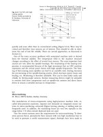
As was mentioned before, the machining process normally takes place under
high-stress, high-strain rate and high-temperature conditions with various kinds
of external disturbances including the cutting and grinding fluids. It is therefore
understood that high reliability and stability against various kinds of disturbances
are the most important requirements for the sensors in addition to the basic per-
formance and accuracy of the transducers. According to the answers given by in-
dustry engineers to the questionnaire concerning tool condition monitoring [2],
the importance of technical criteria in selecting the sensors is in the order (1) reli-
ability against malfunctioning, (2) reliability in signal transmission, (3) ease of in-
stallation, (4) life of the sensor, and (5) wear resistance of the sensor.
The importance of items in evaluating the monitoring system is also given in
the order (1) reliability against malfunctions, (2) performance to cost ratio, (3) in-
formation obtained by the sensor, (4) speed of diagnosis, (5) adaptability to
changes of process, (6) usable period, (7) ease of maintenance and repair, (8) level
of automation, (9) ease of installation, (10) standard interface, (11) standardized
user interface, (12) completeness of manuals, and (13) possibility of additional
functions.
Table 1.3-4 summarizes items to be considered generally in selecting transdu-
cers and the sensors. It is basically desirable to implement on-line, in-process,
continuous, non-contact, and direct sensing, but it is generally difficult to satisfy
all of these requirements. The property of the object is directly sensed in the case
of direct sensing, whereas in the case of indirect sensing it is estimated indirectly

from other properties which can be easily measured and are related to the prop-
erty to be measured. It should be noted that the property of object to be estimated
indirectly must have a good correlation with the property to be measured. Indirect
sensing is useful and is widely adopted when direct sensing is difficult.
1 Fundamentals30
Fig. 1.3-7 Relation of input and output at some typical frequencies
A typical indirect sensing is to estimate the wear and damage of a tool by sen-
sing the cutting and grinding forces, the cutting temperature, the vibration, or the
sound emitted. The wear and damage of the tool have a good correlation with
those properties mentioned above, but they are also dependent on other condi-
tions, such as the cutting and grinding conditions including the speed, the depth
of cut and the feed, the cutting and grinding modes, the tool materials, etc. It is
therefore necessary to have a good understanding of the correlation among the
properties and the influencing factors.
1.3.4
Boundary Conditions
Sensing of the state of the machining process, the tool, the work, and the ma-
chine tool is not easy and it is restricted by many factors, as was mentioned ear-
lier. Difficulties encountered in sensing, which are boundary and restrictive condi-
tions for sensing, and their typical examples are summarized in Table 1.3-5. The
most important requirements for sensing are to obtain the necessary information
as accurately as possible under unfavorable conditions without disturbing the ma-
chining process, which normally takes place under high stress, high strain rate
and high temperature.
It is always desirable to sense the properties of the object directly in-process
and on-line, which is not generally easy to realize. When the cutting/grinding
temperature and the acoustic emission (AE) signal are sensed, the sensors are
normally attached apart from the cutting/grinding region, and hence the quality
of necessary information deteriorates while the heat and the ultrasonic vibration
are transmitted. It is more difficult to sense such signals when the transmission

path is discontinuous, such as in the case of a rotating spindle or moving table.
Fluid coupling is employed in the case of ultrasonic vibration.
The signal transmission is still difficult when the transducers are located on the
rotating spindle or the moving table, even after the signals to be transmitted are
converted to an electric signal by the transducers. The slip ring, wireless transmis-
sion with use of radio waves and the optical methods are commonly employed in
such cases.
1.3 Sensors in Mechanical Manufacturing 31
Tab. 1.3-4 Items to be considered in selecting sensors
In-process sensing; between-process sensing; post-process sensing
On-line sensing; on-machine sensing; off-line sensing
Continuous sensing; intermittent sensing
Direct sensing; indirect sensing
Active sensing; passive sensing
Non-contact sensing; contact sensing
Proximity sensing; remote sensing
Single sensor; multi-sensor
Multi-functional sensor; single-purpose sensor
Another difficulty is that the sensors and the sensing systems are generally re-
quired to sense the properties of objects even though the combinations of the cut-
ting/grinding methods, the machining conditions, the tool material, the work
material, and even the machine itself are altered. In this sense, versatility is im-
portant for the sensors and the sensing systems.
1.3.5
Signal Processing and Conversion
1.3.5.1 Analog Signal Processing
The property of the object to be sensed is transformed into voltage, current, elec-
trical charge, or other signal by the transducer. The signals other than the voltage
signal are generally further transformed into a voltage signal which is easier to
handle. The analog voltage signal is generally filtered to eliminate unnecessary

frequency components and amplified prior to the digitization in order to be pro-
cessed by computer.
There are basically two types of analog filters, the low-pass filter and the high-
pass filter. The low-pass filter passes the signal containing the frequency compo-
1 Fundamentals32
Tab. 1.3-5 Difficulties in sensing and examples
Items of difficulty Example
In-process/on-line sensing is difficult Geometrical and dimensional accuracy of work
Surface roughness and quality of work
Wear and damage of tool
Thermal deformation of machine
Direct sensing is difficult Tool wear and damage in continuous cutting
Thermal deformation of machine
Distance between object and sensing position
is large
Cutting/grinding point versus position where
sensors can be placed
Installation of sensor should not affect machin-
ing process and rigidity of machining system
Reduction of rigidity of tool or machine ele-
ments to measure force by strain
Environment is not clean Existence of cutting fluid
Electrical noise due to power circuit
Signal is to be transmitted via rotating or
moving element
Signal transmission from rotating spindle or
fast-moving table
Signal transmission via rotatable tool turret
Complicated correlation exists among many
factors

Property of object to be sensed are affected by
machining conditions, tool material, work ma-
terial, etc.
Variety of machining method is large Sensors are required to be effective for different
machining methods, such as tapping, drilling,
end milling, face milling, etc. on one machine
nents below the predetermined frequency, named the cut-off frequency, and prohi-
bits the signal containing the frequency components above the cut-off frequency.
The low-pass filter is commonly used when the high-frequency noise compo-
nents, especially the electric noise components, are to be eliminated.
The high-pass filter passes the signal containing the frequency components
above the cut-off frequency and prohibits the signal containing the frequency
components below the cut-off frequency. The high-pass filter is commonly used
when the AC (alternating current) components of the signal are utilized and the
DC (direct current) components and the low-frequency components are elimi-
nated. In other words, it is used when the dynamic components of the signal are
utilized and the static or the low-frequency components are eliminated.
The combination of the low-pass and the high-pass filters constitutes the band-
pass filter and the band-reject filter. The band-pass filter passes only the signal
containing the frequency components within the specified frequency range,
whereas the band-reject filter prohibits the signal containing the frequency com-
ponents of that frequency range.
The band-pass filter is commonly used when the signal components of a partic-
ular frequency range are utilized, such as in the case when the signal compo-
nents synchronizing to the rotational frequency of the spindle or the engagement
of the milling cutter are to be monitored. The band-reject filter is used when the
signal components of a particular frequency range are to be omitted.
The frequency characteristics of the filters are shown schematically in Fig-
ure 1.3-8 in terms of the output/input ratio. It should also be noted that the phase
information is distorted when the signal is passed through the filters as shown in

Figure 1.3-6.
1.3 Sensors in Mechanical Manufacturing 33
Fig. 1.3-8 Frequency characteristics
of filters
The other transformation and processing of analog signals include the differen-
tiation, integration, and logarithmic transformation, which are summarized in Ta-
ble 1.3-6. The displacement signal can be transformed to a velocity signal by dif-
ferentiation, and further to an acceleration signal, and vice versa. These signal
transformations are often carried out after the signal is converted to a digital sig-
nal, which is explained below.
1.3.5.2 AD Conversion
The analog time series of electric signals is generally converted into digital values
by the AD (analog-to-digital) converter prior to processing by computer. The im-
portant parameters of the AD converter are the input range, the number of digits
of conversion, the sampling time, and the total number of sampled data (Ta-
ble 1.3-7). The AD converter equally divides the voltage of the input range into the
given digits and gives the corresponding number to the input voltage at a given
sampling interval Dt. Comparison of the original analog signal and digitized sam-
ples is illustrated schematically in Figure 1.3-9.
When the input range of an 8-bit AD converter is ± 1 V, the signal from +1 V to
–1 V is converted to digital numbers from +127 to –127. This means that the elec-
tric signal is digitized with a resolution of 7.9 mV, or 1/127 V. The signal of 0.1 V
is converted to 13, 0.5 V to 64, and so forth. The commonly used digits other
than 8 bits are 10 bits (±511), 12 bits (±2047) and 16 bits (± 8191). The AD con-
version is always associated with the digitization error, but it can be ignored in
practice if the number of digits is chosen to be high enough.
It is easily understood that the resolution of AD conversion is better if the num-
ber of digits is larger. However, it is useless to increase the resolution beyond the
noise level of the original analog signal. The input signal is to be properly ampli-
fied prior to the AD conversion in such a way that the maximum voltage expected

matches the input range of the AD converter.
1 Fundamentals34
Tab. 1.3-6 Typical processing and transformation of analog signal
Filtering (low-pass, high-pass, band-pass, band-reject)
Amplification
Differentiation
Integration
Logarithmic transformation
Tab. 1.3-7 Important parameters in AD conversion
Range of analog signal input
Number of digit (or resolution)
Sampling time Dt
Total number of sampled data M
Maximum frequency f
max
= 1/2Dt
Frequency resolution Df =1/MDt
The sampling time Dt gives the time interval of successive AD conversion. A
sampling time of 1 ms means that the signal is converted at a sampling rate of
1000 samples per second, or a sampling frequency of 1 kHz. If the sampling time
is shorter or the sampling frequency is higher, the original signal can be better re-
presented in a digital form, but the total number of digital data M for a given
time period becomes larger and may require a longer processing time.
The sampling time Dt gives the upper limit frequency f
max
of the digitized sig-
nal to be analyzed, or
f
max
 1=2 Dt1:3-1

This means that the frequency range of the digitized signal is limited below 1/
(2 Dt) Hz, and the frequency components of the original analog signal beyond this
frequency are included in the frequency components of the digitized signal which
is lower than f
max
. This is called Shannon’s sampling theorem.
An example of the case of a low sampling rate as compared with the frequency
component of the original analog signal is depicted in Figure 1.3-10. It is under-
stood that an original sinusoidal analog signal sampled at a sampling frequency
lower than its frequency is represented as a low-frequency signal in digitized
form. The signal components with frequencies beyond f
max
are thus represented
as components at lower frequencies in digital form. This phenomenon is called
aliasing or folding.
1.3 Sensors in Mechanical Manufacturing 35
Fig. 1.3-9 Schematic illustration of AD conversion
Fig. 1.3-10 Example of low sampling rate
Dt: Sampling time:
In order to avoid such problems, an analog low-pass filter is generally employed
prior to AD conversion, the cut-off frequency of which is matched to the sampling
time. Another method is to employ digital filtering, which is a digital calculation
equivalent to analog filtering. The original analog signal is sampled at a sampling
frequency high enough to avoid folding, processed by the digital processor to elim-
inate the high-frequency components and then sampled again at a predetermined
sampling frequency which is much lower than the original sampling frequency.
When two or more analog signals are to be digitized simultaneously, it is im-
portant that the signal of each channel must be sampled at the same time with-
out any delay. This is realized either by employing several AD converters operated
in synchronization, or employing the sample and hold circuits, which practically

freezes the levels of the analog signals while the single AD converter scans all the
analog signals and converts them into digital data.
1.3.5.3 Digital Signal Processing
Once the sensor signal has been converted into digital data, the latter are pro-
cessed in many ways to extract the features and to give the basis for the identifica-
tion and the decision making in the following process. Most of the signal data
coming from the sensor are time series data, and they are primarily processed in
the time domain or in the frequency domain after Fourier transformation. The
multi-dimensional data, such as the image data, are treated as they are, or some
distinctive features extracted from the image are utilized. Some typical methods
of signal processing are summarized in Table 1.3-8. The wavelet transform is a
1 Fundamentals36
Tab. 1.3-8 Typical signal processing methods and distinctive values
Domain of signal processing Method of signal processing Distinctive value
Time domain Selection of distinctive feature
Time series analysis
Correlation analysis
Peak value
Rms value
Differentiated value
Integrated value
Duration
Filtered value
Moving average
Frequency
Accumulated frequency
Auto-correlation
Cross-correlation
Difference in arrival time
Frequency domain DFT (digital Fourier transform) Band power

Power spectrum
Cross spectrum
Cepstrum
Phase (difference)
Others Wavelet transform
Image processing
Wavelet
Pattern (image data)
new method which deals with the changes in the frequency characteristics of the
signal. Some typical signal processing methods are explained below.
Let the digitized time series data of analog signal x(t) be represented as x(i),
where i is an integer and
t  iDt 1:3-2
The moving average MA(i)ofx(i) is given by
MAi
1
K
X
KÀ1
j0
ajxi À j1:3-3
where a(j) are coefficients normally chosen to be 1. The range of integration is
sometimes chosen to be from j =–K to j = K.
The algorithm of digital filtering mentioned above is practically the same as
Equation (1.3-3). The function of the filter can be low-pass or high-pass depend-
ing on the coefficients of a(j).
For a given set of time series data of x(i)(i =0,1,2, ,M–1), the auto-correla-
tion function of x(i) is given by
C
xx

k
1
M
X
MÀkÀ1
i0
x k  ixik  0; 1; ; h1:3-4
The cross-correlation function between x(i) and y(i) is given in the same way by
C
xy
k
1
M
X
MÀkÀ1
i0
x k  iyik  0; 1; ; h1:3-5
C
xy
k
1
M
X
MÀ1
iÀk
x k  iyik À1; ; Àh1:3-6
The Fourier transform of x(i) is given by
Xj2pk=MDt
X
MÀ1

i0
x i expÀj2pki=M1:3-7
where k =0,1,2, ,M/2.
The discrete spectrum X(j2pk/MDt) is given at discrete frequencies f = k/MDt.
This means that the frequency resolution is given by dividing the maximum fre-
quency f
max
by M/2, as was shown in Equation (1.3-1) the maximum frequency is
determined by the sampling time Dt and is given by 1/2Dt. The frequency resolu-
tion Df of the digitized data is then given by
Df  1=MDt  1=T 1:3-8
where T is the observation period of the signal.
1.3 Sensors in Mechanical Manufacturing 37
In order to improve the frequency resolution and make Df small, it is necessary
to increase the number M or the observation period of the signal or to increase
the sampling time Dt. The selection of sampling time Dt is restricted by the
upper limit frequency or the maximum frequency, as explained before.
The Fourier spectrum X(j2 p k/MDt) is a complex number, and it is divided into
the real and the imaginary parts as
ReXA
k

X
MÀ1
i0
x i cos 2pki=Mk  0; 1; ; M=21:3-9
ImXB
k

X

MÀ1
i0
x i sin 2pki=Mk  1; 2; ; M=21:3-10
The relation between the original time series and the Fourier transform is shown
schematically in Figure 1.3-11. The power spectrum P
k
at a frequency f =k/MDt is
given by
P
k
A
2
k
 B
2
k

1=2
1:3-11
1 Fundamentals38
Fig. 1.3-11 Relation of time series data and its Fourier spectra
Df
NDT
2DT
Df=max
Dt
(N–1)Dt
Df=fmax
1.3.6
Identification and Decision Making

1.3.6.1 Strategy of Identification and Decision Making
The digitized sensor signals are used to extract their features, identify the state of
the machining process and the conditions of the tool, the work, the machine, etc.,
and then make decisions to take necessary actions when it is necessary.
Figure 1.3-12 shows typical input-output relations between the input sensor sig-
nal and the output which is the status identified. In most cases, a single input sig-
nal is utilized to identify the specific state of the system, such as the condition of
the tool as shown in case (a). Some sensor signals, such as the vibration signal or
the force signal, contain information of various kinds of status, such as the tool
wear, the chatter vibration, etc., and hence are utilized to identify those conditions
as in case (b).
In order to increase the reliability of identification under varying conditions or
to avoid the uncertainty in the identified results, it is useful to use several input
signals instead of using a single input signal as in cases (c) and (d). Various kinds
of algorithms or rules can be applied to the input signals. Such fusion of the in-
put signals is becoming more popular to increase the quality of the identification.
The distinctive values of the processed signals, the extracted features or the
identified parameters are mostly compared with the predetermined or given
thresholds to identify the status by referring to these threshold values. In order to
guarantee high accuracy of the identification, a reliable database must be prepared
in advance based on the actual tests, etc. However, it is not easy to do so, as there
are many combinations of the machining conditions, the tool, and the work, and
this makes the identification difficult.
Another approach to identification is so-called model-based identification. Var-
ious kinds of analytical models or empirical models are employed which utilize
1.3 Sensors in Mechanical Manufacturing 39
Fig. 1.3-12 Input-output relation
of identification
the known information, such as the cutting conditions. For instance, the general-
ized model parameters are extracted from the input signals and are compared

with the database, or the hypothetical output of the system is calculated which is
to be compared with the actual signal data. It is expected that both the reliability
and the versatility of identification will be increased by introducing the model-
based approach. The differences between the above two approaches of identifica-
tion are shown schematically in Figure 1.3-13.
The final decision is made based on the results of the identification. Typical de-
cisions made or actions to be taken in the case of machining are summarized in
Table 1.3-9. When the abnormal state is identified, the machine is either to be
stopped or continues to operate depending on the nature of the abnormal state
and the control capability of the machine.
Various kinds of AI (artificial intelligence) technologies are applied to the identi-
fication and the decision making, which are briefly explained below.
1.3.6.2 Pattern Recognition
The pattern recognition method has been widely applied to identify the state of
the machining process and the cutting tool, etc. [3–5].
It is based on the similarity between a sample to be identified and the patterns
or classes that describe the target statuses. From a geometrical point of view, the
monitoring indices, or the selected distinctive feature values extracted from the
1 Fundamentals40
Tab. 1.3-9 Typical decisions made and actions to be taken
Emergency stop or feed stop, and
· change tool
· dress grinding wheel
· change conditions (including NC program)
to avoid chatter vibration, other damage, etc.
· notify the operator
Continue operation but change
· spindle speed
· feed speed
· cutter path to compensate tool wear, thermal

deformation or other error source
Fig. 1.3-13 Two approaches
of identification
sensed signals, x =(x
1
, x
2
, , x
m
) span an m-dimensional space. In the span, each
target status, h
j
, is characterized by a pattern vector p
j
=(p
j1
, p
j2
, , p
jm
). The simi-
larity between the sample with the feature values and a pattern is measured by
the distance between the two vectors. The minimum distance is then used as the
criterion for classifying the sample.
The clustering of the sample points, which belong to the particular patterns, is
accomplished by a proper coordinate transformation in such a way that the mean
square of the above mentioned distance becomes minimum. The transformed sig-
nal x’ is given by
x
H

wx 1:3-12
where [w] is the transformation matrix.
Figure 1.3-14 shows schematically how the original sample points are classified
into distinctive classes by a proper transformation in a two-dimensional space.
The most appropriate coordinate transformation is obtained by learning with given
sample data.
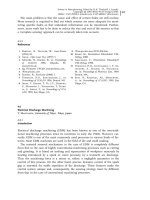
1.3.6.3 Neural Networks
The neural network is basically an imitation of the neural system of animals, and
it has been applied to identify the state of the cutting tool [6], the machining pro-
cess [7, 8], and also the thermal deformation of the machine tool [9], etc. The ad-
vantages of neural networks over pattern recognition are that it can easily consti-
tute optimum nonlinear multi-input functions for pattern recognition and that
the accuracy of pattern recognition is easily improved by learning.
A neural network may consist of several layers and each layer has a number of
neurons as shown in Figure 1.3-15. The output O
j
L
of the jth unit in the Lth layer
to its input X
j
L
is generally given by
O
L
j
 hX
L
j
À 
L

j
1:3-13
where h
j
L
is the threshold value. The well-known sigmoid monotonic input-output
relation is generally adopted, which is given by
hX
L
j
À 
L
j

1
1  1= expX
L
j
À 
L
j

1:3-14
1.3 Sensors in Mechanical Manufacturing 41
Fig. 1.3-14 Separation of clusters
by coordinate transformation
The input X
j
L
of the jth unit in the Lth layer, except the input layer, is given by the

weighted sum of the outputs from the units in the previous layer, or
X
L
j

X
m
i1
W
LÀ1
ji
O
LÀ1
i
1:3-15
where W
ji
L–1
represents the weight which is given by the path from ith unit in the
(L–1)th layer to the jth unit in the Lth layer, and m is the number of nodes in the
(L–1)th layer.
The outputs of the network O
k
are calculated based on the inputs following the
paths of the network and the procedures mentioned above. The thresholds h and
the weights W are so determined that the sum of squares of the differences be-
tween the ideal outputs R
k
and the calculated outputs O
k

is minimized, or
X
L
j

X
m
k1
R
k
À O
k

2
1:3-16
is minimized. The thresholds and the weights are further modified through learn-
ing as the additional data are given to the network.
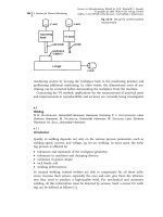
1.3.6.4 Fuzzy Reasoning
Fuzzy reasoning was first introduced by Zadeh [10] and has been applied to state
identification and decision making when there exists fuzziness in the process,
such as the grinding process [11].
Fuzzy reasoning is a reasoning method based on the fuzzy production rules.
The fuzzy production rules are given in such a way as
1 Fundamentals42
Fig. 1.3-15 Basic structure of neural network
IF x
1
is very small and x
2
is medium

THEN x
k
is small
In the fuzzy approach, uncertain events are described by means of a fuzzy degree
or a membership function. If A is an uncertain event as a function of x, A can be
described by
A fxjl
A
xg 1:3-17
where l
A
(x) the membership function. The membership function is a monoto-
nous function 0£ l
A
(x) £ 1, while ‘0’ means certainly no and ‘1’ means certainly
yes. Some typical examples of the membership functions are shown in Figure 1.3-
16, which represent the linguistic variables, such as VS (very small), S (small), M
(medium), L (large) and VL (very large).
When a set of the input variables are given, the degrees of applicability of the
rules are calculated according to the membership functions and they are applied
to the production rules to give the quantified outputs. The detailed procedures of
the fuzzy reasoning and examples of applications are given in Ref. [12].
Other AI technologies, such as expert systems, are employed for state identifica-
tion, diagnosis, and decision making, but they are not explained in detail here.
1.3.7
Communication and Transmission Techniques
Communication and transmission of the signal within the sensing system are
generally processed in digital form after digitization of the analog input signal.
The analog transmission of the sensed signal prior to digitization requires special
care, as the quality of the signal transmission directly influences the quality of

sensing. The analog signal is easily deteriorated by the noise signal surrounding
the transducers/sensors and the signal transmission cables. The high-frequency
noise signals coming from the power circuits including the motors, the digital de-
vices, etc., as well as those coming from the power supply can be major sources
of noise signals.
The signal transmission requires special techniques when the signal is to be
transmitted via relatively moving interfaces without contact. The slip ring, wire-
1.3 Sensors in Mechanical Manufacturing 43
Fig. 1.3-16 Typical examples of membership
functions
Value of variable
less transmission with use of radio waves and optical methods are generally em-
ployed in such cases.
The communication and transmission of digital signals and data can be easily
conducted with the aid of current computer technology. A large amount of digital
data can be transmitted between the I/O (input/output) devices and computers via
an RS232C or RS422 serial interface at high speeds. Most computers and control-
lers are connected via the ether-net with the TCP/IP protocol, and the messages
and the data can be easily transmitted with use of appropriate communication
programs.
The internet services are available to transmit messages and data all over the
world via a dedicated line or a commercial telephone line.
1.3.8
Human-Machine Interfaces
The outputs of the sensing system, which are the processed sensor signals, the
identified states of the process or the system, or the decisions made, are trans-
mitted to the machine controller and to the operator. At the same time, the opera-
tor has to input various kinds of commands to the sensing system. In this sense
the human-machine interface plays an important role in the sensing system.
Typical I/O devices or media between the sensing system and the operators are

listed in Table 1.3-10. The operators can input commands via dedicated switches
or a keyboard, which is more versatile. A touch panel is widely adopted on the ac-
tual production floor, which is used to input commands by pressing the specified
location on the screen displaying the various functions. The information from the
pressed position on the screen is input into the computer via the touch sensor
and transformed to a command input. Voice commands are not widely used in
noisy environments.
Alarms are the most popular output to the operator when some malfunctions
are identified in the system. The visual output, either a graphical presentation or
a document, via the display, helps the operator to understand the situation. Oral
output with use of a synthetic voice is also helpful.
1 Fundamentals44
Tab. 1.3-10 Typical input/output devices or media
Input devices/media Output devices/media
Switch
Keyboard
Touch panel
Voice command
Alarm (sound, light, etc.)
Voice (synthetic voice)
Display
Printout
1.3 Sensors in Mechanical Manufacturing 45
1.3.9
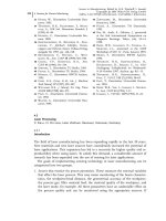
References
1 Technical Committee on Integrated
Manufacturing Systems, Questionnaire
on Unmanned Operation and Cutting State
Monitoring; JSPE Technical Committee on
IMS, 1980 (in Japanese).

2 Moriwaki, T., Result of Questionnaire on
Tool Condition Monitoring. Activity Report
of Technical Committee on IMS; JSPE,
1994, pp. 58–68.
3 Monostori, L., Comput. Ind. 7 (1986) 53–
64.
4 Moriwaki, T., Tobito, M., Trans. ASME J.
Engl. Ind. 112 (1990) 214–218.
5 Du, R. et al., Trans. ASME J. Engl. Ind.
117 (1995) 121–132.
6 Dornfeld, D., Ann. CIRP 39(1) (1990)
101–105.
7 Moriwaki, T., Mori, Y., in: Mechatronics
and Manufacturing Systems; Amsterdam:
North-Holland, 1993, pp. 497–502.
8 Du, R. et al., Trans. ASME J. Eng. Ind.
117 (1995) 133–141.
9 Moriwaki, T., Zhao, C., in: Proceedings of
IFIP TC5/WG5.3, 8th International PRO-
LAMAT Conference; 1992, pp. 685–697.
10 Zadeh, L. A., Trans. IEEE SMC-3 (1973)
28.
11 Sakakura, M., Inasaki, I., Ann. CIRP
42(1) (1993) 379–382.
12 Mamdani, E. H., Gaines, B.R., Fuzzy Rea-
soning and Its Applications; New York: Aca-
demic Press, 1981.