Tài liệu Modeling, Measurement and Control P11 ppt
Bạn đang xem bản rút gọn của tài liệu. Xem và tải ngay bản đầy đủ của tài liệu tại đây (4.78 MB, 16 trang )
181
II
Vibration Control
Nejat Olgac
8596Ch10Frame Page 181 Monday, November 12, 2001 12:04 PM
© 2002 by CRC Press LLC
11
Active Damping of
Large Trusses
11.1 Introduction
11.2 Active Struts
Open-Loop Dynamics of an Active Truss • Integral
Force Feedback • Modal Damping • Experimental
Results
11.3 Active Tendon Control
Active Damping of Cable Structures • Modal
Damping • Active Tendon Design • Experimental
Results
11.4 Active Damping Generic Interface
11.5 Microvibrations
11.6 Conclusions
Abstract
This chapter reviews various ways of damping large space trusses. The first part discusses the use
of active struts consisting of a piezoelectric actuator collocated with a force sensor. The guaranteed
stability properties of the integral force feedback are reviewed and the practical significance of the
modal fraction of strain energy is stressed. The second part explains the concept of active tendon
control of trusses; the similarity of this concept with the previous one is pointed out. The third part
describes an active damping generic interface based on a Stewart platform architecture with
piezoelectric legs. The similarity with the previous concepts is emphasized. Finally, the damping
of microvibrations is briefly discussed.
11.1 Introduction
The development of future generations of ultralight and large space structures will probably not
be possible without active damping enhancement of the structures and active isolation of the
scientific payloads that are sensitive to vibrations. Interferometric missions are an example partic-
ularly stringent geometric stability requirements.
1,2
This chapter addresses the problem of active
damping of large trusses with three different concepts: (i) active strut, (ii) active tendon, and (iii)
generic interface. In all cases, the same control architecture is used: a collocated piezoelectric
actuator and force sensor connected by a local controller with an integral force feedback (IFF).
11.2 Active Struts
The first concept is the most natural; it consists of replacing some passive bars in the truss by active
struts (Figure 11.1). The active struts consist of a piezoelectric linear actuator (or another type of
A. Preumont
Université Libre de Bruxelles
Frederic Bossens
Université Libre de Bruxelles
Nicolas Loix
Micromega Dynamics
8596Ch11Frame Page 181 Tuesday, November 6, 2001 10:12 PM
© 2002 by CRC Press LLC
linear displacement actuator such as magnetostrictive) co-linear with a force transducer. This
concept was first demonstrated in the late 1980s.
3-6
11.2.1 Open-Loop Dynamics of an Active Truss
Consider the active truss of Figure 11.2. when a voltage
V
is applied to an unconstrained linear
piezoelectric actuator, it produces an expansion
δ
.
(11.1)
where
d
33
is the piezoelectric coefficient,
n
is the number of piezoelectric ceramic elements in the
actuator;
g
a
is the actuator gain. This equation neglects the hysteresis of the piezoelectric expansion.
If the actuator is placed in a truss, its effect on the structure can be represented by equivalent
piezoelectric loads acting on the passive structure. As for thermal loads, the pair of self-equilibrating
piezoelectric loads applied axially to both ends of the active strut (Figure 11.2) has a magnitude
equal to the product of the stiffness of the active strut,
K
a
, by the unconstrained piezoelectric
expansion
δ
:
(11.2)
FIGURE 11.1
Active truss with piezoelectric struts (ULB).
δ= =dnV gV
a33
pK
a
=δ
8596Ch11Frame Page 182 Tuesday, November 6, 2001 10:12 PM
© 2002 by CRC Press LLC
Assuming no damping, the equation governing the motion of the structure excited by a single
actuator is
(11.3)
where
b
is the influence vector of the active strut in the global coordinate system. The nonzero
components of
b
are the direction cosines of the active bar. As for the output signal of the force
transducer, it is given by
(11.4)
where
δ
e
is the elastic extension of the active strut, equal to the difference between the total extension
of the strut and its piezoelectric component
δ
. The total extension is the projection of the displace-
ments of the end nodes on the active strut,
∆
= b
T
x
. Introducing this into Equation (11.4), we get
(11.5)
Note that because the sensor is located in the same strut as the actuator, the same influence vector
b
appears in the sensor Equation (11.5) and the equation of motion (11.3). If the force sensor is
connected to a charge amplifier of gain
g
s
, the output voltage
v
o
is given by
(11.6)
Note the presence of a feedthrough component from the piezoelectric extension
δ
. Upon trans-
forming into modal coordinates, the frequency response function (FRF)
G
(
ω
) between the voltage
V
applied to the piezo and the output voltage of the charge amplifier can be written:
7
(11.7)
FIGURE 11.2
Active truss. The active struts consist of a piezoelectric linear actuator colinear with a force
transducer.
Mx Kx bp bK
a
˙˙
+==δ
yT K
ae
== δ
yT Kbx
a
T
== −()δ
vgTgKbx
ssa
T
0
== −()δ
v
V
GggK
sa a
i
i
i
n
0
22
1
1
1==
−
−
=
∑
()
/
ω
ν
ωΩ
8596Ch11Frame Page 183 Tuesday, November 6, 2001 10:12 PM
© 2002 by CRC Press LLC
where
Ω
i
are the natural frequencies, and we define
(11.8)
The numerator and the denominator of this expression represent, respectively, twice the strain
energy in the active strut and twice the total strain energy when the structure vibrates according to
mode
i
.
ν
i
(
≥
0) is, therefore, called the
modal fraction of strain energy
in the active strut. From
Equation (11.7), we see that
ν
i
determines the residue of mode
i
, which is the amplitude of the
contribution of mode
i
in the transfer function between the piezo actuator and the force sensor. It
can, therefore, be regarded as a compound index of controllability and observability of mode
i
.
ν
i
is readily available from commercial finite element programs and can be used to select the proper
location of the active strut in the structure: the best location is that with the highest
ν
i
for the modes
that we wish to control.
5
11.2.2 Integral Force Feedback
The FRF (Equation 11.7) has alternating poles and zeros (Figure 11.3) on the imaginary axis (or
near if the structural damping is taken into account); on the other hand,
G
(
ω
) has a feedthrough
component and some roll-off must be added to the compensator to achieve stability. It is readily
established from the root locus (Figure 11.4) that the positive integral force feedback (IFF):
(11.9)
is unconditionally stable for all values of
g
. The negative sign in Equation (11.9) is combined with
the negative sign in the feedback loop (Figure 11.5) to produce a positive feedback.
In practice, it is not advisable to implement plain integral control, because it would lead to
saturation. A forgetting factor can be introduced by slightly moving the pole of the compensator
from the origin to the negative real axis, leading to
(11.10)
FIGURE 11.3
Open-loop FRF
G
(
ω
) of the active truss (a small damping is assumed).
ν
φ
µ
φ
φφ
i
a
T
i
ii
a
T
i
i
T
i
Kb Kb
K
==
() ()
2
2
2
Ω
gD s
g
Ks
a
()=
−
gD s
g
Ks
a
()
()
=
−
+ε
8596Ch11Frame Page 184 Tuesday, November 6, 2001 10:12 PM
© 2002 by CRC Press LLC
This does not affect the general shape of the root locus and prevents saturation. Note that piezo-
electric force sensors have a built-in high-pass filter.
11.2.3 Modal Damping
Combining the structure Equation (11.3), the sensor Equation (11.5), and the controller Equation
(11.9), the closed-loop characteristic equation reads
(11.11)
From this equation, we can deduce the open-loop transmission zeros, which coincide with the
asymptotic values of the closed-loop poles as
g
→
∞
. Taking the limit, we get
(11.12)
which states that the zeros (i.e., the anti-resonance frequencies) coincide with the poles (resonance
frequencies) of the structure where the active strut has been removed (corresponding to the stiffness
matrix
K-bK
a
b
T
)
.
To evaluate the modal damping, Equation (11.11) must be transformed in modal coordinates
with the change of variables
x =
Φ
z
. Assuming that the mode shapes have been normalized
according to
Φ
T
M
Φ
= I
and taking into account that
Φ
T
K
Φ
= diag
(
Ω
i
2
)
=
Ω
2
, we have
FIGURE 11.4
Root locus of the integral force feedback.
FIGURE 11.5
Block diagram of the integral force feedback.
Ms K
g
sg
bK b x
a
T2
0+−
+
()
=
Ms K bK b x
a
T2
0+−
[]
=()
8596Ch11Frame Page 185 Tuesday, November 6, 2001 10:12 PM
© 2002 by CRC Press LLC
(11.13)
The matrix
Φ
T
(
bK
a
b
T
)
Φ
is, in general, fully populated. If we assume that it is diagonally
dominant, and if we neglect the off-diagonal terms, it can be rewritten
(11.14)
where
ν
i
is the fraction of modal strain energy in the active member when the structure vibrates
according to mode
i
;
ν
i
is defined by Equation (11.8). Substituting Equation (11.14) into
Equation (11.13), we find a set of decoupled equations
(11.15)
and, after introducing
(11.16)
it can be rewritten
(11.17)
By comparison with Equation (11.11), we see that the transmission zeros (the limit of the closed-
loop poles as
g
→∞
) are
±
j
ω
i
. The characteristic equation can be rewritten
(11.18)
The corresponding root locus is shown in Figure 11.6. The depth of the loop in the left half plane
depends on the frequency difference
Ω
i
–
ω
i
, and the maximum modal damping is given by
FIGURE 11.6
Root locus of the closed-loop pole for the IFF.
Is
g
sg
bK b z
T
a
T22
0+−
+
=ΩΦ Φ()
ΦΦΩ
T
a
T
ii
bK b() ()≈ diag ν
2
s
g
sg
iii
22 2
0+−
+
=ΩΩν
ων
ii i
22
1=−Ω ()
s
g
sg
iii
22 22
0+−
+
−
()
=ΩΩω
10
22
22
+
+
+
=g
s
ss
i
i
()
()
ω
Ω
8596Ch11Frame Page 186 Tuesday, November 6, 2001 10:12 PM
© 2002 by CRC Press LLC
(11.19)
It is obtained for . For small gains, it can be shown that
(11.20)
This interesting result tells us that, for small gains, the active damping ratio in a given mode is
proportional to the fraction of modal strain energy in the active element. This result is very useful
for the design of active trusses; the active struts should be located to maximize the fraction of
modal strain energy
ν
i
in the active members for the critical vibration modes. The preceding results
have been established for a single active member. If several active members are operating with the
same control law and the same gain
g
, this result can be generalized under similar assumptions. It
can be shown that each closed-loop pole follows a root locus governed by Equation (11.18) where
the pole
Ω
i
is the natural frequency of the open-loop structure and the zero
ω
i
is the natural frequency
of the structure where the active members have been removed.
11.2.4 Experimental Results
Figures 11.7 and 11.8 illustrate typical results obtained with the test structure of Figure 11.1. The
modal damping ratio of the first two modes is larger than 10%. Note that in addition to being
simple and robust, the control law can be implemented in an analog controller, which performs
better in microvibrations.
11.3 Active Tendon Control
The use of cables to achieve lightweight spacecrafts is not new; it can be found in Herman Oberth’s
early books
17,18
on astronautics. In terms of weight, the use of guy cables is probably the most
efficient way to stiffen a structure. They also can be used to prestress a deployable structure and
eliminate the geometric uncertainty due to the gaps. One further step consists of providing the
cables with active tendons to achieve active damping in the structure. This approach has been
developed in References 7–12.
FIGURE 11.7
Force signal from the two active struts during the free response after impulsive load.
ξ
ω
ω
i
ii
i
max
=
−Ω
2
g
iii
=Ω Ω / ω
ξ
ν
i
i
i
g
=
2Ω
8596Ch11Frame Page 187 Tuesday, November 6, 2001 10:12 PM
© 2002 by CRC Press LLC
11.3.1 Active Damping of Cable Structures
When using a displacement actuator and a force sensor, the (positive) integral force feedback
Equation (11.9) belongs to the class of “energy absorbing” controls: indeed, if
(11.21)
the power flow from the control system is . This means that the control can
only extract energy from the system. This applies to nonlinear structures as well; all the states
which are controllable and observable are asymptotically stable for all positive gains (infinite gain
margin). The control concept is represented schematically in Figure 11.9 where the spring-mass
system represents an arbitrary structure. Note that the damping introduced in the cables is usually
very low, but experimental results have confirmed that it always remains stable, even at the
parametric resonance, when the natural frequency of the structure is twice that of the cables.
Whenever possible, however, the tension in the cables should be adjusted in such a way that their
first natural frequency is above the frequency range where the global modes must be damped.
FIGURE 11.8
FRF between a force in A and an accelerometer in B, with and without control.
FIGURE 11.9
Active damping of cable structures.
δ ~ Tdt
∫
WT T=− − ≤
˙
~δ
2
0
8596Ch11Frame Page 188 Tuesday, November 6, 2001 10:12 PM
© 2002 by CRC Press LLC
11.3.2 Modal Damping
If we assume that the dynamics of the cables can be neglected and that their interaction with the
structure is restricted to the tension in the cables, and that the global mode shapes are identical
with and without the cables, one can develop an approximate linear theory for the closed-loop
system. The following results that follow closely those obtained in the foregoing section (we assume
no structural damping) can be established:
The open-loop poles are
±
j
Ω
i
where
Ω
i
are the natural frequencies of the structure including
the active cables and the open-loop zeros are
±
j
ω
i
where
ω
i
are the natural frequencies of the
structure where the active cables have been removed.
If the same control gain is used for every local control loop, as
g
goes from
0 to ∞, the closed-
loop poles follow the root locus defined by Equation (11.18) and (Figure 11.10). Equations (11.19)
and (11.20) also apply in this case.
11.3.3 Active Tendon Design
Figure 11.11 shows two possible designs of the active tendon: the first one (bottom left) is based
on a linear piezoactuator from PI and a force sensor from B&K; a lever mechanism (top view) is
used to transform the tension in the cable into a compression in the piezo stack, and amplifies the
translational motion to achieve about 100 µm. This active element is identical to that in an active
strut. In the second design (bottom center and right), the linear actuator is replaced by an amplified
actuator from CEDRAT Research, also connected to a B&K force sensor and flexible tips. In addition
to being more compact, this design does not require an amplification mechanism and tension of the
flexible tips produces a compression in the piezo stack at the center of the elliptical structure.
11.3.4 Experimental Results
Figure 11.12 shows the test structure; it is representative of a scale model of the JPL-Micro-Precision-
Interferometer
1
which consists of a large trihedral passive truss of about 9 m. The free-floating condition
FIGURE 11.10 Root locus of the closed-loop poles.
8596Ch11Frame Page 189 Tuesday, November 6, 2001 10:12 PM
© 2002 by CRC Press LLC
during the test is simulated by hanging the structure from the ceiling of the lab with soft springs. In
this study, two different types of cables have been used: a fairly soft cable of 1-mm diameter of
polyethylene (EA ≈ 4000N) and a stiffer one of synthetic fiber Dynema™ (EA ≈ 18000N). In both
cases, the tension in the cables was chosen to set the first cable mode at 400 rad/sec or more, far above
the first five flexible modes for which active damping is sought. The table inset in Figure 11.12 gives
the measured natural frequencies ω
i
(without cables) and Ω
i
(with cables), for the two sets of cables.
Figure 11.13 compares the experimental closed-loop poles obtained for increasing gain g of the
control with the root locus prediction of Equation (11.18). The results are consistent with the
analytical predictions, although a larger scatter is observed with stiffer cables. Note, however, that
the experimental results tend to exceed the root locus predictions. Figure 11.14 compares typical FRF
with and without control. An analytical study was conducted
11
to investigate the possibility of using
three Kevlar cables of 2 mm diameter connecting the tips of the three trusses of the JPL-MPI. Using
FIGURE 11.11 Three different designs of active tendon or active strut (ULB).
FIGURE 11.12 Free floating truss with active tendons.
8596Ch11Frame Page 190 Tuesday, November 6, 2001 10:12 PM
© 2002 by CRC Press LLC
the root locus technique of Figure 11.10, a damping ratio between 14 and 21% was predicted in
the first three flexible modes.
11.4 Active Damping Generic Interface
The active strut discussed in Section 11.2 can be developed into a generic six degrees-of-freedom
interface which can be used to connect arbitrary substructures. Such an interface is shown in
Figure 11.15; it consists of a Stewart platform with cubic architecture.
13
Each leg consists of an active
strut similar to that shown at the center of Figure 11.11: a piezotranslator of the amplified design
collocated with a force sensor, and connected to the base plates by flexible tips acting like spherical
joints. The cubic architecture provides a uniform control capability in all directions, a uniform stiffness
in all directions, and minimizes the cross-coupling among actuators (which are mutually orthogonal).
The control is decentralized with the same gain for all loops. Figure 11.16 shows the generic interface
mounted between a truss and the supporting structure. Figure 11.17 shows the evolution of the first
two closed-loop poles when we increase the gain of the decentralized controller; the continuous line
shows the root locus prediction of Equation (11.18); Ω
i
are the open-loop natural frequencies, while
ω
i
are the high-gain asymptotes of the closed-loop poles. Figure 11.18 shows a typical FRF of the
structure of Figure 11.16, with and without control of the Stewart platform.
FIGURE 11.13 Experimental poles vs. root-locus prediction for the flexible modes of the free floating truss. (a)
EA = 4000 N; (b) EA = 18000 N.
FIGURE 11.14 Typical FRF with and without control (EA = 4000N).
8596Ch11Frame Page 191 Tuesday, November 6, 2001 10:12 PM
© 2002 by CRC Press LLC
11.5 Microvibrations
The performance and robustness of the control strategy have been experimentally demonstrated;
however, most of the results presented in the literature have been obtained for vibration amplitudes
in a range from millimeter to micron. For applications to precision space structures with optical
payloads, it is essential that these results be confirmed for submicron vibrations,
14-16
despite the
nonlinear behaviour of the actuator (hysteresis of the piezo).
It turns out that the performance limit of the control system is related to the sensitivity of the
force sensor. This is illustrated in Figure 11.19, which shows the Lissajou plots δ vs. T (active
tendon displacement vs. dynamic tension in the strut) for two sensors with different sensitivities.
Because the control algorithm produces a 90° phase shift between the piezo extension and the force
measurement, the theoretical shape of the plot is an ellipse; the area corresponds to the energy
dissipation in the control system during one cycle. Figures 11.19 (a) and (c) on the left side have
been obtained with a standard sensor (B&K 8200, 4 pc/N). The curve becomes more noisy as the
vibration amplitude is reduced and the dynamic force approaches the sensitivity limit of the sensor.
On the other hand, Figures 11.19 (b), (d), and (f), on the right side have been obtained with a more
sensitive sensor (280000 pc/N). In this case, the Lissajou plots keep the right shape even for very
small vibration amplitudes (the limit of this experiment actually came from background vibration).
FIGURE 11.15 Stewart platform with piezoelectric legs as generic damping interface (a) general view; (b) the
upper base plate removed.
8596Ch11Frame Page 192 Tuesday, November 6, 2001 10:12 PM
© 2002 by CRC Press LLC
11.6 Conclusions
This chapter reviewed various ways of damping large space trusses. The active strut consisting of
a piezoelectric actuator collocated with a force sensor was described first. Next, three different
ways to use this active strut to achieve active damping were reviewed: first by integrating the active
strut as a member of the truss, next by using it as an active tendon in a cable structure, and finally by
using the struts as the legs of a Stewart platform. The similarity between the various concepts has been
pointed out when a decentralized controller is used, and it was shown that the closed-loop poles can
be predicted with a root-locus technique. Finally, the damping of microvibrations was briefly
discussed.
FIGURE 11.16 Generic active damping interface acting as a support of a truss.
8596Ch11Frame Page 193 Tuesday, November 6, 2001 10:12 PM
© 2002 by CRC Press LLC
FIGURE 11.17 Experimental poles and root locus pre-
diction from Equation (11.18).
FIGURE 11.18 Typical FRF with and with-
out control.
FIGURE 11.19 “Lissajou plots” δ vs. T in the microvibration range.
8596Ch11Frame Page 194 Tuesday, November 6, 2001 10:12 PM
© 2002 by CRC Press LLC
Acknowledgment
This study was partly supported by the Inter University Attraction Pole IUAP IV-24 on Intelligent
Mechatronics Systems. The authors wish to thank Ahmed Abu Hanieh for his contribution to the
design, manufacture, and testing of the Stewart platform.
References
1. Neat, G.W., Abramovici, A., Melody, J.M., Calvet, R.J., Nerheim, N.M., and O’Brien, J.F., Control
technology readiness for spaceborne optical interferometer missions, Proceedings SMACS-2, Tou-
louse, 13–32 (1997).
2. Mallory, G.J.W., Saenz-Otero, A., and Miller, D.W., Origins test bed: Capturing the dynamics and
control of future space-based telescopes, Optical Engineering, 39, 6, 1665–1676 (2000).
3. Fanson, J.L., Blackwood, C.H., and Chu, C.C., Active member control of a precision structure,
Proceedings of the 30th AIAA/ASME/ASCE/AHS Structures, Structural Dynamics, and Materials
Conference, AIAA, Washington, D.C., 1480–1494 (1989).
4. Chen, G.S., Lurie, B.J., and Wada, B.K., Experimental studies of adaptive structure for precision
performance, Proceedings of the 30th AIAA/ASME/ASCE/AHS Structures, Structural Dynamics,
and Materials Conference, AIAA, Washington, D.C.,1462–1472 (1989).
5. Preumont, A., Dufour, J.P., and Malekian, Ch., Active damping by a local force feedback with
piezoelectric actuators, AIAA, Journal of Guidance, 15, 2, 390–395 (1992).
6. Peterson, L.D., Allen, J.J., Lauffer, J.P., and Miller, A.K., An experimental and analytical synthesis
of controlled structure design, SDM Conference, AIAA paper 89-1170-CP (1989).
7. Preumont, A., Vibration Control of Active Structures: An Introduction, Kluwer Academic Publish-
ers, Dordrecht (1997).
8. Achkire, Y., Active Tendon Control of Cable-Stayed Bridges, Ph.D. dissertation, Active Structures
Laboratory, Université Libre de Bruxelles, Belgium, May 1997.
9. Achkire, Y. and Preumont, A., Active tendon control of cable-stayed bridges, Earthquake Engi-
neering and Structural Dynamics, 25, 6, 585–597, June 1996.
10. Preumont, A. and Achkire, Y., Active damping of structures with guy cables, AIAA, Journal of
Guidance, Control, and Dynamics, 20, 2, 320–326, March-April 1997.
11. Preumont, A., Achkire, Y., and Bossens, F., Active tendon control of large trusses, AIAA Journal,
38, 3, 493–498, March 2000.
12. Preumont, A. and Bossens, F., Active tendon control of vibration of truss structures: Theory and
experiments, Journal of Intelligent Material Systems and Structures, 11, 2, 91–99, 2000.
13. Geng, Z.J. and Haynes, L.S., Six degrees-of-freedom active vibration control using the Stewart
platforms, IEEE Transactions on Control Systems Technology, 2, 1, 45–53, 1994.
14. Peterson, L.D., Lake, M.S., and Hardaway, L.M.R., Micron accuracy deployment experiments
(MADE): A space station laboratory for actively controlled precision deployable structures tech-
nology, Proceedings of the Space Technology and Applications International Forum, Albuquerque
(NM), February 1999.
15. Ingham, M.D. and Crawley, E. F., Microdynamic characterization of modal parameters for deploy-
able space structure, AIAA Journal, 39, 2, 331–338, February 2001.
16. Hardaway, L.M.R. and Peterson, L.D., Microdynamics of a precision deployable optical truss,
SPIE Paper No. 3785-01, Proceedings of the SPIE Annual Meeting, Denver (Colorado), July 1999.
17. Oberth, H., Man into Space. New Projects for Rocket and Space Travel (translated from German
by G.P.H. DeFreville), Weidenfeld and Nicolson, London, 1957.
18. Walters, H.B., Hermann Oberth: Father of Space Travel, Macmillan, New York, 1962.
8596Ch11Frame Page 195 Tuesday, November 6, 2001 10:12 PM
© 2002 by CRC Press LLC