Tài liệu Modeling, Measurement and Control P17 pptx

315
III
Dynamics and Control
of Aerospace Systems
Robert E. Skelton
8596Ch16Frame Page 315 Tuesday, November 6, 2001 10:06 PM
© 2002 by CRC Press LLC

17

An Introduction to
the Mechanics of

Tensegrity Structures

17.1 Introduction

The Benefits of Tensegrity • Definitions and
Examples • The Analyzed Structures • Main Results on
Tensegrity Stiffness • Mass vs. Strength

17.2 Planar Tensegrity Structures Efficient
in Bending

Bending Rigidity of a Single Tensegrity Unit • Mass
Efficiency of the

C

2

T

4 Class 1 Tensegrity in Bending •
Global Bending of a Beam Made from

C

2

T

4 Units •
A Class 1

C

2

T

4 Planar Tensegrity in Compression •
Summary

17.3 Planar Class K Tensegrity Structures Efficient
in Compression

Compressive Properties of the

C

4

T

2 Class 2
Tensegrity •

C

4

T

2 Planar Tensegrity in Compression •
Self-Similar Structures of the

C

4

T

1 Type • Stiffness of
the

C

4

T

1

i

Structure •

C

4

T

1

i

Structure with Elastic Bars
and Constant Stiffness • Summary

17.4 Statics of a 3-Bar Tensegrity

Classes of Tensegrity • Existence Conditions for 3-Bar
SVD Tensegrity • Load-Deflection Curves and Axial
Stiffness as a Function of the Geometrical Parameters •
Load-Deflection Curves and Bending Stiffness as a
Function of the Geometrical Parameters • Summary of
3-Bar SVD Tensegrity Properties

17.5 Concluding Remarks

Pretension vs. Stiffness Principle • Small Control
Energy Principle • Mass vs. Strength • A Challenge for
the Future

Appendix 17.A Nonlinear Analysis of Planar
Tensegrity
Appendix 17.B Linear Analysis of Planar Tensegrity
Appendix 17.C Derivation of Stiffness of the

C

4

T

1

i


Structure

Robert E. Skelton

University of California, San Diego

J. William Helton

University of California, San Diego

Rajesh Adhikari

University of California, San Diego

Jean-Paul Pinaud

University of California, San Diego

Waileung Chan

University of California, San Diego

8596Ch17Frame Page 315 Friday, November 9, 2001 6:33 PM
© 2002 by CRC Press LLC

Abstract

Tensegrity structures consist of strings (in tension) and bars (in compression). Strings are strong, light,
and foldable, so tensegrity structures have the potential to be light but strong and deployable. Pulleys,
NiTi wire, or other actuators to selectively tighten some strings on a tensegrity structure can be used
to control its shape. This chapter describes some principles we have found to be true in a detailed study
of mathematical models of several tensegrity structures. We describe properties of these structures
which appear to have a good chance of holding quite generally. We describe how pretensing all strings
of a tensegrity makes its shape robust to various loading forces. Another property (proven analytically)
asserts that the shape of a tensegrity structure can be changed substantially with little change in the
potential energy of the structure. Thus, shape control should be inexpensive. This is in contrast to
control of classical structures which require substantial energy to change their shapes. A different aspect
of the chapter is the presentation of several tensegrities that are light but extremely strong. The concept
of self-similar structures is used to find minimal mass subject to a specified buckling constraint. The

stiffness and strength of these structures are determined.

17.1 Introduction

Tensegrity structures are built of bars and strings attached to the ends of the bars. The bars can
resist compressive force and the strings cannot. Most bar–string configurations which one might
conceive are not in equilibrium, and if actually constructed will collapse to a different shape. Only
bar–string configurations in a stable equilibrium will be called

tensegrity structures

.
If well designed, the application of forces to a tensegrity structure will deform it into a slightly
different shape in a way that supports the applied forces. Tensegrity structures are very special
cases of trusses, where members are assigned special functions. Some members are always in
tension and others are always in compression. We will adopt the words “strings” for the tensile
members, and “bars” for compressive members. (The different choices of words to describe the
tensile members as “strings,” “tendons,” or “cables” are motivated only by the scale of applications.)
A tensegrity structure’s bars cannot be attached to each other through joints that impart torques.
The end of a bar can be attached to strings or ball jointed to other bars.
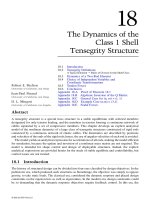
The artist Kenneth Snelson

1

(Figure 17.1) built the first tensegrity structure and his artwork was
the inspiration for the first author’s interest in tensegrity. Buckminster Fuller

2

coined the word

“tensegrity” from two words: “tension” and “integrity.”

17.1.1 The Benefits of Tensegrity

A large amount of literature on the geometry, artform, and architectural appeal of tensegrity
structures exists, but there is little on the dynamics and mechanics of these structures.

2-19

Form-
finding results for simple symmetric structures appear

10,20-24

and show an array of stable tensegrity
units is connected to yield a large stable system, which can be deployable.

14

Tensegrity structures
for civil engineering purposes have been built and described.

25-27

Several reasons are given below
why tensegrity structures should receive new attention from mathematicians and engineers, even
though the concepts are 50 years old.

17.1.1.1 Tension Stabilizes

A compressive member loses stiffness as it is loaded, whereas a tensile member gains stiffness as
it is loaded. Stiffness is lost in two ways in a compressive member. In the absence of any bending
moments in the axially loaded members, the forces act exactly through the mass center, the material
spreads, increasing the diameter of the center cross section; whereas the tensile member reduces
its cross-section under load. In the presence of bending moments due to offsets in the line of force
application and the center of mass, the bar becomes softer due to the bending motion. For most
materials, the tensile strength of a longitudinal member is larger than its buckling (compressive)

8596Ch17Frame Page 316 Friday, November 9, 2001 6:33 PM
© 2002 by CRC Press LLC

strength. (Obviously, sand, masonary, and unreinforced concrete are exceptions to this rule.) Hence,
a large stiffness-to-mass ratio can be achieved by increasing the use of tensile members.

17.1.1.2 Tensegrity Structures are Efficient

It has been known since the middle of the 20th century that continua cannot explain the strength of
materials. The geometry of material layout is critical to strength at all scales, from nanoscale biological
systems to megascale civil structures. Traditionally, humans have conceived and built structures in
rectilinear fashion. Civil structures tend to be made with orthogonal beams, plates, and columns.
Orthogonal members are also used in aircraft wings with longerons and spars. However, evidence
suggests that this “orthogonal” architecture does not usually yield the minimal mass design for a given
set of stiffness properties.

28

Bendsoe and Kikuchi,

29

Jarre,

30

and others have shown that the optimal
distribution of mass for specific stiffness objectives tends to be neither a solid mass of material with
a fixed external geometry, nor material laid out in orthogonal components. Material is needed only in
the essential load paths, not the orthogonal paths of traditional manmade structures.

Tensegrity structures

use longitudinal members arranged in very unusual (and nonorthogonal) patterns to achieve strength
with small mass. Another way in which tensegrity systems become mass efficient is with self-similar
constructions replacing one tensegrity member by yet another tensegrity structure.

17.1.1.3 Tensegrity Structures are Deployable

Materials of high strength tend to have a very limited displacement capability. Such piezoelectric
materials are capable of only a small displacement and “smart” structures using sensors and
actuators have only a small displacement capability. Because the compressive members of tensegrity
structures are either disjoint or connected with ball joints, large displacement, deployability, and
stowage in a compact volume will be immediate virtues of tensegrity structures.

8,11

This feature
offers operational and portability advantages. A portable bridge, or a power transmission tower
made as a tensegrity structure could be manufactured in the factory, stowed on a truck or helicopter
in a small volume, transported to the construction site, and deployed using only winches for erection
through cable tension. Erectable temporary shelters could be manufactured, transported, and

deployed in a similar manner. Deployable structures in space (complex mechanical structures
combined with active control technology) can save launch costs by reducing the mass required, or
by eliminating the requirement for assembly by humans.

FIGURE 17.1

Snelson’s tensegrity structure. (From Connelly, R. and Beck, A.,

American Scientist,

86(2), 143,
1998. Kenneth Snelson, Needle Tower 11, 1969, Kröller Müller Museum. With permission.)

8596Ch17Frame Page 317 Friday, November 9, 2001 6:33 PM
© 2002 by CRC Press LLC

17.1.1.4 Tensegrity Structures are Easily Tunable

The same deployment technique can also make small adjustments for fine tuning of the loaded
structures, or adjustment of a damaged structure. Structures that are designed to allow tuning will be
an important feature of next generation mechanical structures, including civil engineering structures.

17.1.1.5 Tensegrity Structures Can be More Reliably Modeled

All members of a tensegrity structure are axially loaded. Perhaps the most promising scientific
feature of tensegrity structures is that while the

global

structure bends with external static loads,

none of the

individual

members of the tensegrity structure experience bending moments. (In this
chapter, we design all compressive members to experience loads well below their Euler buckling
loads.) Generally, members that experience deformation in two or three dimensions are much harder
to model than members that experience deformation in only one dimension. The Euler buckling
load of a compressive member is from a bending instability calculation, and it is known in practice
to be very unreliable. That is, the actual buckling load measured from the test data has a larger
variation and is not as predictable as the tensile strength. Hence, increased use of tensile members
is expected to yield more robust models and more efficient structures. More reliable models can
be expected for axially loaded members compared to models for members in bending.

31

17.1.1.6 Tensegrity Structures Facilitate High Precision Control

Structures that can be more precisely modeled can be more precisely controlled. Hence, tensegrity
structures might open the door to quantum leaps in the precision of controlled structures. The
architecture (geometry) dictates the mathematical properties and, hence, these mathematical results
easily scale from the nanoscale to the megascale, from applications in microsurgery to antennas,
to aircraft wings, and to robotic manipulators.

17.1.1.7 Tensegrity is a Paradigm that Promotes the Integration of Structure
and Control Disciplines

A given tensile or compressive member of a tensegrity structure can serve multiple functions. It
can simultaneously be a load-carrying member of the structure, a sensor (measuring tension or
length), an actuator (such as nickel-titanium wire), a thermal insulator, or an electrical conductor.

In other words, by proper choice of materials and geometry, a grand challenge awaits the tensegrity
designer: How to control the electrical, thermal, and mechanical energy in a material or structure?
For example, smart tensegrity wings could use shape control to maneuver the aircraft or to optimize
the air foil as a function of flight condition, without the use of hinged surfaces. Tensegrity structures
provide a promising paradigm for integrating structure and control design.

17.1.1.8 Tensegrity Structures are Motivated from Biology

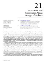
Figure 17.2 shows a rendition of a spider fiber, where amino acids of two types have formed hard

β−

pleated sheets that can take compression, and thin strands that take tension.

32,33

The

β−

pleated
sheets are discontinuous and the tension members form a continuous network. Hence, the nano-
structure of the spider fiber is a tensegrity structure. Nature’s endorsement of tensegrity structures
warrants our attention because per unit mass, spider fiber is the strongest natural fiber.
Articles by Ingber

7,34,35

argue that tensegrity is the fundamental building architecture of life. His
observations come from experiments in cell biology, where prestressed truss structures of the

tensegrity type have been observed in cells. It is encouraging to see the similarities in structural
building blocks over a wide range of scales. If tensegrity is nature’s preferred building architecture,
modern analytical and computational capabilities of tensegrity could make the same incredible
efficiency possessed by natural systems transferrable to manmade systems, from the nano- to the
megascale. This is a grand design challenge, to develop scientific procedures to create smart
tensegrity structures that can regulate the flow of thermal, mechanical, and electrical energy in a
material system by proper choice of materials, geometry, and controls. This chapter contributes to
this cause by exploring the mechanical properties of simple tensegrity structures.

8596Ch17Frame Page 318 Friday, November 9, 2001 6:33 PM
© 2002 by CRC Press LLC

The remainder of the introduction describes the main results of this chapter. We start with formal
definitions and then turn to results.

17.1.2 Definitions and Examples

This is an introduction to the mechanics of a class of prestressed structural systems that are
composed only of axially loaded members. We need a couple of definitions to describe tensegrity
scientifically.

Definition 17.1

We say that the geometry of a material system is in a stable equilibrium if all
particles in the material system return to this geometry, as time goes to infinity, starting from any
initial position arbitrarily close to this geometry.

In general, a variety of boundary conditions may be imposed, to distinguish, for example, between
bridges and space structures. But, for the purposes of this chapter we characterize only the material
system with free–free boundary conditions, as for a space structure. We will herein characterize

the bars as rigid bodies and the strings as one-dimensional elastic bodies. Hence, a material system
is in equilibrium if the nodal points of the bars in the system are in equilibrium.

Definition 17.2

A

Class k tensegrity structure

is a stable equilibrium of axially loaded elements,
with a maximum of k compressive members connected at the node(s).

Fact 17.1

Class k tensegrity structures

must have tension members

.
Fact 17.1 follows from the requirement to have a stable equilibrium.

Fact 17.2

Kenneth Snelson’s structures of which

Figure

17.1 is an example are all

Class 1

tensegrity structures,

using Definition 17.1. Buckminster Fuller coined the word tensegrity to imply
a connected set of tension members and a disconnected set of compression members. This fits our
“Class 1” definition.

A Class 1 tensegrity structure has a connected network of members in tension, while the network
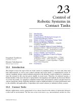
of compressive members is disconnected. To illustrate these various definitions, Figure 17.3(a)

FIGURE 17.2

Structure of the Spider Fiber. (From Termonia, Y.,

Macromolecules

, 27, 7378–7381, 1994.
Reprinted with permission from the American Chemical Society.)
amorphous
chain
β-pleated sheet
entanglement
hydrogen bond
y
z
x
6nm

8596Ch17Frame Page 319 Friday, November 9, 2001 6:33 PM
© 2002 by CRC Press LLC

illustrates the simplest tensegrity structure, composed of one bar and one string in tension. Thin
lines are strings and shaded bars are compressive members. Figure 17.3(b) describes the next
simplest arrangement, with two bars. Figure 17.3(c) is a Class 2 tensegrity structure because two
bars are connected at the nodes. Figure 17.3(c) represents a Class 2 tensegrity in the plane. However,
as a three-dimensional structure, it is not a tensegrity structure because the equilibrium is unstable
(the tensegrity definition requires a stable equilibrium).
From these definitions, the existence of a tensegrity structure having a specified geometry reduces
to the question of whether there exist finite tensions that can be applied to the tensile members to
hold the system in that geometry, in a stable equilibrium.
We have illustrated that the geometry of the nodal points and the connections cannot be arbitrarily
specified. The role that geometry plays in the mechanical properties of tensegrity structures is the
focus of this chapter.
The planar tensegrity examples shown follow a naming convention that describes the number of
compressive members and tension members. The number of compressive members is associated
with the letter C, while the number of tensile members is associated with T. For example, a structure
that contains two compressive members and four tension members is called a

C

2

T

4 tensegrity.

17.1.3 The Analyzed Structures

The basic examples we analyzed are the structures shown in Figure 17.4, where thin lines are the
strings and the thick lines are bars. Also, we analyzed various structures built from these basic
structural units. Each structure was analyzed under several types of loading. In particular, the top

and bottom loads indicated on the

C

2

T

4 structure point in opposite directions, thereby resulting in
bending. We also analyzed a

C

2

T

4 structure with top and bottom loads pointing in the same
direction, that is, a compressive situation. The

C

4

T

2 structure of Figure 17.4(b) reduces to a

C

4

T

1
structure when the horizontal string is absent. The mass and stiffness properties of such structures
will be of interest under compressive loads,

F

, as shown. The 3-bar SVD (defined in 17.4.1) was
studied under two types of loading: axial and lateral. Axial loading is compressive while lateral
loading results in bending.

17.1.4 Main Results on Tensegrity Stiffness

A reasonable test of any tensegrity structure is to apply several forces each of magnitude

F

at
several places and plot how some measure of its shape changes. We call the plot of vs.

F

a stiffness profile of the structure. The chapter analyzes stiffness profiles of a variety of tensegrity
structures. We paid special attention to the role of pretension set in the strings of the tensegrity.
While we have not done an exhaustive study, there are properties common to these examples which
we now describe. How well these properties extend to all tensegrity structures remains to be seen.

FIGURE 17.3

Tensegrity structures.
dF dshape

8596Ch17Frame Page 320 Friday, November 9, 2001 6:33 PM
© 2002 by CRC Press LLC

However, laying out the principles here is an essential first step to discovering those universal
properties that do exist.
The following example with masses and springs prepares us for two basic principles which we
have observed in the tensegrity paradigm.

17.1.4.1 Basic Principle 1: Robustness from Pretension

As a parable to illustrate this phenomenon, we resort to the simple example of a mass attached to
two bungy cords. (See Figure 17.5.)
Here

K

L

,

K

R

are the spring constants,

F

is an external force pushing right on the mass, and

t

L

,

t

R

are tensions in the bungy cords when

F

= 0. The bungy cords have the property that when they
are shorter than their rest length they become inactive. If we set any positive pretensions

t

L

,

t

R

,
there is a corresponding equilibrium configuration, and we shall be concerned with how the shape
of this configuration changes as force

F

is applied. Shape is a peculiar word to use here when we
mean position of the mass, but it forshadows discussions about very general tensegrity structures.
The effect of the stiffness of the structure is seen in Figure 17.6.

FIGURE 17.4

Tensegrities studied in this chapter (not to scale), (a)

C

2

T

4 bending loads (left) and compressive
loads (right), (b)

C

4

T

2, and (c) 3-bar SVD axial loads (left) and lateral loads (right).

FIGURE 17.5

Mass–spring system.
(a)
(b)
(c)
8596Ch17Frame Page 321 Friday, November 9, 2001 6:33 PM
© 2002 by CRC Press LLC
There are two key quantities in this graph which we see repeatedly in tensegrity structures. The
first is the critical value F
1
where the stiffness drops. It is easy to see that F
1
equals the value of
F at which the right cord goes slack. Thus, F
1
increases with the pretension in the right cord. The
second key parameter in this figure is the size of the jump as measured by the ratio
When r = 1, the stiffness plot is a straight horizontal line with no discontinuity. Therefore, the
amount of pretension affects the value of F
1
, but has no influence on the stiffness. One can also
notice that increasing the value of r increases the size of the jump. What determines the size of r
is just the ratio κ of the spring constants , since r = 1 + κ, indeed r is an increasing
function of κ
r ≅ ∞ if κ ≅ ∞.
Of course, pretension is impossible if K

R
= 0. Pretension increases F
1
and, hence, allows us to stay
in the high stiffness regime given by S
tens
, over a larger range of applied external force F.
17.1.4.2 Robustness from Pretension Principle for Tensegrity Structures
Pretension is known in the structures community as a method of increasing the load-bearing capacity
of a structure through the use of strings that are stretched to a desired tension. This allows the structure
to support greater loads without as much deflection as compared to a structure without any pretension.
For a tensegrity structure, the role of pretension is monumental. For example, in the analysis of
the planar tensegrity structure, the slackening of a string results in dramatic nonlinear changes in
the bending rigidity. Increasing the pretension allows for greater bending loads to be carried by
the structure while still exhibiting near constant bending rigidity. In other words, the slackening of
a string occurs for a larger external load. We can loosely describe this as a robustness property, in
that the structure can be designed with a certain pretension to accomodate uncertainties in the
loading (bending) environment. Not only does pretension have a consequence for these mechanical
properties, but also for the so-called prestressable problem, which is left for the statics problem.
The prestressable problem involves finding a geometry which can sustain its shape without external
forces being applied and with all strings in tension.
12,20
17.1.4.2.1 Tensegrity Structures in Bending
What we find is that bending stiffness profiles for all examples we study have levels S
tens
when all
strings are in tension, S
slack1
when one string is slack, and then other levels as other strings go slack
or as strong forces push the structure into radically different shapes (see Figure 17.7). These very

high force regimes can be very complicated and so we do not analyze them. Loose motivation for
FIGURE 17.6 Mass–spring system stiffness profile.
r
S
S
tens
slack
:=
κ:= KK
RL
8596Ch17Frame Page 322 Friday, November 9, 2001 6:33 PM
© 2002 by CRC Press LLC
the form of a bending stiffness profile curve was given in the mass and two bungy cord example,
in which case we had two stiffness levels.
One can imagine a more complicated tensegrity geometry that will possibly yield many stiffness
levels. This intuition arises from the possibility that multiple strings can become slack depending
on the directions and magnitudes of the loading environment. One hypothetical situation is shown
in Figure 17.7 where three levels are obtained. All tensegrity examples in the chapter have bending
stiffness profiles of this form, at least until the force F radically distorts the figure. The specific
profile is heavily influenced by the geometry of the tensegrity structure as well as of the stiffness
of the strings, K
string
, and bars, K
bar
. In particular, the ratio
is an informative parameter.
General properties common to our bending examples are
1. When no string is slack, the geometry of a tensegrity and the materials used have much more
effect on its stiffness than the amount of pretension in its strings.
2. As long as all strings are in tension (that is, F < F

1
), stiffness has little dependence on F or
on the amount of pretension in the strings.
3. A larger pretension in the strings produces a larger F
1
.
4. As F exceeds F
1
the stiffness quickly drops.
5. The ratio
is an increasing function of K. Moreover, r
1
→ ∞ as K → ∞ (if the bars are flabby, the
structure is flabby once a string goes slack). Similar parameters, r
2
, can be defined for each
change of stiffness.
Examples in this chapter that substantiate these principles are the stiffness profile of C2T4 under
bending loads as shown in Figure 17.12. Also, the laterally loaded 3-bar SVD tensegrity shows the
same behavior with respect to the above principles, Figure 17.54 and Figure 17.55.
17.1.4.2.2 Tensegrity Structures in Compression
For compressive loads, the relationships between stiffness, pretension, and force do not always
obey the simple principles listed above. In fact, we see three qualitatively different stiffness profiles
in our compression loading studies. We now summarize these three behavior patterns.
FIGURE 17.7 Gedanken stiffness profile.
K
K
K
:=
string

bar
r
S
S
1
:=
tens
slack
8596Ch17Frame Page 323 Friday, November 9, 2001 6:33 PM
© 2002 by CRC Press LLC
The C2T4 planar tensegrity exhibits the pretension robustness properties of Principles I, II, III,
as shown in Figure 17.6. The pretension tends to prevent slack strings.
The C4T2 structure has a stiffness profile of the form in Figure 17.8. Only in the C4T1 and C4T2
examples does stiffness immediately start to fall as we begin to apply a load.
The axially loaded 3-bar-SVD, the stiffness profile even for small forces, is seriously affected
by the amount of pretension in the structure. Rather than stiffness being constant for F < F
1
as is
the case with bending, we see in Figure 17.9 that stiffness increases with F for small and moderate
forces. The qualitative form of the stiffness profile is shown in Figure 17.9. We have not system-
atically analyzed the role of the stiffness ratio K in compression situations.
17.1.4.2.3 Summary
Except for the C4T2 compression situation, when a load is applied to a tensegrity structure the
stiffness is essentially constant as the loading force increases unless a string goes slack.
17.1.4.3 Basic Principle 2: Changing Shape with Small Control Energy
We begin our discussion not with a tensegrity structure, but with an analogy. Imagine, as in
Figure 17.10, that the rigid boundary conditions of Figure 17.5 become frictionless pulleys. Suppose
we are able to actuate the pulleys and we wish to move the mass to the right, we can turn each
pulley clockwise. The pretension can be large and yet very small control torques are needed to
change the position of the nodal mass.

FIGURE 17.8 Stiffness profile for C4T2 in compression.
FIGURE 17.9 Stiffness profile of 3-bar SVD in compression.
FIGURE 17.10 Mass–spring control system.
8596Ch17Frame Page 324 Friday, November 9, 2001 6:33 PM
© 2002 by CRC Press LLC
Tensegrity structures, even very complicated ones, can be actuated by placing pulleys at the
nodes (ends of bars) and running the end of each string through a pulley. Thus, we think of two
pulleys being associated with each string and the rotation of the pulleys can be used to shorten or
loosen the string. The mass–spring example foreshadows the fact that even in tensegrity structures,
shape changes (moving nodes changes the shape) can be achieved with little change in the potential
energy of the system.
17.1.5 Mass vs. Strength
The chapter also considers the issue of the strength vs. mass of tensegrity structures. We find our
planar examples to be very informative. We shall consider two types of strength. They are the size
of the bending forces and the size of compressive forces required to break the object.
First, in 17.2 we study the ratio of bending strength to mass. We compare this for our C2T4 unit
to a solid rectangular beam of the same mass. As expected, reasonably constructed C2T4 units will
be stronger. We do this comparison to a rectangular beam by way of illustrating the mass vs.
strength question, because a thorough study would compare tensegrity structures to various kinds
of trusses and would require a very long chapter.
We analyze compression stiffness of the C2T4 tensegrity. The C2T4 has worse strength under
compression than a solid rectangular bar. We analyze the compression stiffness of C4T2 and
C4T1 structures and use self-similar concepts to reduce mass, while constraining stiffness to a
desired value. The C4T1 structure has a better compression strength-to-mass ratio than a solid
bar when δ < 29°. The C4T1, while strong (not easily broken), may not have an extremely high
stiffness.
17.1.5.1 A 2D Beam Composed of Tensegrity Units
After analyzing one C2T4 tensegrity unit, we lay n of them side by side to form a beam. We derive
in 17.2.3 that the Euler buckling formula for a beam adapts directly to this case. From this we
conclude that the strength of the beam under compression is determined primarily by the bending

rigidity (EI)
n
of each of its units. In principle, one can build beams with arbitrarily great bending
strength. In practice this requires more study. Thus, the favorable bending properties found for
C2T4 bode well for beams made with tensegrity units.
17.1.5.2 A 2D Tensegrity Column
In 17.3 we take the C4T2 structure in Figure 17.4(b) and replace each bar with a smaller C4T2
structure, then we replace each bar of this new structure with a yet smaller C4T2 structure. In
principle, such a self-similar construction can be repeated to any level. Assuming that the strings
do not fail and have significantly less mass than the bars, we find that the compression strength
increases without bound if we keep the mass of the total bars constant. This completely ignores
the geometrical fact that as we go to finer and finer levels in the fractal construction, the bars
increasingly overlap. Thus, at least in theory, we have a class of tensegrity structures with
unlimited compression strength to mass ratio. Further issues of robustness to lateral and bending
forces would have to be investigated to insure practicality of such structures. However, our
dramatic findings based on a pure compression analysis are intriguing. The self-similar concept
can be extended to the third dimension in order to design a realistic structure that could be
implemented in a column.
The chapter is arranged as follows: Section 17.2 analyzes a very simple planar tensegrity structure
to show an efficient structure in bending; Section 17.3 analyzes a planar tensegrity structure efficient
in compression; Section 17.4 defines a shell class of tensegrity structures and examines several
members of this class; Section 17.5 offers conclusions and future work. The appendices explain
nonlinear and linear analysis of planar tensegrity.
8596Ch17Frame Page 325 Friday, November 9, 2001 6:33 PM
© 2002 by CRC Press LLC
17.2 Planar Tensegrity Structures Efficient in Bending
In this section, we examine the bending rigidity of a single tensegrity unit, a planar tensegrity
model under pure bending as shown in Figure 17.11, where thin lines are the four strings and the
two thick lines are bars. Because the structure in Figure 17.11 has two compressive and four tensile
members, we refer to it as a C2T4 structure.

17.2.1 Bending Rigidity of a Single Tensegrity Unit
To arrive at a definition of bending stiffness suitable to C2T4, note that the moment M acting on
the section is given by
M = FL
bar
sin δ, (17.1)
where F is the magnitude of the external force, L
bar
is the length of the bar, and δ is the angle that
the bars make with strings in the deformed state, as shown in Figure 17.11.
In Figure 17.11, ρ is the radius of curvature of the tensegrity unit under bending deformation.
It can be shown from Figure 17.11 that
(17.2)
The bending rigidity is defined by EI = Mρ. Hence,
(17.3)
where EI is the equivalent bending rigidity of the planar one-stage tensegrity unit and u is the nodal
displacement. The evaluation of the bending rigidity of the planar unit requires the evaluation of
u, which will follow under various hypotheses. The bending rigidity will later be obtained by
substituting u in (17.3).
FIGURE 17.11 Planar one-stage tensegrity unit under pure bending.
ρδδ δθ=






=
L
u

uL
bar
bar
2
1
2
2
cos sin
1
sin tan .,
EI FL FL
L
u
bar bar
bar
==






sin sin cos
1
2
δρ δ δ
2
2
.
8596Ch17Frame Page 326 Friday, November 9, 2001 6:33 PM

© 2002 by CRC Press LLC
17.2.1.1 Effective Bending Rigidity with Pretension
In the absence of external forces f, let A
0
be the matrix defined in Appendix 17.A in terms of the
initial prestressed geometry, and let t
0
be the initial pretension applied on the members of the
tensegrity. Then,
(17.4)
For a nontrivial solution of Equation (17.4), A
0
must have a right null space. Furthermore, the
elements of t
0
obtained by solving Equation (17.4) must be such that the strings are always in
tension, where t
0-strings
≥ 0 will be used to denote that each element of the vector is nonnegative.
For this particular example of planar tensegrity, the null space of A
0
is only one dimensional. t
0
always exists, satisfying (17.4), and t
0
can be scaled by any arbitrary positive scalar multiplier.
However, the requirement of a stable equilibrium in the tensegrity definition places one additional
constraint to the conditions (17.4); the geometry from which A
0
is constructed must be a stable

equilibrium.
In the following discussions, E
s
, (EA)
s
, and A
s
denote the Young’s modulus of elasticity, the axial
rigidity and the cross-sectional area of the strings, respectively, whereas E
b
, (EA)
b
, and A
b
, denote
those of the bars, respectively. (EI)
b
denotes the bending rigidity of the bars.
The equations of the static equilibrium and the bending rigidity of the tensegrity unit are nonlinear
functions of the geometry δ, the pretension t
0
, the external force F, and the stiffnesses of the strings
and bars. In this case, the nodal displacement u is obtained by solving nonlinear equations of the static
equilibrium (see Appendix 17.A for the underlying assumptions and for a detailed derivation)
A (u) KA (u)
T
u = F – A (u)t
0
(17.5)
Also, t

0
is the pretension applied in the strings, K is a diagonal matrix containing axial stiffness of
each member, i.e., K
ii
= (EA)
i
/L
i
, where L
i
is the length of the i-th member; u represents small nodal
displacements in the neighborhood of equilibrium caused by small increments in the external forces.
The standard Newton–Raphson method is applied to solve (17.5) at each incremental load step F
k
=
F
k-1
+ ∆F. Matrix A(u
k
) is updated at each iteration until a convergent solution for u
k
is found.
Figure 17.12 depicts EI as a function of the angle δ, pretension of the top string, and the rigidity
ratio K which is defined as the ratio of the axial rigidity of the strings to the axial rigidity of the
bars, i.e., K = (EA)
s
/(EA)
b
. The pretension is measured as a function of the prestrain in the top
string Σ

0
. In obtaining Figure 17.12, the bars were assumed to be equal in diameter and the strings
were also assumed to be of equal diameter. Both the bars as well as the strings were assumed to
be made of steel for which Young’s modulus of elasticity E was taken to be 2.06 × 10
11
N/m
2
, and
the yield strength of the steel σ
y
was taken to be 6.90 × 10
8
N/m
2
. In Figure 17.12, EI is plotted
against the ratio of the external load F to the yield force of the string. The yield force of the string
is defined as the force that causes the strings to reach the elastic limit. The yield force for the
strings is computed as
Yield force of string = σ
y
A
s
,
where σ
y
is the yield strength and A
s
is the cross-sectional area of the string. The external force F
was gradually increased until at least one of the strings yielded.
The following conclusions can be drawn from Figure 17.12:

1. Figure 17.12(a) suggests that the bending rigidity EI of a tensegrity unit with all taut strings
increases with an increase in the angle δ, up to a maximum at δ = 90°.
2. Maximum bending rigidity EI is obtained when none of the strings is slack, and the EI is
approximately constant for any external force until one of the strings go slack.

At 0 t t t t
00
== ≥, [ ], .
0
00
-

0
0
T
bars
strings strings
8596Ch17Frame Page 327 Friday, November 9, 2001 6:33 PM
© 2002 by CRC Press LLC
3. Figure 17.12(b) shows that the pretension does not have much effect on the magnitude of
EI of a planar tensegrity unit. However, pretension does play a remarkable role in preventing
the string from going slack which, in turn, increases the range of the constant EI against
external loading. This provides robustness of EI predictions against uncertain external forces.
This feature provides robustness against uncertainties in external forces.
4. In Figure 17.12(c) we chose structures having the same geometry and the same total stiffness,
but different K, where K is the ratio of the axial rigidity of the bars to the axial rigidity of
the strings. We then see that K has little influence on EI as long as none of the strings are
slack. However, the bending rigidity of the tensegrity unit with slack string influenced K,
with maximum EI occurring at K = 0 (rigid bars).
It was also observed that as the angle δ is increased or as the stiffness of the bar is decreased,

the force-sharing mechanism of the members of the tensegrity unit changes quite noticeably. This
phenomena is seen only in the case when the top string is slack. For example, for K = 1/9 and ε
0
=
0.05%, for small values of δ, the major portion of the external force is carried by the bottom string,
whereas after some value of δ (greater than 45°), the major portion of the external force is carried
by the vertical side strings rather than the bottom string. In such cases, the vertical side strings
FIGURE 17.12 Bending rigidity EI of the planar tensegrity unit for (a) different initial angle δ with rigidity ratio
K = 1/9 and prestrain in the top string ε
0
= 0.05%, (b) different ε
0
with K = 1/9, (c) different K with δ = 60° and ε
0
=
0.05%. L
bar
for all cases is 0.25 m.
(a) (b) (c)
8596Ch17Frame Page 328 Friday, November 9, 2001 6:33 PM
© 2002 by CRC Press LLC
could reach their elastic limit prior to the bottom string. Similar phenomena were also observed
for a case of K = 100, δ = 60°, and ε
0
= 0.05%. In such cases, as shown in Figure 17.12(a) for δ =
70° and δ = 75°, the EI drops drastically once the top string goes slack. Figure 17.13 summarizes
the conclusions on bending rigidity, where the arrows indicate increasing directions of δ, t
0
, or K.
Note that when t

0
is the pretension applied to the top string, the pretension in the vertical side
strings is equal to t
0
/tan δ. The cases of δ > 80° were not computed, but it is clear that the bending
rigidity is a step function as δ approaches 90°, with EI constant until the top string becomes slack,
then the EI goes to zero as the external load increases further.
17.2.1.2 Bending Rigidity of the Planar Tensegrity for the Rigid Bar Case (K = 0)
The previous section briefly described the basis of the calculations for Figure 17.11. The following
sections consider the special case K = 0 to show more analytical insight. The nonslack case describes
the structure when all strings exert force. The slack case describes the structure when string 3 exerts
zero force, due to the deformation of the structure. Therefore, the force in string 3 must be computed
to determine when to switch between the slack and nonslack equations.
17.2.1.2.1 Some Relations from Geometry and Statics
Nonslack Case: Summing forces at each node we obtain the equilibrium conditions
ƒ
c
cos δ = F + t
3
– t
2
sin θ (17.6)
ƒ
c
cos δ = t
1
+ t
2
sin θ – F (17.7)
ƒ

c
sin δ = t
2
cos θ, (17.8)
where ƒ
c
is the compressive load in a bar, F is the external load applied to the structure, and t
i
is
the force exerted by string i defined as
t
i
= k
i
(l
i
– l
i0
). (17.9)
The following relations are defined from the geometry of Figure 17.11:
l
1
= L
bar
cos δ + L
bar
tan θ sin δ
l
2
= L

bar
sin δ sec θ
l
3
= L
bar
cos δ – L
bar
sin δ tan θ
h = L
bar
sin δ, (17.10)
FIGURE 17.13 Trends relating geometry δ, prestress t
0
, and material K.
8596Ch17Frame Page 329 Friday, November 9, 2001 6:33 PM
© 2002 by CRC Press LLC
where l
i
denote the geometric length of the strings. We will find the relation between δ and θ by
eliminating f
c
and F from (17.6)–(17.8)
(17.11)
Substitution of relations (17.10) and (17.9) into (17.11) yields
(17.12)
If k
i
= k, then (17.12) simplifies to
(17.13)

Slack Case: In order to find a relation between δ and θ for the slack case when t
3
has zero
tension, we use (17.12) and set k
3
to zero. With the simplification that we use the same material
properties, we obtain
0 = L
bar
tan θ sin δ tan δ + 2l
20
cos θ – l
10
tan δ – L
bar
sin δ. (17.14)
This relationship between δ and θ will be used in (17.22) to describe bending rigidity.
17.2.1.2.2 Bending Rigidity Equations
The bending rigidity is defined in (17.3) in terms of ρ and F. Now we will solve the geometric and
static equations for ρ and F in terms of the parameters θ, δ of the structure. For the nonslack case,
we will use (17.13) to get an analytical formula for the EI. For the slack case, we do not have an
analytical formula. Hence, this must be done numerically.
From geometry, we can obtain ρ,
Solving for ρ we obtain
(17.15)
Nonslack Case: In the nonslack case, we now apply the relation in (17.13) to simplify (17.15)
(17.16)
cos tan .θδ=
+tt
t

13
2
2
cos
( cos tan sin ) ( cos tan sin )
( sin sec )
tan
+
.θ
δθδ δθδ
δθ
δ=
−+ − −
−
kL L l kL L l
kL l
bar bar bar bar
bar
110330
220
2
tan δθβθ=
+
2
20
10 30
l
ll
cos = cos .
tan

()
θ
ρ
=
+
l
h
1
2
2
.
ρ
θ
δθδ
θ
δ
δ
θ
=−
+
−
=
l
h
LL L
L
bar bar bar
bar
1
22

22
2
tan
cos tan sin
tan
sin
cos
tan
.

=

ρ
θβ θ
=
+
L
bar
2
1
1
22
tan cos
.
8596Ch17Frame Page 330 Friday, November 9, 2001 6:33 PM
© 2002 by CRC Press LLC
From (17.6)–(17.8) we can solve for the equilibrium external F
– k
3
L

bar
cos δ + k
3
L
bar
sin δ tan θ + k
3
l
30
). (17.17)
Again, using (17.13) and k
i
= k, Equation (17.17) simplifies to
(17.18)
We can substitute (17.18) and (17.16) into (17.3)
(17.19)
and we obtain the bending rigidity of the planar structure with no slack strings present. The
expression for string length l
3
in the nonslack case reduces to
(17.20)
This expression can be used to determine the angle which causes l
3
to become slack.
Slack Case: Similarly, for the case when string 3 goes slack, we set k
3
= 0 and k
i
= k in (17.17),
which yield simply

(17.21)
and
(17.22)
See Figure 17.12(c) for a plot of EI for the K = 0 (rigid bar) case.
17.2.1.2.3 Constants and Conversions
All plots shown are generated with the following data which can then be converted as follows if
necessary.
Ftt t
kL kL kl
kL kl
bar bar
bar
=+ −
=+ −
+−
1
2
2
1
2
22
12 3
11 110
2220
( sin )
( cos tan sin
sin tan sin
θ
δθδ
δθ θ

F
kL
k
ll l
bar
=
+
−−
2
1
2
2
22
10 30 20
βθ
βθ
θ
sin
cos
sin ( + ).

El
LkL
k
ll l
bar bar
=
+
+
−−







22
22
22
10 30 20
21
2
1
2
2
βθ
βθθ
βθ
βθ
θ
cos
( cos ) (sin )
sin
cos
sin , ( + )


lL
bar
3

22
=
1 + cos
1−β θ
βθ

sin
.
Ftt
kL kL kl kl
slack
bar bar
= ( + )
= (
1
2
2
1
2
32
12
10 20
sin
cos tan sin sin )
θ
δθδ θ+−−
EI
L
kL kL kl kl
slack

bar
bar bar
=

(
2
10 20
4
32
sin cos
tan
cos tan sin sin ).
δδ
θ
δθδ θ+−−
8596Ch17Frame Page 331 Friday, November 9, 2001 6:33 PM
© 2002 by CRC Press LLC
Young’s Modulus, E = 2.06 × 10
11
N/m
2
Yield Stress, σ = 6.9 × 10
8
N/m
2
Diameter of Tendons = 1 mm
Cross-Sectional Area of Tendon = 7.8540 × 10
–7
m
2

Length of Bar, L
bar
= .25 m
Prestress = e
0
Initial Angle = δ
0
The spring constant of a string is
(17.23)
The following equation can be used to compute the equivalent rest length given some measure
of prestress t
0
t
0
= (EA)
s
e
0
= k(l – l
0
)
. (17.24)
17.2.1.3 Effective Bending Rigidity with Slack String (K > 0)
As noted earlier, the tensegrity unit is a statically indeterminate structure (meaning that matrix A
is not full column rank) as long as the strings remain taut during the application of the external
load. However, as soon as one of the strings goes slack, the tensegrity unit becomes statically
determinate. In the following, an expression for bending rigidity of the tensegrity unit with an
initially slack top string is derived. Even in the case of a statically determinate tensegrity unit with
slack string, the problem is still a large displacement and nonlinear problem. However, a linear
solution, valid for small displacements only, resulting in a quite simple and analytical form can be

found. Based on the assumptions of small displacements, an analytical expression for EI of the
tensegrity unit with slack top string has been derived in Appendix 17.B and is given below.
(17.25)
The EI obtained from nonlinear analysis, i.e., from (17.3) together with (17.5), is compared with
the EI obtained from linear analysis, i.e., from (17.25), and is shown in Figure 17.14. Figure 17.14
shows that the linear analysis provides a lower bound to the actual bending rigidity. The linear
estimation of EI, i.e., (17.25), is plotted in Figure 17.15 as a function of the initial angle δ for
different values of the stiffness ratio K. Both bars and the strings are assumed to be made of steel,
as before. It is seen in Figure 17.15 that the EI of the tensegrity unit with slack top string attains
a maximum value for some value of δ. The decrease of EI (after the maximum) is due to the change
in the force sharing mechanism of the members of the tensegrity unit, as discussed earlier. For
small values of δ, the major portion of the external force is carried by the bottom string, whereas
for larger values of δ, the vertical side strings start to share the external force. As δ is further

k
EA
L
bar
=
cos( )
.
δ
0
lL
EAe
k
bar
00
0
=

cos( )δ−
EI
LEA
K
bar
s
≈
++
1
22
2
23
33
( ) sin cos
(sin cos )
.
δδ
δδ
8596Ch17Frame Page 332 Friday, November 9, 2001 6:33 PM
© 2002 by CRC Press LLC
increased, the major portion of the external force is carried by the vertical side strings rather than
the bottom string. This explains the decrease in EI with the increase in δ after some values of δ
for which EI is maximum.
The locus of the maximum EI is also shown in Figure 17.15. The maximum value of EI and the
δ for which EI is maximum depend on the relative stiffness of the string and the bars, i.e., they
depend on K. From Figure 17.15 note that the maximum EI is obtained when the bars are much
FIGURE 17.14 Comparison of EI from nonlinear analysis with the EI from linear analysis with slack top string
(L
bar
= 0.25 m, δ = 60° and K = 1/9).

FIGURE 17.15 EI with slack top string with respect to the angle δ for L
bar
= 0.25m.
8596Ch17Frame Page 333 Friday, November 9, 2001 6:33 PM
© 2002 by CRC Press LLC
stiffer than the strings. EI is maximum when the bars are perfectly rigid, i.e., K → 0. It is seen in
Figure 17.15 and can also be shown analytically from (17.25) that for the case of bars much stiffer
than the strings, K → 0, the maximum EI of the tensegrity unit with slack top string is obtained
when δ = 45°. In constrast, note from Figure 17.12(a) that when no strings are slack, the maximum
bending rigidity occurs with δ = 90°.
17.2.2 Mass Efficiency of the C2T4 Class 1 Tensegrity in Bending
This section demonstrates that beams composed of tensegrity units can be more efficient than
continua beams. We make this point with a very specific example of a single-unit C2T4 structure.
In a later section we allow the number of unit cells to approach infinity to describe a long beam.
Let Figure 17.16 describe the configuration of interest. Note that the top string is slack (because
the analysis is easier), even though the stiffness will be greater before the string is slack. The
compressive load in the bar, F
c
.
F
c
= F/cos δ
Designing the bar to buckle at this force yields
where the mass of the two bars is (ρ
1
= bar mass density)
Hence, eliminating r
bar
gives for the force
The moment applied to the unit is

(17.30)
To compare this structure with a simple classical structure, suppose the same moment is applied
to a single bar of a rectangular cross section with b units high and a units wide and yield strength
σ
y
such that
(17.31)
FIGURE 17.16 C2T4 tensegrity with slack top string.
F
Er
L
Lr
c
bar
bar
bar bar
=
π
3
1
4
2
4

( = length, radius of bar,,) .
mm Lrr
m
L
b bar bar bar
b

bar
== ⇒= 22
2
11
22
1
πρ
πρ
.

F
E
L
m
L
E
L
m
c
bar
b
bar bar
b
=







=






π
πρ
π
ρ
3
1
2
2
2
1
22
1
1
24
2
44 16

MFL
E
L
m
bar
bar

b
==sin cos sin .δ
π
ρ
δδ
1
1
23
2
16

M
I
IabC
b
mLab
y
== ==
σ
ρ
C
,,, ,
1
12 2
3
0
00

8596Ch17Frame Page 334 Friday, November 9, 2001 6:33 PM
© 2002 by CRC Press LLC

then, for the rectangular bar
(17.32)
Equating (17.30) and (17.32), using L
0
= L
bar
cos δ, yields the material/geometry conservation
law ( is a material property and g is a property of the geometry)
(17.33)
The mass ratio µ is infinity if δ = 0°, 90°, and the lower bound on the mass ratio is achieved
when = 26.565°.
Lemma 17.1 Let σ
y
denote the yield stress of a bar with modulus of elasticity E
1
and dimension
a × b × L
0
. Let M denote the bending moment about an axis perpendicular to the b dimension. M
is the moment at which the bar fails in bending. Then, the C2T4 tensegrity fails at the same M but
has less mass if and minimal mass is achieved at .
Proof: From (17.33),
(17.34)
where the lower bound is achieved at by setting ∂g/∂δ = 0 and solving
cos
2
δ = 4sin
2
δ, or tan δ = 1/2. ❏
For steel with (σ

y
, E
1
) = (6.9 × 10
8
, 2 × 10
11
)
(17.35)
where the lower bound is achieved for = 26.565°. Hence, for geometry of the steel
comparison bar given by then m
b
= 0.51 m
0
, showing
49% improvement in mass for a given yield moment. For the geometry
, m
b
= 0.2m
0
, showing 80% improvement in mass for a given yield
moment, M. The main point here is that strength and mass efficiency are achieved by geometry
(δ = 26.565°), not materials.
It can be shown that the compressive force in a bar when the system C2T4 is under a pure
bending load exhibits a similar robustness property that was shown with the bending rigidity. The
force in a bar is constant until a string becomes slack, which is shown in Figure 17.17.
17.2.3 Global Bending of a Beam Made from C2T4 Units
The question naturally arises “what is the bending rigidity of a beam made from many tensegrity
cells?” 17.2.3.2 answers that question. First, in Section 17.2.3.1 we review the standard beam theory.
17.2.3.1 Bucklings Load

For a beam loaded as shown in Figure 17.18, we have
(17.36)

M
m
aL
y
=
σ
ρ
0
2
0
2
0
2
6
.
σ

µ
δ
π
σσ
σ
δδ
2

0
=







===
∆∆∆
m
m
g
E
g
L
a
b
y
2
1
0
4
3
,,
cos sin
δ=
−
tan ( )
1
12
σ

g < (),3πδ
δ=
−
tan ( )
1
12
µ
δ
π
σ
δ
π
σ
2
0
33
3 493856=≥ =ggg
L
a
,,.
()δπσ3 g δ=
−
tan ( )
1
12
(),Nm
2

µ
δ

π
σ
2

=≥
3
0 008035869
0
g
L
a
.
tan ( )
−1
12
La
o
0
1
50 1 2 26 565== =
{}
−
, tan ( ) . ,and δ

La
0
o
==
{}
20 26 565and δ .

EI
dv
dz
Fv Fe
2
2

=− −
8596Ch17Frame Page 335 Friday, November 9, 2001 6:33 PM
© 2002 by CRC Press LLC
equivalently,
(17.37)
where
p
2
= F/EI, (17.38)
where EI is the bending rigidity of the beam, v is the transverse displacement measured from the
neutral axis (denoted by the dotted line in Figure 17.18), z represents the longitudinal axis, L is
FIGURE 17.17 Comparison of force in the bar obtained from linear and nonlinear analysis for pure bending
loading. (Strings and bars are made of steel, Young’s modulus E = 2.06 × 10
11
N/m
2
, yield stress σ
y
= 6.90 × 10
8
N/m
2

, diameter of string = 1 mm, diameter of bar = 3 mm, K = 1/9, δ = 30°, ε
0
= 0.05% and L
0
= 1.0 m.)
FIGURE 17.18 Bending of a beam with eccentric load at the ends.

dv
dz
pv pe
2
2
22

+=−
8596Ch17Frame Page 336 Friday, November 9, 2001 6:33 PM
© 2002 by CRC Press LLC
the length of the beam, e is the eccentricity of the external load F. The eccentricity of the external
load is defined as the distance between the point of action of the force and the neutral axis of the
beam.
The solution of the above equation is
v = A sin pz + B cos pz – e (17.39)
where constants A and B depend on the boundary conditions. For a pin–pin boundary condition,
A and B are evaluated to be
, and B = e (17.40)
Therefore, the deflection is given by
(17.41)
17.2.3.2 Buckling of Beam with Many C2T4 Tensegrity Cells
Assume that the beam as shown in Figure 17.18 is made of n small tensegrity units similar to the
one shown in Figure 17.11, such that L = nL

0
, and the bending rigidity EI appearing in (17.36) and
(17.38) is replaced by EI given by (17.25). Also, since we are analyzing a case when the beam
breaks, we shall assume that the applied force is large compared to the pretension. The beam
buckles at the unit receiving the greatest moment. Because the moment varies linearly with the
bending and the bending is greatest at the center of the beam, the tensegrity unit at the center
buckles. The maximum moment M
max
leading to the worst case scenario is related to the maximum
deflection at the center v
max
. From (17.41),
. (17.42)
Simple algebra converts this to
(17.43)
The worst case M
max
is equal to Fv
max
+ Fe and is given by
(17.44)
Now we combine this with the buckling formula for one tensegrity unit to get its breaking moment
(17.45)
Ae
pL
= tan
2
ve
pL
pz pz=+−







tan sin cos
2
1
ve
pL pL pL
max
tan sin cos=+−






22 2
1
ve
pL
max
cos
=
−











1
2
1
M
F
nL
F
EI
e
max
cos
=






0
2
MeFe
EI
L

break
B
b
==
()
π
δ
2
0
2
3
cos
8596Ch17Frame Page 337 Friday, November 9, 2001 6:33 PM
© 2002 by CRC Press LLC
Thus, from Equations (17.44) and (17.45), if F exceeds F
gB
given by
(17.46)
the central unit buckles, and F
gB
is called the global buckling load.
Multiplying both sides of (17.46) by (nL
0
)
2
and introducing three new variables,
F = F
gB
(nL
0

)
2
, (17.47)
we rewrite (17.46) as
(17.48)
Equivalently,
, (17.49)
where η is a function defined as
. (17.50)
η is a monotonically increasing function in
, (17.51)
satisfying
η ≥ F (17.52)
It is interesting to know the buckling properties of the beam as the number of the tensegrity
elements become large. As n → ∞, (nL
0
)
2
→ ∞, and from (17.49) and (17.51)
(17.53)
and Ᏺ approaches the limit from below. From Equations (17.47) and (17.49),
(17.54)
Thus, for large n, using (17.53), we get
F
EI
L
gB
nL
F
EI

b
gB
cos
()
cos

0
2
2
0
2
3




=
π
δ

P =
()
π
δ
2
0
2
3
EI
L

b
cos ,

K =
1
2
1
EI
,
F
KF
P
cos
()
= nL
2
0
2
η()FP= nL
2
0
2

η()
cos ( )
F
F
KF
=

0
2
1
2
2
≤≤




F
K
π

FP
K
=
[]
→




−
η
π
12
0
2

2
2
2
2
nL
F
nL
nL
gB
=
()
[]
−
11
2
0
2
12
0
2
η P
8596Ch17Frame Page 338 Friday, November 9, 2001 6:33 PM
© 2002 by CRC Press LLC