Tài liệu Excel 2010 Made Simple ppt

Excel 2010
Made Simple
Abbott Katz
Katz
Excel 2010
Companion
eBook
Available
G
et greater control over your data and more work out of your spreadsheets with
Excel 2010 Made Simple. In this book, you’ll discover the key features of Excel 2010,
understand what’s new, and learn how to utilize dozens of time-saving tips and tricks.
Over 500 annotated screens and straightforward instructions guide you through the
features of Excel 2010, from formulas and charts to navigating around a worksheet and
understanding VBA and macros. This book also reveals the best way to complete your most
common spreadsheet tasks, from inputting, formatting, sorting, and filtering your data to
placing your data in tables and named ranges for easy access.
Excel 2010 Made Simple shows you how to:
•
Input, format, sort, and filter your data for viewing
•
Place your data in tables and named ranges for easy access
•
Print and share your documents with Backstage view for collaboration
•
Write basic—and not so basic—formulas for crunching your data
•
Show your data in colorful, meaningful charts
•
Create and use macros for automating common tasks
This book will help you get going with Excel 2010, so that you can concentrate on what you

need Excel to do for you, and not waste your time worrying about how to use the program.
Whether you use Excel for work or at home, Excel 2010 Made Simple will help you get the most
out of your data.
US $29.99
Shelve in
Applications / MS Excel
User level:
Beginning–Intermediate
www.apress.com
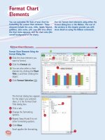
Margin Setting
Option
Pages
Lets you select the pages in the
worksheet you want to print.
Made Simple
Print Orientation Button
Lets you print pages in Portrait
(vertical) or Landscape
(horizontal) modes.
Print Button
Printer Button
Lets you select the
printer you want to use.
Collated Option
Lets you print pages
of multiple copies in
sequence or by page.
Scaling Option
Lets you resize the data as
a proportion of original.

Copies Box
Paper Size Option
Printer Properties
Lets you decide whether to print
in black and white and color,
among other options.
Office for Windows Made Simple
www.it-ebooks.info
For your convenience Apress has placed some of the front
matter material after the index. Please use the Bookmarks
and Contents at a Glance links to access them.
www.it-ebooks.info

iii

Contents at a Glance
Contents iv
About the Author x
About the Technical Reviewer xi
Acknowledgments xii
■Quick Start Guide 1
■Chapter 1: Introducing Excel 2010 27
■Chapter 2: Getting Around the Worksheet and Data Entry 31
■Chapter 3: Editing Data 63
■Chapter 4: Number Crunching 101: Functions, Formulas, and Ranges 73
■Chapter 5: For Appearance’s Sake: Formatting Your Data 103
■Chapter 6: Charting Your Data 155
■Chapter 7: Sorting and Filtering Your Data: Excel’s Database Features 195
■Chapter 8: PivotTables: Data Aggregation Without the Aggravation 219
■Chapter 9: Managing Your Workbook 261

■Chapter 10: Printing Your Worksheets: Hard Copies Made Easy 289
■Chapter 11: Automating Your Work with Macros 323
Index 339
www.it-ebooks.info




1
1

Quick Start Guide
Believe it or not, you’re looking at a book about one of the most widely owned—but
underused—programs on the planet: Microsoft Excel, the 2010 edition. Underused?
Yep, because even though millions of people around the globe apply Excel to a vast
range of daily tasks, most users still don’t appreciate the even wider range of things
Excel can do—once they nail down its basics and begin to glimpse the huge potential
that lurks behind all those cells and buttons.
What makes Excel is interesting, and even exciting, is that once you learn those basics
you can start to make things happen onscreen. It’s true—enter a number here, and
something happens over there; change the values contributing to a chart, and the chart
changes. Write some formulas, and you’ll suddenly see something there that wasn’t
there before—and that something can make your work easier and more productive.
Is it worth learning about? You bet; and this Quick Start Guide will introduce you to
Excel and point you to the places in this book where you can learn more about the
things you have to know in order to get the most you can out of the software. So let’s
get started.
The Excel Worksheet: What You’re Looking At
Click your way into Excel, and you’ll be brought face to face with a screen that looks like
Figure 1 (minus the descriptive captions, of course).

www.it-ebooks.info
QUICK START GUIDE
2

Figure 1. The Excel worksheet 
What you’re looking at is a large grid called a worksheet—and there’s a lot more of it
than you can see at one time. Don’t confuse the worksheet with the workbook, which is
the name for the whole Excel file; just as Word speaks of a document, Excel uses the
term workbook. Think of a worksheet, then, as a page in the larger workbook.
The worksheet is bordered by a collection of buttons, icons, and fields that may not
make all that much sense to you yet, so I’ll offer a few introductory words about them
and what’s behind them. And don’t worry, I’ll explain in more detail as we move on.
 Row headers: These are the row numbers lining the far left
of the grid. You need to know row numbers in order to
determine a cell’s address. A cell is the name given to all
those rectangles making up the grid; each cell has an
address, formed by the intersection of a row header and a
column header.
www.it-ebooks.info
QUICK START GUIDE
3


Column headers: These are the
letters bordering the top of the
grid. Cells have addresses such
as E34, A279, and the like (the letter always come first—e.g., there’s no cell
34E, which sounds like a seat on an airplane). It’s in those cells where you’ll be
entering your spreadsheet data.



Name box: Among other things, the
Name box records the current address
of the cell pointer, that thick rectangle
that highlights the cell to which you’ve traveled. In the accompanying
screenshot, the Name box lets us know we’re in cell B12.
 Formula bar: This white strip reveals the data you’ve entered in a cell (see
Figure 2). If you think you can already tell that simply by looking at the
actual cell, you’ll soon learn that that’s not always the case.

Figure 2. The formula bar
 Ribbon: This is a strip of buttons that, when clicked, carry out a wide
variety of actions on the spreadsheet (see Figure 3). For example, the
ribbon is responsible for formatting (i.e., changing the appearance of
numbers in cells to look like, say, $45.00 instead 45, or turning any cell
containing a number greater than 100 orange). Click any of the
headings above the ribbon—the command tabs—and the contents of
the ribbon changes, revealing a new set of buttons. Note that the
command tabs are subdivided into Home, Insert, Page Layout,
Formulas, Data, Review, View, and Add-Ins, as shown in Figure 3.

Figure 3. The ribbon
 Button groups: These are clusters of buttons that perform related
tasks. Figure 3 shows the contents of the Home tab, which contains the
button groups Clipboard, Font, Alignment, and so on. The arrows in the
figure point to the Alignment and Styles button groups.
www.it-ebooks.info
QUICK START GUIDE
4

 Quick Access toolbar: This is a
set of buttons—sort of a mini-
ribbon—that contains
important basic commands
you’re likely to use often. The advantage of the Quick
Access toolbar is that it remains onscreen even if the
contents of the ribbon beneath it change, and it can
be customized so that you can add buttons to
represent other commands you often use.
 Worksheet tabs: Back to the
worksheet concept, those
three inserts entitled Sheet1,
Sheet2, and Sheet3 tucked in
the lower left of the screen are worksheet tabs, representing the three
worksheets that make up an Excel workbook for starters. Clicking any
of these three will reveal another worksheet just like the others,
affording you another batch of all those cells. When you start Excel,
you’ll be brought to Sheet1 by default. You can add many more new
worksheets to the workbook if you need more space in which to store
still more information.
 Scroll buttons: These are four arrow-shaped buttons holding down the
lower right and far right of the worksheet screen (see Figure 4).
Clicking these moves the worksheet right/left and up/down on the
screen. Try them and you’ll see what they do.

Figure 4. Scroll buttons
www.it-ebooks.info
QUICK START GUIDE
5
 Select All button: Clicking that rectangle wedged

between the A and the 1 in the upper left of the screen
will select, or highlight, all the cells in your worksheet—
and why that might matter will be discussed soon.
 Status bar: This is the lower border of the worksheet, which contains
buttons enabling you to modify ways in which the worksheet can be
viewed, and which reports information about selected cells (see Figure
5). Note the mode indicator at the left of the status bar, a caption that
reports the activity you’re currently performing on the worksheet—
Enter (for data entry), Edit, Ready, and so forth. You’ll see what all that
means soon.

Figure 5. The status bar, at the bottom of the worksheet. The arrow points to the mode indicator
 Dialog box launchers: These are the small
arrows pinned to the lower-right corner of
some of the button groups. Clicking a
launcher opens a dialog box that offers
command options additional to the ones
shown in the group.


Cell pointer: This is the bold rectangle that indicates your
current position on the spreadsheet.


Key Tips: Accessing Buttons with the Keyboard
The standard way to access all those buttons filling Excel’s ribbon is simply to click your
mouse on the button you want.
NOTE: Unless otherwise stated, all mouse clicks utilize the left button.
But there’s a keyboard alternative to this technique, called key tips. If you press the Alt
key once, you’ll introduce a collection of initialed minibuttons—the key tips—to the

screen (see Figure 6).

Figure 6. Note the letters that now accompany each tab.
www.it-ebooks.info
QUICK START GUIDE
6
By typing any of the letters (or numbers, in some cases) shown, you’ll be brought to the
tab associated with that letter. Thus, if you press A, you’ll call up the Data tab, as shown
in Figure 7.

Figure 7. Take a letter: Accessing the Data tab with key tips
As shown, once you’ve accessed a tab, its button options can also be
accessed via the key tips, some of which require tapping two keys in
sequence. Thus, in Figure 7, pressing T will activate the Filter option
(something you’ll learn about in Chapter 7).
Moreover, if the button command you’ve selected fires up a drop-down
menu, those menu commands can likewise be accessed with key tips.
Thus, if you first tap H to access the Home tab and then press V to trigger
the Paste button, its drop-down menu options will also be accompanied
by key tips, as shown in the illustration.
NOTE: Clicking any button that features a small arrow will reveal a drop-down menu.
And each time you press the Esc key, you move back up one key tip level.
That means that in the preceding screenshot, pressing Esc will close the drop-
down menu and return you to all the Home tab key tips; pressing Esc again will
take you back to the original key tips pinned to each tab, and pressing Esc still
once more will turn off the key tips altogether.
Contextual Tabs
There’s another set of tabs that may suddenly materialize on the screen. Called
contextual tabs, these appear only when you’ve clicked certain objects, such as charts
(see Chapter 6) or PivotTables (Chapter 8), and bring along tabs containing buttons

specific to that object (see Figure 8).
www.it-ebooks.info
QUICK START GUIDE
7

Figure 8. The Chart Tools contextual tab (see the arrow at the top) and the Chart Tools tabs (see the lower arrow):
Design, Layout, and Format
The Chart Tools tab only appears when you click the chart. Click away from the
chart and the Chart Tools contextual tab disappears, to return only when you
click back on the chart. That’s what makes it contextual.
A Visit Backstage
Beginning with the 2010 release of Excel, a new green tab called File
has been added.
The File tab was introduced to replace the Office 2007 button, that
rather ambiguous circular object that was stationed at the upper left
of Excel’s screen.
Click the File tab and you’ll be brought to what’s called the Backstage—a large
behind-the-scenes area that houses commands that impact the workbook as a whole—
including printing (including a print preview), saving, and sending the workbook, as well
as sharing it with others (see Figure 9). It also offers numerous default settings that you
can change if you want (e.g., how many worksheets a new workbook will start with). The
www.it-ebooks.info
QUICK START GUIDE
8
Backstage also lists the workbooks you’ve recently accessed, so that you can click any
one on the list and open it again.

Figure 9. A print preview as displayed in the Backstage. Note the other Backstage options in the left columns.
TIP: To exit the Backstage and return to the worksheet, press the Esc key or just click any other
tab.

Customizing the Quick Access Toolbar
Now let’s get back to the Quick Access toolbar,
that downsized ribbon assigned to the upper left
of the worksheet screen.
To repeat, the Quick Access toolbar stores frequently used buttons—and again, what
makes the Quick Access toolbar so handy is that, unlike the larger tabs sitting beneath
it, it’s always there, along with its buttons, of course.
What makes the Quick Access toolbar even handier is that you can post additional
buttons there, so they too will always remain in view and available.
There are several ways in which you can customize the Quick Access toolbar with
additional buttons.
www.it-ebooks.info
QUICK START GUIDE
9
For one, you can click the small arrow at the far right of the
Quick Access toolbar, revealing the menu shown in the
accompanying screenshot.
The menu offers just a small sample of all of Excel’s
commands, but these are among the more popular ones. Just
click the commands you want to install, and buttons
representing your selections will appear on the Quick Access
toolbar.
You can right-click virtually any button on any Excel tab,
calling up the menu shown here.
In this case the currency format button has been
clicked, which gives numbers a currency-like
appearance (e.g., 45.23 might be changed into
$45.23).
Now that button will also show up in the Quick Access
toolbar.

If you click the File tab to enter the Backstage, and then click Options  Quick Access
Toolbar, you’ll see the dialog shown in Figure 10.
www.it-ebooks.info
QUICK START GUIDE
10

Figure 10. Another route to adding buttons to the Quick Access toolbar—via the Backstage
Figure 10 shows a very long list of Excel commands, any of which you can select with
your mouse and then click Add in order to install it onto the Quick Access toolbar.
Figure 11 shows the Spelling command being selected and added it to the Quick
Access toolbar, which is done by clicking the Add button.

Figure 11. Adding the Spelling button to the Quick Access toolbar
www.it-ebooks.info
QUICK START GUIDE
11
Try it yourself. Select Spelling and click Add, and the Spelling button will be added to
the right-hand Customize Quick Access Toolbar column, as shown in Figure 12.

Figure 12. There it is!
Click OK, and the button will take its place in the Quick
Access toolbar , as shown in the accompanying
illustration.
To remove a button from the Quick Access toolbar ,
just right-click the button and select the first option
on the resulting menu, as shown in the illustration to
the right.

NOTE: By default, adding a button to the Quick Access toolbar makes that button available on the
Quick Access toolbar in all your workbooks. If you want to restrict the button’s appearance to the

Quick Access toolbar of the current workbook only, you need to click the drop-down arrow by the
Customize Quick Access field and click the name of the particular workbook (see Figure 13).
www.it-ebooks.info
QUICK START GUIDE
12

Figure 13. Adding a button to the Quick Access toolbar for a particular workbook only
Where to Learn More
Table1 lists the major Excel topics you’ll find discussed in this book, and where to find
them.
Table 1. Major Excel Topics
Topic Illustration Where to Learn More (Chapter and Section)
Navigating the
worksheet

Chapter 2, “Getting Around a Worksheet”
Entering text data
in cells

Chapter 2, “Entering Text and Data”
Selecting (or
highlighting) cells

Chapter 2, “Selecting Multiple Cells”
Getting text to fit in
columns

Chapter 2, “Widening and Narrowing
Columns”
Entering numerical

data

Chapter 2, “Entering Numerical Data: How
It’s Different”
Validating data

Chapter 2, “Data Validation: Bringing
Quality Control to the Worksheet”

Constructing a
drop-down menu

Chapter 2, “Making a List: Personalizing a
Drop-Down Menu”
Making changes to
data in cells

Chapter 3, “Changing Your Data”
www.it-ebooks.info
QUICK START GUIDE
13
Topic Illustration Where to Learn More (Chapter and Section)
Copying and
moving data

Chapter 3, “Copying and Moving:
Duplicating and Relocating Your Data”
Writing formulas

Chapter 4, “Customizing the Worksheet

with Formulas”
Using functions

Chapter 4, “Automatic Calculations with
Functions”
Copying and
moving formulas

Chapter 4, “Copying Formulas: More Than
Just Duplication”
Working with
relative and
absolute cell
references
$N6*A2

Chapter 4, “Keeping a Cell Reference
Constant with Absolute Addressing”
Pasting values

Chapter 4, “Copying a Formula’s Result
Only”
Changing font
appearances

Chapter 5, “Basic Formatting”
Changing cell
alignment

Chapter 5, “Aligning (and Realigning) Your

Data”
Wrapping text in
its cell

Chapter 5, “Wrapping Text”
www.it-ebooks.info
QUICK START GUIDE
14
Topic Illustration Where to Learn More (Chapter and Section)
Merging and
centering cells

Chapter 5, “Adding a Title with Merge and
Center”
Inserting columns
and rows

Chapter 5, “Inserting, Deleting, and Hiding
Columns and Rows”
Formatting
numeric data

Chapter 5, “Formatting Values: Making the
Numbers Look Good”
Working with dates

Chapter 5, “Working with Dates: Dates Are
Numbers Too”
Using the format
painter

Chapter 5, “Copying Formats (Not Data)
with the Format Painter”

Using cell styles

Chapter 5, “Applying Ready-Made Formats
with Styles”

Working with
conditional
formatting


Chapter 5, “Conditional Formatting”

Understanding
chart types

Chapter 6, “Choosing a Chart Type”
www.it-ebooks.info
QUICK START GUIDE
15
Topic Illustration Where to Learn More (Chapter and Section)
Constructing a
chart

Chapter 6, “Creating a Column Chart”
Changing a chart

Chapter 6, “Changing a Chart”
Changing the
default chart

Chapter 6, “Changing the Default Chart”
Changing chart
formatting

Chapter 6, “Formatting Charts”
Adding a chart title

Chapter 6, “Adding Extra Chart Elements
with the Layout Tab”
Working with
sparklines

Chapter 6, “Introducing Sparklines: Mini-
Charts Placed in Cells”

Sorting data

Chapter 7, “Sorting Data: Instilling Order in
Your Data”
Filtering data

Chapter 7, “Finding What You Want with
Filters”

Using tables

Chapter 7, “Tables: Adding User-
Friendliness to Your Database”

www.it-ebooks.info
QUICK START GUIDE
16
Topic Illustration Where to Learn More (Chapter and Section)
Formatting and
styling tables

Chapter 7, “Tables: Adding User-
Friendliness to Your Database”

Removing
duplicate records
in a table

Chapter 7, “Finding Duplicate Records in
the Table (and Removing Them)”
Learning what
PivotTables can do

Chapter 8, “Looking at Some PivotTables”

Constructing a
PivotTable

Chapter 8, “Creating a PivotTable”

Grouping

PivotTable data

Chapter 8, “Grouping PivotTable Data:
Organizing Your Time(s)”

Adding new
records to the
PivotTable

Chapter 8, “Refreshing the PivotTable:
Changing the Data”

Learning how to
use the Slicer

Chapter 8, “Viewing which Records Are
Filtered: Using the Slicer”

Formatting a
PivotTable

Chapter 8, “Formatting the PivotTable”

www.it-ebooks.info
QUICK START GUIDE
17
Topic Illustration Where to Learn More (Chapter and Section)
Devising a
PivotChart

Chapter 8, “Creating Charts from
PivotTables Using PivotCharts”

Adding and
moving new
worksheets

Chapter 9, “Adding and Moving New
Worksheets”

Hiding and
unhiding
worksheets

Chapter 9, “Hiding Sheets”
Grouping sheets

Chapter 9, “Grouping Sheets: Changing
Multiple Sheets at the Same Time”

Writing formulas
with cells in
different
worksheets

Chapter 9, “Referring to Cells in Other
Worksheets: Using Them in Formulas”
Displaying or
hiding gridlines,
headings, and

formulas

Chapter 9, “Using the View Context Tab to
Show and Hide Basic Screen Elements”

Freezing screen
panes

Chapter 9, “Keeping Important Data in
View with the Freeze Panes Option”

Protecting
worksheets and
workbooks

Chapter 9, “Protecting the Worksheet and
the Workbook”

Printing the entire
worksheet

Chapter 10, “Printing the Entire
Worksheet”
Printing a selected
range of the
worksheet

Chapter 10, “Printing a Selection”
www.it-ebooks.info
QUICK START GUIDE

18
Topic Illustration Where to Learn More (Chapter and Section)
Working with the
Print Backstage

Chapter 10, “Surveying Printing Options:
The Print Backstage”
Setting the print
area

Chapter 10, “Setting the Print Area”
Imposing a page
break

Chapter 10, “Working with Page Breaks”
Working with page
break previews

Chapter 10, “Previewing the Page Break:
Getting a Bird’s-Eye View of the Printout”

Working with
headers and
footers

Chapter 10, “Adding Headers and Footers”
Recording and
editing basic
macros

Chapter 11
Excel Keyboard Equivalents
Because there are so many things you can do with Excel, it naturally needs to offer its
users a long list of commands—and along with them, a long list of keyboard equivalents.
Needless to say, you may never have to use some of these, but they’re available, and as
your knowledge of Excel expands you may want to explore more of them. Table 2 lists a
lengthy assortment of keyboard equivalents that employ the Ctrl key. While you may not
www.it-ebooks.info
QUICK START GUIDE
19
yet understand what some of them do, by the time your reach the end of this book they
should make a lot more sense.
Table 2. Ctrl Key Shortcuts
Ctrl Key Combination What It Does
Ctrl+Shift+) Unhides any hidden columns within the selection.
Ctrl+Shift+( Unhides any hidden rows within the selection.
Ctrl+Shift+~ Applies the General number format.
Ctrl+Shift+$ Applies the Currency format with two decimal places (negative numbers in
parentheses).
Ctrl+Shift+% Applies the Percentage format with no decimal places.
Ctrl+Shift+! Applies the Number format with two decimal places, a thousands
separator, and a minus sign (–) for negative values.
Ctrl+Shift+: Enters the current time; that is, the actual time as data, not a formula result.
Ctrl+Shift+" Copies the value from the cell above the active cell into the cell or the
formula bar. That is, if you click in a blank cell, this shortcut will copy any
value in the cell immediately above it. If that value is the result of a formula,
this shortcut will paste only that value, not the formula.
Ctrl+; Enters the current date as data, not a formula result.
Ctrl+` Alternates between displaying cell values and displaying formulas in the
worksheet. That is, this shortcut will display a cell formula on the screen

instead of its value. Tap the shortcut a second time and the value will
return. This option is available for the workbook via File  Advanced  Show
formulas in cells instead of their calculated results.
Ctrl+' Copies the formula from the cell above the active cell into selected cells or
the formula bar. The copied formula cell references change as per relative
cell references. You need to select the source cell along with the
destination cells at the same time.
Ctrl+1 Displays the Format Cells dialog box.
Ctrl+5 Applies or removes a strikethrough effect through characters populating
cells.
Ctrl+9 Hides the selected rows.
Ctrl+0 Hides the selected columns.
www.it-ebooks.info
QUICK START GUIDE
20
Ctrl Key Combination What It Does
Ctrl+A

Selects the entire worksheet. If the worksheet contains data, Ctrl+A selects
the current region—that is, an area of cells populated by data (e.g., a
table)—if you click in that region. Pressing Ctrl+A a second time selects the
entire worksheet. If you click in a blank area of the worksheet, Ctrl+A will
initially select the entire worksheet.
Ctrl+B

Applies or removes bold formatting with alternating taps.
Ctrl+C

Copies the selected cells.
Ctrl+D

Uses the Fill Down command to copy the contents and format of the
topmost cell of a selected range into the cells immediately below.
Ctrl+F

Displays the Find and Replace dialog box, with the Find tab selected. This
works similarly to the Find and Replace option in Word. This dialog is also
available via the Find & Select option in the Editing button group on the Home
tab.
Ctrl+Shift+F

Opens the Format Cells dialog box with the Font tab selected.
Ctrl+G

Displays the Go To dialog box (as does F5).
Ctrl+H

Displays the Find and Replace dialog box, with the Replace tab selected.
Ctrl+I

Applies or removes italic formatting with alternating taps.
Ctrl+L

Displays the Create Table dialog box (equivalent to Ctrl+T).
Ctrl+N

Creates a new, blank workbook.
Ctrl+O

Displays the Open dialog box to open or find a file.

Ctrl+P

Displays the Print tab in Microsoft Office Backstage view.
Ctrl+R

Uses the Fill Right command to copy the contents and format of the
leftmost cell of a selected range into the cells to the right.
Ctrl+S

Saves the active file with its current file name, location, and file format.
Ctrl+T

Displays the Create Table dialog box.
Ctrl+U

Applies or removes underlining with alternating taps.
Ctrl+V

Performs the classic Paste command. Pressing Ctrl+V inserts the contents
of the Clipboard at the insertion point and replaces any selection. This
option is available only after you have cut or copied text, cell contents, or
an object.
www.it-ebooks.info
QUICK START GUIDE
21
Ctrl Key Combination What It Does
Ctrl+Alt+V

Displays the Paste Special dialog box, enabling you to paste only the results
of a copied formula, by clicking the Values option in the dialog box. If, for

example, a formula in cell A17 states =SUM(A2:A13) and yields 3224, Paste
Special will return only the value 3224 in the destination cell. It will not copy
the formula. This option is also available via the Paste button on the Home
tab and on the Paste shortcut menu.
Ctrl+W

Closes the selected workbook window.
Ctrl+X

Cuts the selected cells
Ctrl+Y

Performs a redo; that is, it undoes the last command you’ve undone via
Undo. But it also repeats any last command or action, if possible.
CTR+Z Uses the Undo command to reverse the last action or delete the last entry
you typed. Successive presses of Ctrl+Z continue to undo the immediately
previous command.
The shortcuts shown in Table 3 work with the function keys (the “F” keys stationed in
the upper row of your keyboard).
Table 3. Function Key Shortcuts
Function Key What It Does
F1

Displays the Excel Help task pane.
Ctrl+F1 displays or hides the ribbon.
Alt+F1 creates a chart of the data in a current range in which you’ve clicked, on
the worksheet containing the data.
Alt+Shift+F1 inserts a new worksheet.
F2

Edits the active cell and positions the insertion point at the end of the cell
contents. It also moves the insertion point into the formula bar when the
capability to edit in a cell is turned off. This keystroke draws a temporary border
around the cells that contribute to any formula in the cell you’re editing. Thus,
tapping F2 while in a cell containing =AVERAGE(A6:A10) will trace a border
around cells A6:A10. It provides an easy way to identity cell relationships.
Shift+F2 adds or edits a cell comment.
Ctrl+F2 displays the print preview area on the Print tab in the Backstage view (as
does Ctrl+P).
F3

Displays the Paste Name dialog box. This option is only available if there are
range names in the workbook.
Shift+F3 displays the Insert Function dialog box.
www.it-ebooks.info
QUICK START GUIDE
22
Function Key What It Does
F4

Repeats the last command or action, if possible.
Ctrl+F4 closes the selected workbook window, as does Ctrl+W.
Alt+F4 closes Excel. As usual, you’ll will be prompted to save your changes
should you not have already done so.
F5

Displays the Go To dialog box.
Ctrl+F5 restores the window size of the selected workbook window.
F6

Switches between the worksheet, ribbon, task pane, and zoom controls. In a
worksheet that has been split, F6 includes the split panes when switching
between panes and the ribbon area. (You can split a worksheet via View 
Manage This Window  Freeze Panes  Split Window.)
Shift+F6 switches between the worksheet, zoom controls, task pane, and ribbon.
Ctrl+F6 switches to the next workbook window when more than one workbook
window is open.
F7

Displays the Spelling dialog box to check spelling in the active worksheet or
selected range.
F8

Turns Extend mode on or off. In Extend mode, “Extended Selection” appears in
the status line, and the arrow keys extend the selection. Extend mode allows
you to select consecutive cells with the keyboard arrow keys without requiring
you to hold down the Shift key. Tapping F8 a second time toggles this
command off.
Shift+F8 enables you to add a nonadjacent cell or range to a selection of cells
by using the arrow keys. That is, after having selected one range, tapping this
shortcut lets you click elsewhere and drag or key-select another range, even as
the original range remains selected.
Alt+F8 displays the Macro dialog box, for creating, running, editing, or deleting a
macro.
F9

Calculates all worksheets in all open workbooks. You’ll rarely use this one
nowadays. You might, however, if your workbook features thousands of
formulas. When you enter new data, Excel recalculates every formula whose
result has changed since the last calculation. On a slow computer, that process

can be rather time-consuming. If this is the case, you can click Formulas 
Calculation  Calculation Options  Manual, which prevents Excel from recalculating
formulas when you enter new data. F9 will then calculate the worksheet when
pressed. The Calculate Now button in the Calculation button group calculates the
workbook in which you’ve clicked.
Shift+F9 calculates the active worksheet.
Ctrl+Alt+F9 calculates all worksheets in all open workbooks, regardless of
whether they have changed since the last calculation.
Ctrl+F9 minimizes a workbook window to an icon.
www.it-ebooks.info