Sheldon axler, paul bourdon, wade ramey harmonic function theory (2001) 978 1 4757 8137 3
Bạn đang xem bản rút gọn của tài liệu. Xem và tải ngay bản đầy đủ của tài liệu tại đây (21.94 MB, 266 trang )
Graduate Texts in Mathematics
S. Axler
Editorial Board
F.W. Gehring K.A. Ribet
Springer Science+Business Media, LLC
www.pdfgrip.com
137
Graduate Texts in Mathematics
2
3
4
5
6
7
8
9
10
II
12
13
14
15
16
17
18
19
20
21
22
23
24
25
26
27
28
29
30
31
32
33
34
TAKEUTUZARING. Introduction to
Axiomatic Set Theory. 2nd ed.
OXTOBY. Measure and Category. 2nd ed.
SCHAEFER. Topological Vector Spaces.
2nd ed.
HILTON/STAMMBACH. A Course in
Homological Algebra. 2nd ed.
MAc LANE. Categories for the Working
Mathematician. 2nd ed.
HUGHESIPIPER. Projective Planes.
SERRE. A Course in Arithmetic.
TAKEUTUZARING. Axiomatic Set Theory.
HUMPHREYS. Introduction to Lie Algebras
and Representation Theory.
COHEN. A Course in Simple Homotopy
Theory.
CONWAY. Functions of One Complex
Variable I. 2nd ed.
BEALS. Advanced Mathematical Analysis.
ANDERSONIFULLER. Rings and Categories
of Modules. 2nd ed.
GOLUBITSKy/GUlLLEMIN. Stable Mappings
and Their Singularities.
BERBERIAN. Lectures in Functional
Analysis and Operator Theory.
WINTER. The Structure of Fields.
ROSENBLATT. Random Processes. 2nd ed.
HALMOS. Measure Theory.
HALMOS. A Hilbert Space Problem Book.
2nd ed.
HUSEMOLLER. Fibre Bundles. 3rd ed.
HUMPHREYS. Linear Algebraic Groups.
BARNES/MACK. An Algebraic Introduction
to Mathematical Logic.
GREUB. Linear Algebra. 4th ed.
HOLMES. Geometric Functional Analysis
and Its Applications.
HEWITT/STROMBERG. Real and Abstract
Analysis.
MANES. Algebraic Theories.
KELLEY. General Topology.
ZARISKIISAMUEL. Commutative Algebra.
Vol.I.
ZARISKIISAMUEL. Commutative Algebra.
VoU!.
JACOBSON. Lectures in Abstract Algebra I.
Basic Concepts.
JACOBSON. Lectures in Abstract Algebra II.
Linear Algebra.
JACOBSON. Lectures in Abstract Algebra
Ill. Theory of Fields and Galois Theory.
HIRSCH. Differential Topology.
SPITZER. Principles of Random Walk.
2nd ed.
35 ALEXANDERiWERMER. Several Complex
Variables and Banach Algebras. 3rd ed.
36 KELLEy/NAMIOKA et al. Linear
Topological Spaces.
37 MONIC Mathematical Logic.
38 GRAUERTIFRITZSCHE. Several Complex
Variables.
39 ARVESON. An Invitation to C·-Algebras.
40 KEMENy/SNELLIKNAPP. Denumerable
Markov Chains. 2nd ed.
41 ApOSTOL. Modular Functions and Dirichlet
Series in Number Theory.
2nded.
42 SERRE. Linear Representations of Finite
Groups.
43 GILLMAN/JERISON. Rings of Continuous
Functions.
44 KENDIG. Elementary Algebraic Geometry.
45 LoEvE. Probability Theory I. 4th ed.
46 LoEvE. Probability Theory II. 4th ed.
47 MOISE. Geometric Topology in
Dimensions 2 and 3.
48 SAOISlWu. General Relativity for
Mathematicians.
49 GRUENBERGIWEIR. Linear Geometry.
2nd ed.
50 EDWARDS. Fermat's Last Theorem.
51 KLINGENBERG. A Course in Differential
Geometry.
52 HARTSHORNE. Algebraic Geometry.
53 MANlN. A Course in Mathematical Logic.
54 GRAVERiW ATKINS. Combinatorics with
Emphasis on the Theory of Graphs.
55 BROWNIPEARCY. Introduction to Operator
Theory I: Elements of Functional
Analysis.
56 MASSEY. Algebraic Topology: An
Introduction.
57 CROWELLIFox. Introduction to Knot
Theory.
58 KOBLITZ. p-adic Numbers, p-adic Analysis,
and Zeta-Functions. 2nd ed.
59 LANG. Cyclotomic Fields.
60 ARNOLD. Mathematical Methods in
Classical Mechanics. 2nd ed.
61 WHITEHEAD. Elements of Homotopy
Theory.
62 KARGAPOLOvIMERLZJAKOV. Fundamentals
of the Theory of Groups.
63 BOLLOBAS. Graph Theory.
64 EDWARDS. Fourier Series. Vol. I. 2nd ed.
65 WELLS. Differential Analysis on Complex
Manifolds. 2nd ed.
www.pdfgrip.com
(continued ajier index)
Sheldon Axler
Paul Bourdon
Wade Ramey
Harmonic Function
Theory
Second Edition
With 21 Illustrations
t
Springer
www.pdfgrip.com
Sheldon Axler
Mathematics Department
San Francisco State University
San Francisco, CA 94132
USA
Paul Bourdon
Mathematics Department
Washington and Lee University
Lexington, VA 24450
USA
Wade Ramey
8 Bret Harte Way
Berkeley, CA 94708
USA
Editorial Board
S. Axler
Mathematics Department
San Francisco State
University
San Francisco, CA 94132
USA
F.W. Gehring
Mathematics Department
East Hall
University of Michigan
Ann Arbor, MI 48109
USA
K.A. Ribet
Mathematics Department
University of California
at Berkeley
Berkeley, CA 94720-3840
USA
Mathematics Subject Classification (2000): 31-01, 31B05, 31C05
Library of Congress Cataloging-in-Publication Data
Axler, Sheldon Jay.
Harmonic function theory/Sheldon Axler, Paul Bourdon, Wade Ramey.-2nd ed.
p. cm. - (Graduate texts in mathematics; 137)
Includes bibliographical references and indexes.
ISBN 978-1-4419-2911-2
ISBN 978-1-4757-8137-3 (eBook)
DOI 10.1007/978-1-4757-8137-3
1. Harmonic functions. I. Bourdon, Paul. II. Ramey, Wade.
QA405 .A95 2001
515'.53-dc21
© 200 I, 1992 Springer Science+Business Media New York
Originally published by Springer-Verlag New York, Inc. in 2001
Softcover reprint of the hardcover 2nd edition 200 I
III. Title.
IV. Series.
00-053771
All rights reserved. This work may not be translated or copied in whole or in part without the
written permission of the publisher Springer Science+Business Media, LLC,
except for brief. excerpts in connection with reviews or scholarly analysis. Use
in connection with any form of information storage and retrieval, electronic adaptation, computer
software, or by similar or dissimilar methodology now known or hereafter developed is forbidden.
The use of general descriptive names, trade names, trademarks, etc., in this publication, even if the
former are not especially identified, is not to be taken as a sign that such names, as understood by
the Trade Marks and Merchandise Marks Act, may accordingly be used freely by llQyone.
This reprint has been authorized by Springer-Verlag (BerlinlHeidelberg/New York) for sale in
the People's Republic of China only and not for export therefrom.
Reprinted in China by Beijing World Publishing Corporation, 2004
98765 432 I
ISBN 978-1-4419-2911-2
SPIN 10791946
www.pdfgrip.com
Cantents
Preface
ix
Acknowledgments
xi
CHAPTER 1
Basic Properties of Harmonic Functions
Definitions and Examples . . . . . . . . . . . . . . . . . . . . . . .
lnvariance Properties . . . . . . . . . . . . . . . . . . . . . . . . ..
The Mean-Value Property. . . . . . . . . . . . . . . . . . . . . . ..
The Maximum Principle. . . . . . . . . . . . . . . . . . . . . . . ..
The Poisson Kernelfor the Ball . . . . . . . . . . . . . . . . . . ..
The Dirichlet Problem for the Ball . . . . . . . . . . . . . . . . ..
Converse of the Mean-Value Property . . . . . . . . . . . . . . ..
Real Analyticity and Homogeneous Expansions . . . . . . . . ..
Origin of the Term "Harmonic" . . . . . . . . . . . . . . . . . . ..
Exercises. . . . . . . . . . . . . . . . . . . . . . . . . . . . . . . . ..
1
1
2
4
7
9
12
17
19
25
26
CHAPTER 2
Bounded Harmonic Functions
liouville's Theorem. . . . . . . . . . . . . . . . . . . . . . . . . ..
Isolated Singularities .. . . . . . . . . . . . . . . . . . . . . . . ..
Cauchy's Estimates . . . . . . . . . . . . . . . . . . . . . . . . . . .
Normal Families . . . . . . . . . . . . . . . . . . . . . . . . . . . ..
Maximum Principles. . . . . . . . . . . . . . . . . . . . . . . . . ..
Limits Along Rays . . . . . . . . . . . . . . . . . . . . . . . . . . ..
Bounded Harmonic Functions on the Ball. . . . . . . . . . . . ..
Exercises . . . . . . . . . . . . . . . . . . . . . . . . . . . . . . . . ..
v
www.pdfgrip.com
31
31
32
33
35
36
38
40
42
Contents
vi
CHAPTER
3
Positive Harmonic Functions
Liouville's Theorem . . . . . . . . . . . . . . . .
Harnack's Inequality and Harnack's Principle
Isolated Singularities . . . . . . . . . . . . . . .
Positive Harmonic Functions on the Ball . . .
Exercises. . . . . . . . . . . . . . . . . . . . . . .
..
..
..
..
..
45
45
47
50
55
56
..
..
..
..
..
..
..
59
59
61
62
63
66
67
71
Harmonic Polynomials
Polynomial Decompositions . . . . . . . . . . . . . . . . . . . . ..
Spherical Harmonic Decomposition of L 2 (5) . . . . . . . . . . .
Inner Product of Spherical Harmonics. . . . . . . . . . . . . . ..
Spherical Harmonics Via Differentiation . . . . . . . . . . . . ..
Explicit Bases of .1fm (R n ) and .1fm (5) . . . . . . . . . . . . . . .
Zonal Harmonics . . . . . ". . . . . . . . . . . . . . . . . . . . . . ..
The Poisson Kernel Revisited . . . . . . . . . . . . . . . . . . . ..
A Geometric Characterization of Zonal Harmonics . . . . . . . .
An Explicit Formula for Zonal Harmonics . . . . . . . . . . . . .
Exercises . . . . . . . . . . . . . . . . . . . . . . . . . . . . . . . . . .
73
74
78
82
85
92
94
97
100
104
106
.
.
.
.
.
.
.
.
.
.
.
.
.
.
.
.
.
.
.
.
.
.
.
.
.
.
.
.
.
.
.
.
.
.
.
.
.
.
.
.
.
.
.
.
.
CHAPTER 4
The Kelvin Transform
Inversion in the Unit Sphere. . . . . . . . . . . . . . . .
Motivation and Definition . . . . . . . . . . . . . . . . .
The Kelvin Transform Preserves Harmonic Functions
Harmonicity at Infinity . . . . . . . . . . . . . . . . . . .
The Exterior Dirichlet Problem . . . . . . . . . . . . . .
Symmetry and the Schwarz Reflection Principle. . . .
Exercises. . . . . . . . . . . . . . . . . . . . . . . . . . . .
.
.
.
.
.
.
.
.
.
.
.
.
.
.
.
.
.
.
.
.
.
.
.
.
.
.
.
.
CHAPTER 5
CHAPTER
6
Harmonic Hardy Spaces
Poisson Integrals of Measures . . . . . . . . . . . . . . . . . . . . .
Weak* Convergence . . . . . . . . . . . . . . . . . . . . . . . . . . .
The Spaces h P (B) . . . . . . . . . . . . . . . . . . . . . . . . . . . .
The Hilbert Space h 2 (B) . . . . . . . . . . . . . . . . . . . . . . . .
The Schwarz Lemma . . . . . . . . . . . . . . . . . . . . . . . . . .
The Fatou Theorem . . . . . . . . . . . . . . . . . . . . . . . . . . .
Exercises . . . . . . . . . . . . . . . . . . . . . . . . . . . . . . . . . .
www.pdfgrip.com
111
III
115
117
121
123
128
138
Contents
CHAPTER
vii
7
Harmonic Functions on Half-Spaces
The Poisson Kernel for the Upper Half-Space . . . . . . . . . . .
The Dirichlet Problem for the Upper Half-Space . . . . . . . . . .
The Harmonic Hardy Spaces h P (H) . . . . . . . . . . . . . . ...
From the Ball to the Upper Half-Space, and Back . . . . . . . . .
Positive Harmonic Functions on the Upper Half-Space ......
Nontangential limits . . . . . . . . . . . . . . . . . . . . . . . . . .
The Local Fatou Theorem . . . . . . . . . . . . . . . . . . . . . . .
Exercises . . . . . . . . . . . . . . . . . . . . . . . . . . . . . . . . . .
CHAPTER
143
144
146
151
153
156
160
161
167
8
Harmonic Bergman Spaces
171
Reproducing Kernels . . . . . . . . . . . . . . . . . . . . . . . . . . 172
The Reproducing Kernel of the Ball . . . . . . . . . . . . . . . . . 176
Examples in bP(B) . . . . . . . . . . . . . . . . . . . . . . . . . . . . 181
The Reproducing Kernel of the Upper Half-Space . . . . . . . . . 185
Exercises . . . . . . . . . . . . . . . . . . . . . . . . . . . . . . . . . . 188
CHAPTER
9
The Decomposition Theorem
191
The Fundamental Solution of the Laplacian . . . . . . . . . . . . 191
Decomposition of Harmonic Functions . . . . . . . . . . . . . . . 193
Bacher's Theorem Revisited . . . . . . . . . . . . . . . . . . . . . . 197
Removable Sets for Bounded Harmonic Functions .'. . . . . . . 200
The Logarithmic Conjugation Theorem . ; . . . . . . . . . . . . . 203
Exercises . . . . . . . . . . . . . . . . . . . . ..... ' . . . . . . . . . 206
CHAPTER
10
Annular Regions
209
Laurent Series . . . . . . . . . . . . . . . . . . . . . . . . . . . . . . . 209
Isolated Singularities . . . . . . . . . . . . . . . . . . . . . . . . . . 210
The Residue Theorem. . . . . . . . . . . . . . . . . . . . . . . . . . 213
The Poisson Kernel for Annular Regions . . . . . . . . . . . . . . 215
Exercises . . . . . . . . . . . . . . . . . . . . . . . . . . . . . . . . . . 219
CHAPTER 11
The Dirichlet Problem and Boundary Behavior
223
The Dirichlet Problem . . . . . . . . . . . . . . . . . . . . . . . . . . 223
Subharmonic Functions . . . . . . . . . . . . . . . . . . . . . . . . . 224
www.pdfgrip.com
Contents
viii
The Perron Construction . . . . . . . . . . . . . . . . . . . . . . . .
Barrier Functions and Geometric Criteria for Solvability ....
Nonextendability Results . . . . . . . . . . . . . . . . . . . . . . . .
Exercises . . . . . . . . . . . . . . . . . . . . . . . . . . . . . . . . . .
226
227
233
236
APPENDIX A
Volume, Surface Area, and Integration on Spheres
Volume of the Ball and Surface Area of the Sphere . . . . . . . .
Slice Integration on Spheres . . . . . . . . . . . . . . . . . . . . . .
Exercises . . . . . . . . . . . . . . . . . . . . . . . . . . . . . . . . . .
239
239
241
244
APPENDIX B
Harmonic Function Theory and Mathematica
247
References
249
Symbol Index
251
Index
255
www.pdfgrip.com
Preface
Harmonic functions-the solutions of Laplace's equation-playa
crucial role in many areas of mathematics, physics, and engineering.
But learning about them is not always easy. At times the authors have
agreed with Lord Kelvin and Peter Tait, who wrote ([18], Preface)
There can be but one opinion as to the beauty and utility of this
analysis of Laplace; but the manner in which it has been hitherto
presented has seemed repulsive to the ablest mathematicians, and
difficult to ordinary mathematical students.
The quotation has been included mostly for the sake of amusement,
but it does convey a sense of the difficulties the uninitiated sometimes
encounter.
The main purpose of our text, then, is to make learning about harmonic functions easier. We start at the beginning of the subject, assuming only that our readers have a good foundation in real and complex
analysis along with a knowledge of some basic results from functional
analysis. The first fifteen chapters of [15], for example, provide sufficient preparation.
In several cases we simplify standard proofs. For example, we replace the usual tedious calculations showing that the Kelvin transform
of a harmonic function is harmonic with some straightforward observations that we believe are more revealing. Another example is our
proof of Bacher's Theorem, which is more elementary than the classical proofs.
We also present material not usually covered in standard treatments
of harmonic functions (such as [9], [11], and [19]). The section on the
Schwarz Lemma and the chapter on Bergman spaces are examples. For
ix
www.pdfgrip.com
x
Preface
completeness, we include some topics in analysis that frequently slip
through the cracks in a beginning graduate student's curriculum, such
as real-analytic functions.
We rarely attempt to trace the history of the ideas presented in this
book. Thus the absence of a reference does not imply originality on
our part.
For this second edition we have made several major changes. The
key improvement is a new and considerably simplified treatment of
spherical harmonics (Chapter 5). The book now includes a formula for
the Laplacian of the Kelvin transform (Proposition 4.6). Another addition is the proof that the Dirichlet problem for the half-space with
continuous boundary data is solvable (Theorem 7.11), with no growth
conditions required for the boundary function. Yet another significant change is the inclusion of generalized versions of Liouville's and
Bacher's Theorems (Theorems 9.10 and 9.11), which are shown to be
equivalent. We have also added many exercises and made numerous
small improvements.
In addition to writing the text, the authors have developed a software package to manipulate many of the expressions that arise in harmonic function theory. Our software package, which uses many results
from this book, can perform symbolic calculations that would take a
prohibitive amount of time ifdone without a computer. For example,
the Poisson integral of any polynOmial can be computed exactly. Appendix B explains how readers can obtain our software package free of
charge.
The roots of this book lie in a graduate course 'at Michigan State
University taught by one of the authors and attended by the other authors along with a number of graduate students. The topic of harmonic
functions was presented with the intention of moving on to different
material after introducing the basic concepts. We did not move on to
different material. Instead, we began to ask natural questions about
harmonic functions. Lively and illuminating discussions ensued. A
freewheeling approach to the course developed; answers to questions
someone had raised in class or in the hallway were worked out and then
presented in class (or in the hallway). Discovering mathematics in this
way was a thoroughly enjoyable experience. We will consider this book
a success if some of that enjoyment shines through in these pages.
www.pdfgrip.com
Our book has been improved by our students and by readers of the
first edition. We take this opportunity to thank them for catching errors
and making useful suggestions.
Among the many mathematicians who have influenced our outlook
on harmonic function theory, we give special thanks to Dan Luecking
for helping us to better understand Bergman spaces, to Patrick Ahern
who suggested the idea for the proof of Theorem 7.11, and to Elias
Stein and Guido Weiss for their book [16], which contributed greatly to
our knowledge of spherical harmonics.
We are grateful to Carrie Heeter for using her expertise to make old
photographs look good.
At our publisher Springe~ we thank the mathematics editors Thomas
von Foerster (first edition) and Ina Lindemann (second edition) for their
support and encouragement, as well as Fred Bartlett for his valuable
assistance with electronic production.
xi
www.pdfgrip.com
CHAPTER 1
13asic 'Proyerties of
J-{armonic Junctions
'Definitions ana 'ExanyJ{es
Harmonic functions, for us, live on open subsets of real Euclidean
spaces. Throughout this book, n will denote a fixed positive integer
greater than 1 and 0 will denote an open, nonempty subset of Rn. A
twice continuously differentiable, complex-valued function u defined
on 0 is harmonic on 0 if
~u=O,
where ~ = Dl2 + ... + Dn 2 and D / denotes the second partial derivative
with respect to the ph coordinate variable. The operator ~ is called the
Laplacian, and the equation ~u = 0 is called Laplace's equation. We
say that a function u defined on a (not necessarily open) set E c Rn is
harmonic on E if u can be extended to a function harmonic on an open
set containing E.
We let x = (Xl, ... ,xn ) denote a typical point in R n and let Ixi =
(Xl 2 + ... + Xn 2 )l/2 denote the Euclidean norm of x.
The simplest nonconstant harmonic functions are the coordinate
functions; for example, u(x) = Xl. A slightly more complex example
is the function on R3 defined by
As we will see later, the function
www.pdfgrip.com
2
CHAPTER 1. Basic Properties of Harmonic Functions
u(x)
=
Ixl 2- n
is vital to harmonic function theory when n > 2; the reader should
verify that this function is harmonic on R n , {O}.
We can obtain additional examples of harmonic functions by differentiation, noting that for smooth functions the Laplacian commutes
with any partial derivative. In particular, differentiating the last example with respect to Xl shows that xllxl- n is harmonic on R n , {O} when
n > 2. (We will soon prove that every harmonic function is infinitely
differentiable; thus every partial derivative of a harmonic function is
harmonic.)
The functionxllxl-n is harmonic onRn , {O} even when n = 2. This
can be verified directly or by noting that Xlix 1- 2 is a partial derivative
of log lxi, a harmonic function on R2 , {O}. The function log Ixl plays
the same role when n = 2 that Ixl 2- n plays when n > 2. Notice that
limx-oo log Ixl = 00, but lirnx- oo Ixl 2- n = 0; note also that log Ixl is neither bounded above nor below, but Ixl 2- n is always positive. These
facts hint at the contrast between harmonic function theory in the
plane and in higher dimensions. Another key difference arises from
the close connection between holomorphic and harmonic functions in
the plane-a real-valued function on 0 C R2 is harmonic if and only
if it is locally the real part of a holomorphic function. No comparable
result exists in higher dimensions.
Invariance Proyerties
Throughout this book, all functions are assumed to be complex
valued unless stated otherwise. For k a positive integer, let Ck (0)
denote the set of k times continuously differentiable functions on 0;
Coo (0) is the set of functions that belong to Ck (0) for every k. For
E eRn, we let C(E) denote the set of continuous functions on E.
Because the Laplacian is linear on C2(0), sums and scalar multiples
of harmonic functions are harmonic.
For Y ERn and u a function on 0, the y-translate of u is the function on 0 + y whose value at x is u(x - y). Clearly, translations of
harmonic functions are harmonic.
For a positive number r and u a function on 0, the r-dilate of u,
denoted Ur, is the function
www.pdfgrip.com
Invariance Properties
3
(Ur)(x) = u(rx)
defined for x in (l/r)O = {(l/r)w : w EO}. If U E C2 (O), then a
simple computation shows that ~(ur) = r2(~ulr on (l/r)O. Hence
dilates of harmonic functions are harmonic.
Note the formal similarity between the Laplacian ~ = D12 + ... + Dn 2
and the function Ixl2 = X1 2 + ... + x n z, whose level sets are spheres
centered at the origin. The connection between harmonic functions and
spheres is central to harmonic function theory. The mean-value property, which we discuss in the next section, best illustrates this connection. Another connection involves linear transformations on Rn that
preserve the unit sphere; such transformations are called orthogonal.
A linear map T: R n - R n is orthogonal if and only if ITxl = Ixl for all
x ERn. Simple linear algebra shows that T is orthogonal if and only
if the column vectors of the matrix of T (with respect to the standard
basis of Rn) form an orthonormal set.
We now show that the Laplacian commutes with orthogonal transformations; more precisely, if T is orthogonal and U E CZ(0), then
~(U
0
= (~u)
T)
0
T
on T- 1 (0). To prove this, let [t jk] denote the matrix of T relative to
the standard basis of Rn. Then
Dm(u
T)
0
n
L tjm(Dju)
=
0
T,
j=l
where Dm denotes the partial derivative with respect to the m th coordinate variable. Differentiating once more and summing over m yields
n
~(u
0
T) =
n
L L tkmtjm(DkDjU)
0
T
m=l j,k=l
n
=
n
I (I
tkmtjm) (DkDju)
j,k=l m=l
n
=
I
(DjDju)
0
T
j=l
= (~u)
0
T,
www.pdfgrip.com
0
T
4
CHAPTER 1. Basic Properties of Harmonic Functions
as desired. The function U 0 T is called a rotation of u. The preceding calculation shows that rotations of harmonic functions are harmonic.
The .Jvlean-'ValUe 'Proyerty
Many basic properties of harmonic functions follow from Green's
identity (which we will need mainly in the special case when 0 is a
ball):
1.1
r (u~v - v~u) dV = fan (uDnv - vDnu) ds.
In
Here 0 is a bounded open subset of Rn with smooth boundary, and
u and v are C2 -functions on a neighborhood of 0, the closure of O.
The measure V = Vn is Lebesgue volume measure on Rn , and 5 denotes surface-area measure on ao (see Appendix A for a discussion of
integration over balls and spheres). The symbol Dn denotes differentiation with respect to the outward unit normal n. Thus for '(; E a~,
(DnU)('(;) = (V'U)(,(;) . n('(;), where V'u = (Di U, ... , Dnu) denotes the
gradient of u and . denotes the usual Euclidean inner product.
Green's identity (1.1) follows easily from the familiar divergence theorem of advanced calculus:
1.2
r divwdV = fan
In
W·
nds.
Here w = (Wi, ... , W n ) is a smooth vector field (a en-valued function
whose components are continuously differentiable) on a neighborhood
of 0, and divw, the divergence ofw, is defined to beDi Wi + ... +Dnwn.
To obtain Green's identity from the divergence theorem, simply let
w = uV'v - vV'u and compute.
The following useful form of Green's identity occurs when u is harmonic and v == 1:
1.3
fan
Dnuds
= O.
Green's identity is the key to the proof of the mean-value property.
Before stating the mean-value property, we introduce some notation:
B(a, r) = {x E Rn : Ix - al < r} is the open ball centered at a of
www.pdfgrip.com
The Mean-Value Property
5
radius r; its closure is the closed ball B(a, r); the unit ball B(O, 1) is
denoted by B and its closure by B. When the dimension is important we
write Bn in place of B. The unit sphere, the boundary of B, is denoted
by S; normalized surface-area measure on S is denoted by u (so that
u(S) = 1). The measure u is the unique Borel probability measure on
S that is rotation invariant (meaning u (T(E)) = u (E) for every Borel
set E c S and every orthogonal transformation T).
1.4
Mean-Value Property: If u is harmonic on B(a, r), then u equals
the average of u over aB(a, r). More precisely,
u(a)
=
Is
u(a
+ rS") du(S").
First assume that n > 2. Without loss of generality we may
assume that B(a, r) = B. Fix E E (0,1). Apply Green's identity (1.1)
with n = {x ERn: E < Ixl < 1} and v(x) = Ixl 2 - n to obtain
PROOF:
°
= (2 - n)
-f
S
f
S
u ds - (2 - n)E 1- n
Dn u ds -
E2 -
By 1.3, the last two terms are 0, thus
f
S
uds
= E 1- n
n
f
ES
f
ES
f
ES
u ds
Dn u ds.
uds,
which is the same as
°
Letting E and using the continuity of u at 0, we obtain the desired
result.
The proof when n = 2 is the same, except that Ixl 2 - n should be
replaced by log Ixl.
•
Harmonic functions also have a mean-value property with respect to
volume measure. The polar coordinates formula for integration on R n
is indispensable here. The formula states that for a Borel measurable,
integrable function f on Rn,
www.pdfgrip.com
6
CHAPTER 1. Basic Properties of Harmonic Functions
(see [15], Chapter 8, Exercise 6). The constant nV(B) arises from the
normalization of u (choosing f to be the characteristic function of B
shows that nV(B) is the correct constant).
1.6
Mean-Value Property, Volume Version: If u is harmonic on
B(a, r), then u(a) equals the average of u over B(a, r). More precisely,
u(a)=V(B/a, r »)fB(a,r) udV.
PROOF: We can assume that B(a, r) = B. Apply the polar coordinates formula (1.5) with f equal to u times the characteristic function
of B, and then use the spherical mean-value property (Theorem 1.4) .•
We \\-ill see later (1.24 and 1.25) that the mean-value property characterizes harmonic functions.
We conclude this section with an application of the mean value property. We have seen that a real-valued harmonic function may have an
isolated (nonremovable) singularity; for example, Ix 2 - n has an isolated
Singularity at 0 if n > 2. However, a real-valued harmonic function u
cannot have isolated zeros.
1
1.7
Corollary: The zeros of a real-valued harmonic function are
never isolated.
Suppose u is harmonic and real valued on 0, a E 0, and
u(a) = O. Let r > 0 be such that B(a, r) cO. Because the average of u
over oB(a, r) equals 0, either u is identically 0 on oB(a, r) or u takes
on both positive and negative values on oB(a, r). In the later case, the
connectedness of oB(a, r) implies that u has a zero on oB(a, r).
Thus u has a zero on the boundary of every sufficiently small ball
centered at a, proving that a is not an isolated zero of u.
•
PROOF:
The hypothesis that u is real valued is needed in the preceding corollary. This is no surprise when n = 2, because nonconstant holomorphic
functions have isolated zeros. When n ~ 2, the harmonic function
www.pdfgrip.com
The Maximum Principle
7
n
(1 -
n)x/ +
L Xk 2 + iXl
k=2
is an example; it vanishes only at the origin.
'Tfie .1vtaximum Princ"!p{e
An important consequence of the mean-value property is the following maximum principle for harmonic functions.
1.8
Maximum Principle: Suppose 0 is connected, u is real valued
and harmonic on 0, and u has a maximum or a minimum in o. Then
u is constant.
Suppose u attains a maximum at a E o. Choose r > 0 such
that B(a, r) c o. If u were less than u(a) at some point of B(a, r),
then the continuity of u would show that the average of u over B(a, r)
is less than u(a), contradicting 1.6. Therefore u is constant on B(a, r),
proving that the set where u attains its maximum is open in O. Because
this set is also closed in 0 (again by the continuity of u), it must be all
of 0 (by connectivity). Thus u is constant on 0, as desired.
If u attains a minimum in 0, we can apply this argument to -u . •
PROOF:
The following corollary, whose proof immediately follows fro~ the
preceding theorem, is frequently useful. (Note that the connectivity of
o is not needed here.)
1.9
Corollary: Suppose 0 is bounded and u is a continuous realvalued function on 0 that is harmonic on o. Then u attains its maximum
and minimum values over 0 on 00.
The corollary above implies that on a bounded domain a harmonic
function is determined by its boundary values. More precisely, for
bounded 0, if u and v are continuous functions on 0 that are harmonic on 0, and if u = v on aD, then u = v on o. Unfortunately this
can fail on an unbounded domain. For example, the harmonic functions u(x) = 0 and v(x) = Xn agree on the boundary of the half-space
{xERn:xn>O}.
www.pdfgrip.com
8
CHAPTER 1. Basic Properties of Harmonic Functions
The next version of the maximum principle can be applied even
when 0 is unbounded or when u is not continuous on o.
1.10
Corollary: Let
suppose
u be a real-valued, harmonic (unction on 0, and
limsupu(ad :5 M
k-oo
for every sequence (ak) in 0 converging either to a point in aD or to 00.
Then u :5 M on o.
REMARK: To say that (ak) converges to 00 means that lakl - 00. The
corollary is valid if "lim sup" is replaced by "lim inf" and the inequalities
are reversed.
PROOF OF COROLLARY 1.10: Let M' = sup{u(x) : xED}, and
choose a sequence (bk) in 0 such that u(h) - M'.
If (h) has a subsequence converging to some point bED, then
u(b) = M', which implies u is constant on the component of 0 containing b (by the maximum principle). Hence in this case there is a
sequence (ak) in 0 converging to a boundary point of 0 or to 00 on
which u = M', and so M' :5 M.
If no subsequence of (h) converges to a point in 0, then (bk) has a
subsequence (ak) converging eith~r to a boundary point of 0 or to 00.
Thus in in this case we also have M' :5 M.
•
Theorem 1.8 and Corollaries 1.9 and 1.10 apply only to real-valued
functions. The next corollary is a version of the maximum principle for
complex-valued functions.
1.11 Corollary: Let 0 be connected, and let u be harmonic on o. If
lui has a maximum in 0, then u is constant.
PROOF: Suppose lui attains a maximum value of M at some point
a E o. Choose A E C such that IAI = 1 and Au(a) = M. Then the realvalued harmonic function Re AU attains its maximum value M at a; thus
by Theorem 1.8, ReAu == M on O. Because IAul = lui :5 M, we have
1m AU == 0 on O. Thus Au, and hence u, is constant on o.
•
Corollary 1.11 is the analogue of Theorem 1.8 for complex-valued
harmonic functions; the corresponding analogues of Corollaries 1.9
www.pdfgrip.com
The Poisson Kernel for the Ball
9
and 1.10 are also valid. All these analogues, however, hold only for
the maximum or lim sup of lui. No minimum principle holds for lui
(consider u(x) = Xl on B).
We will be able to prove a local version of the maximum principle
after we prove that harmonic functions are real analytic (see 1.29).
The
Poissan Xerneffor
the
'Baff
The mean-value property shows that if u is harmonic on B, then
u(O)
=
Is u(~) d(T(~).
We now show that for every X E B, u(x) is a weighted average of u
over S. More precisely, we will show there exists a function P on B x S
such that
u(x)
=
Is u(~)P(x,~) d(T(~)
for every X E B and every u harmonic on B.
To discover what P might be, we start with the special case n = 2.
Suppose u is a real-valued harmonic function on the closed unit disk
in R2 • Then u = Re f for some function f holomorphic on a neighborhood of the closed disk (see Exercise 11 of this chapter). Because
u = (J + ]) / 2, the Taylor series expansion of f implies that u has the
form
L
00
u(r~) =
ajrlJl~j,
j=-oo
°
where :0:; r :0:; 1 and I~ I = 1. In this formula, take r = 1, multiply both
sides by ~-k, then integrate over the unit circle to obtain
Now let x be a point in the open unit disk, and write x
r E [0,1) and 11]1 = 1. Then
www.pdfgrip.com
r1] with
10
CHAPTER 1. Basic Properties of Harmonic Functions
1.12
u(x) = u(rT])
=
f (J
u("(;)"(;-j do-('(J)rlJiT]j
S
j=-oo
Breaking the last sum into two geometric series, we see that
u(x)
f
1- r2
= s u("(;) /rT]
_ "(;/2 do-("(;).
Thus, letting P (x,"(;) = (1 - /X 12) / /x - "(; /2, we obtain the desired formula for n = 2:
u(x)
=
Is
u("(;)P(x,"(;) do-("(;).
Unfortunately, nothing as simple as this works in higher dimensions. To find P(x, "(;) when n > 2, we start with a result we call the
symmetry lemma, which will be useful in other contexts as well.
1.13
Symmetry Lemma: For all nonzero x and y in Rn,
I/~I
PROOF:
-Iy/xl =
1
:/
1
-/xlyl·
Square both sides and expand using the inner product.
_
To find P for n > 2, we try the same approach used in proving the
mean-:value property. Suppose that u is harmonic on B. When proving
that u(O) is the average of u over 5, we applied Green's identity with
v(y) = lyIZ-n; this function is harmonic on B \ {O}, has a singularity
at 0, and is constant on 5. Now fix a nonzero point x E B. To show
that u(x) is a weighted average of u over 5, it is natural this time to
try v(y) = /y - x/z-n. This function is harmonic on B \ {x}, has a
singularity at x, but unfortunately is not constant on 5. However, the
symmetry lemma (1.13) shows that for y E 5,
X
Iy - xl 2- n = Ix/ 2 - n Iy - /x/2
www.pdfgrip.com
Iz- n .
The Poisson Kernel for the Ball
11
The symmetry lemma: the two bold segments have the same length.
Notice that the right side of this equation is harmonic (as a function
of y) on B. Thus the difference of the left and right sides has all the
properties we seek.
So set v(y) = L(y) - X(y), where
L(y)
= \y - x\2-n,
X(y)
= \x\2-n
I
y -
X
\X\2
1
2- n
'
and choose E small enough so that B(x, E) c B. Now apply Green's
identity (1.1) much as in the proof of the mean-value property (1.4),
with n = B \ B(x, E). We obtain
0=
Is uDn v ds -
-f
aB(X,E)
(2 - n)s(S)u(x)
uDnXds +
f
aB(X,E)
XDnuds
(the mean-value property was used here). Because uDnX and XDnu
are bounded on B, the last two terms approach 0 as E - O. Hence
= - 12
u(x)
f
-n s
uDn v du.
Setting P(x, () = (2 - n)-l(Dnv)«(), we have the desired formula:
1.14
u(x)
=
Is u«()P(x, () du«().
www.pdfgrip.com
12
CHAPTER 1. Basic Properties of Harmonic Functions
A computation of Dnv, which we recommend to the reader (the symmetry lemma may be useful here), yields
1.15
P(x, ()
=
l-lxl2
Ix _ (In'
The function P derived above is called the Poisson kernel for the
ball; it plays a key role in the next section.
The 'DiricfiCet 'ProbCem far the
'Barr
We now come to a famous problem in harmonic function theory:
given a continuous function 1 on S, does there exist a continuous function u on B, with u harmonic on B, such that u = 1 on S? If so, how
do we find u? This is the Dirichlet problem for the ball. Recall that by
the maximum principle, if a solution exists, then it is unique.
We take our cue from the last section. If 1 happens to be the restriction to S of a function u harmonic on B, then
u(x)
= Is 1«()P(x, () dO'«()
for all x E B. We solve the Dirichlet problem for B by changing our
perspective. Starting with a continuous function 1 on S, we use the
formula above to define an extension of 1 into B that we hope will have
the desired properties.
The reader who wishes may regard the material in the last section
as motivational. We now start anew, using 1.15 as the definition of
P(x,O·
For arbitrary 1 E C(S), we define the Poisson integral of I, denoted
P [J], to be the function on B given by
1.16
P[J](x)
= Isl«()P(X, () dO'«().
The next theorem shows that the Poisson integral solves the Dirichlet problem for B.
www.pdfgrip.com
The Dirichlet Problem for the Bali
13
Johann Peter Gustav Lejeune Dirichlet (1805-1859), whose attempt to
prove the stability of the solar system led to an investigation of
harmonic functions.
1.17
Solution of the Dirichlet problem for the ball: Suppose
continuous on S. Define u on 13 by
={
u(x)
P[f](X)
if x
j(x)
if
E
f is
B
XES.
Then u is continuous on 13 and harmonic on B.
The proof of 1.17 depends on harmonicity and approximate-identity
properties of the Poisson kernel given in the following two propositions.
1.18
Proposition: Let 7,;
E
S. Then P(·, 7,;) is harmonic on Rn \ {7,;}.
We let the reader prove this proposition. One way to do so is to
write P(x, 7,;) = (1 - Ixlz) Ix -7,;I- n and then compute the Laplacian of
P ( ., 7,;) using the product rule
1.19
.0.(uv)
= U.0.V + 2V'u . V'v + V.0.U,
which is valid for all real-valued twice continuously differentiable functions u and v.
www.pdfgrip.com