Báo cáo " Analysis and identification of multi-variate random pressure fields using covariance and spectral proper transformations " pdf

VNU Journal of Science, Mathematics - Physics 24 (2008) 209-222
209
Analysis and identification of multi-variate random pressure
fields using covariance and spectral proper transformations
Le Thai Hoa
1,
*, Yukio Tamura
2

1
College of Technology, VNU
144 Xuan Thuy, Cau Giay, Hanoi, Vietnam
2
Wind Engineering Research Center and Faculty of Engineering, Tokyo Polytechnic University, Japan
1583 Iiyama, Atsugi, Kanagawa 243-0297, Japan
Received 7 July 2008; received in revised form 12 December 2008
Abstract. This paper will present applications of the Proper Transformations based on both cross
spectral matrix and covariance matrix branches to analysis and identification of multi-variate
random pressure fields. The random pressure fields are determined due to the physical
measurements on some typical rectangular models in the wind tunnel tests. The significant roles of
the first covariance mode associated with the first principal coordinates as well as of the first
spectral eigenvalue and associated spectral mode are clarified in reconstructing the random
pressure fields and identifying the hidden physical phenomena inside this pressure fields.
Keywords: random pressure fields, proper orthogonal decomposition, proper transformations.
1. Introduction
Aerodynamic phenomena of structures due to the atmospheric wind flows are generated by spatial
distribution and correlation of random fluctuating pressure field on surface of structural section. The
fluctuating pressure field can be represented as spatially-correlated multi-variate random processes.
Understanding and knowledge of the random pressure field and its distribution is possible to interpret
mechanisms of excitations, identification and response of aerodynamic phenomena happening on
structure. Due to the nature of random field, however, the fluctuating pressure field is considered as

superposition from some causes and excitation of dominant physical phenomena. It is logical thinking
to decompose the total pressure field by sums of independently partial pressure fields, which can be
related to a particular mechanism of excitation and certain physical phenomena.
The Proper Orthogonal Decomposition (POD) was developed by Loeve 1945 and Karhunen 1946,
thus also known as the Karhunen-Loeve decomposition, was firstly applied for analyzing random
fields by Lumley 1970 [1], Berkooz et al. 1993 [2] as a stochastic decomposition to decouple multi-
variate random turbulent fields. The POD also has been widely used for many fields such as analysis,
simulation of random fields (including the random pressure field), numerical analysis, dynamic system
______
*
Corresponding author. Tel.: (84-4) 3754.9667
E-mail:
L.T. Hoa, Yukio Tamura / VNU Journal of Science, Mathematics - Physics 24 (2008) 209-222
210

identification, dynamic response and so on. Several literatures presented the POD’s application to
decompose the spatially-correlated and multi-variate random pressure fields into uncorrelated random
processes and basic orthogonal vectors (also called as POD modes or shape-functions). The POD has
been branched by either covariance matrix-based or spectral matrix-based proper orthogonal
decompositions and associated proper transformations, which depend on how to build up a basic
matrix from either zero-time-lag covariance or cross spectral matrices of the multi-variate random
processes.
Up to now, analyses of the random pressure fields almost have based on the covariance matrix-
branched POD due to its straightforward in computation and interpretation. Some authors used the
POD to analyze random pressure field and to find out relation between POD modes and physical
phenomena (eg., [3-8]). Bienkiewicz et al. 1995 [3] used the POD analysis of mean and fluctuating
pressure fields around low-rise building directly measured due to turbulent flows. A linkage between
pattern of the pressure distribution and POD modes, especially first two modes was discussed and
interpreted, in which the 1
st

mode was compatible to the pattern of the fluctuating pressure distribution,
whereas the 2
nd
mode similar to the mean pressure pattern. Holmes et al. 1997 [4], however, reviewed
that that no consistent linkages between physical phenomena and POD mode due to series of physical
measurements and POD analyses of pressure fields in low-rise buildings. Effect of pressure tap
positions on the same measured pressure area (uniform and non-uniform arrangements) on POD
modes studied by Jeong et al. 2000 [5], by which POD modes observed differently in two cases.
Kikuchi et al. 1997 [6] applied the POD to pressure field of tall buildings, then fluctuating pressure
field was reconstructed due to only few dominant POD modes, used to estimate aerodynamic forces
and corresponding responses. Tamura et al. 1997&1999 [7-8] indicated distortion and wrong
interpretation of POD modes due to presence of mean pressure data in the analyzed pressure field. It is
argued that the POD is appropriate tool to reveal physical phenomena on from experimental data
where correspondence between the POD modes and physical causes from the fluctuating pressure
field. However, some others discussed that interpretation from POD modes is aprioristic and arbitrary
based from previous knowledge of system behavior and response. Application to the pressure field
analyses based on spectral matrix-branched POD is rare due to its troublesome. Recently, De Grenet
and Ricciardelli 2004 [9] pioneered in using the spectral matrix-based POD to study the pressure field
on squared cylinders, however, it has troublesome and difficulties in interpreting theses results.
In this paper, the POD based spectral and covariance matrices of the random field will be
presented. Both covariance-based and spectral-based POD modes of the wind-induced fluctuating
pressure field have been analyzed to find out possible relationships between the POD modes and
physical phenomena, characteristics of bluff body flows as well. Surface pressure field has been
determined through physical measurements on some typical rectangular models with side ratios of
B/D=1 and B/D=5 in the wind tunnel tests.
2. Proper orthogonal decomposition
2.1. Definition
The POD is optimum approximation of random field. The main idea of the POD is to find out a set
of orthogonal basic vectors which can expand a multi-variate random process into a sum of products
of these basic orthogonal vectors and single-variant uncorrelated random processes. Let consider the

unsteady surface pressure field is expressed as:
L.T. Hoa, Yukio Tamura / VNU Journal of Science, Mathematics - Physics 24 (2008) 209-222
211

),()(),( tpptP
υ
υ
υ
+
=
(1)
where
),( tP
υ
: unsteady pressure;
)(
υ
p
: mean pressure;
),( tp
υ
: fluctuating pressure;
υ
: dimensional
variables (
υ
=x;y;z). Fluctuating pressure field
),( tp
υ
is usually represented as N-variate random

process with zero mean containing sub-processes at N points in the field:
{
}
),(), ,,(),,(),(
21
tptptptp
N
υυυυ
=
. This field can be expressed as following approximation:

∑
=Φ=
i
ii
T
tatatp )()()()(),(
υφυυ
(2)
where
)(ta
i
: i-th principal coordinate as uni-variate zero-time random processes
[
]
0)( =taE
i
;
)(
υφ

i
:
i-th basic orthogonal vector
ijj
T
i
δυφυφ
=)()(
(
ij
δ
: Kronecker delta);
{
}
)(), ,(),()(
21
tatatata
N
=
,
[
]
)(), ,(),()(
21
υφυφυφυ
N
=Φ
.
In mathematical expression of optimality is to find out space function
)(

υ
Φ
to maximize the projection
of random field
),( tp
υ
onto this space function, suitably normalized due to the mean square basis [1]:

2
2
)(
|))(),((|
υ
υυ
Φ
Φ⊗tp
Max
(3)
where
(
)
⊗
,
.
,
.
,
.
denote to inner product, expectation, absolute and Euler squared norm operators,
respectively.

2.2. Covariance matrix-based proper orthogonal decomposition
The optimality in (3) can expand under the form of equality:

)()(),,(
υλυυυυ
υ
Φ=
′′
Φ
′
∫
dtR
L
(4)
where
),,( tR
υ
υ
′
: covariance value as spatial correlation between two points
υ
υ
′
,
in the random
field;
λ
: weighted coefficient.
Thus solution of space function
)(

υ
Φ
can be determined as the eigen problem as follows:

)()(),(
υυυ
ΛΦ=ΦtR
p
(5)
where
),( tR
p
υ
: covariance matrix of fluctuating pressure sub-processes in field, by which is defined
as
[
]
NxN
ijp
tRtR ),(),(
υυ
=
,
[
]
),(),(),( tptpEtR
j
T
iij
υυυ

=
,
),( np
i
υ
: pressure sub-process at position
i
υ
;
Λ
: diagonal eigenvalue matrix
), ,,(
21 N
diag
λλλ
=Λ
;
)(
υ
Φ
: eigenvector matrix (also called POD
modes).
The random fluctuating pressure field can be reconstructed due to limited number of the lowest
POD modes:

∑
=
≈Φ=
N
i

ii
tatatp
~
1
)()()()(),(
υφυυ
,
NN <
~
(6)
In Eq.(6), the principal coordinate can be computed from measured data:

),()(),()()(
00
1
tptpta
T
υυυυ
Φ=Φ=
−
(7)
where
),(
0
tp
υ
: measured data or observations.
In the covariance matrix-branched POD, some characteristics can be deducted from the eigen
problems as follows:
L.T. Hoa, Yukio Tamura / VNU Journal of Science, Mathematics - Physics 24 (2008) 209-222

212


I
T
=ΦΦ )()(
υυ
;
Λ=ΦΦ )(),()(
υυυ
tR
p
T
(8a)

[
]
ijij
T
i
tataE
δλ
=)()(
;
[
]
iip
tpE
i
λυσ

==
22
),(
;
∑
=
≈
N
k
jkikkjipp
ji
R
~
1
φφλσσ
(8b)
In order to estimate the contribution percentage of i-th covariance POD mode on total random
field, one is based on either proportion of eigenvalues as follows:

%
1
∑
=
=
N
i
i
i
i
E

λ
λ
φ
(9)
Afterward this procedure is applied for analysis and identification of the random pressure field.
2.3. Spectral matrix-based proper orthogonal decomposition
Similar to the covariance matrix-branched POD, cross spectral matrix can be defined from the
fluctuating pressure field as
[
]
NxN
ijp
fSfS ),(),(
υυ
=
,
[
]
),(
ˆ
),(
ˆ
),( fpfpEfS
j
T
iij
υυυ
=
, where
),(

ˆ
fp
i
υ
,
),(
ˆ
fp
j
υ
: Fourier transforms of the fluctuating pressure sub-processes
),( tp
i
υ
,
),( tp
j
υ
at
space
ji
υυ
,
; f: frequency variables.
Then spectral space function
),( f
υ
Φ
(depending on frequency) can be determined based upon the
eigen problem of the cross spectral matrix

),( fS
p
υ
of the fluctuating pressure field
),( tp
υ
as:

),()(),(),( ffffS
p
υυυ
ΦΛ=Φ
(10)
where
),(),( ff
υ
Φ
Λ
:spectral eigenvalue and eigenvector matrices,
)](), (),([)( fffdiagf
λ
λ
λ
=
Λ
,
)],(), ,,(),,([),(
21
ffff
N

υ
φ
υ
φ
υ
φ
υ
=
Φ
(also known as spectral POD modes).
The random fluctuating pressure field can be reconstructed due to limited number of the lowest
spectral POD modes:

∑
=
≈Φ=
N
i
ii
ffaffafp
~
1
),()(
ˆ
),()(
ˆ
),(
ˆ
υφυυ
,

NN <
~
(11a)

),()(),(),()(),(),(
*
~
1
*
fffffffS
T
i
N
i
ii
T
p
υφλυφυυυ
∑
=
≈ΦΛΦ=
,
NN <
~
(11b)
where
),(
ˆ
),,(
ˆ

fSfp
p
υυ
: Fourier transform and power spectrum of reconstructed pressure field
),( tp
υ
; *,T: complex conjugate and transpose operations;
)(
ˆ
fa
: spectral principal coordinates as
Fourier transforms of uncorrelated single-variate random processes which can be computed from
measured data:

∫
∞
∞−
−
Φ=Φ= dtetpffpffa
ftiT
π
υυυυ
2
00
1
),(),(),(
ˆ
),()(
ˆ (12)
where

),(
ˆ
0
fp
υ
: Fourier transform of measured data or observations
),(
0
tp
υ
.
Some characteristics can be deducted from the spectral matrix-branched POD and the eigen
problems as follows:

)(),(),(),(;),(),(
**
fffSfIff
p
TT
Λ=ΦΦ=ΦΦ
υυυυυ
(13)
Energy contribution of i-th spectral POD mode on total field energy can be determined as
proportion of spectral eigenvalues on limited frequency range as follows:
L.T. Hoa, Yukio Tamura / VNU Journal of Science, Mathematics - Physics 24 (2008) 209-222
213

%
)(
)(

1 1
)(
∑ ∑
∑
= =
=
N
i
f
k
ki
f
k
ki
f
cutoff
cutoff
i
f
f
E
λ
λ
φ
(14)
This spectral matrix-branched procedure will be applied for analysis and identification of pressure
field.
3. Wind tunnel experiments
Physical pressure measurements were carried out in the Kyoto University’s open-circuit wind
tunnel. Three typical rectangular models with slender ratios B/D=1, B/D=1(with Splitter Plate), B/D=5

were used. Artificial turbulent flows were generated in the wind tunnel at mean wind velocities 3m/s
(case1), 6m/s (case 2) and 9m/s (case 3), corresponding to intensities of turbulence were
I
u
=11.46%,I
w
=11.23%; I
u
=10.54%,I
w
=9.28%;I
u
=9.52%,I
w
=6.65%, respectively. Pressure measurement
holes were arranged inside, in chordwise direction and on one surface of models in which model
B/D=1 labeled pressure positions from 1 to 10, whereas model B/D=5 from 1 to 19. Unsteady surface
pressures were simultaneously measured by the multi-channel pressure measurement system (ZOC23
system: Z (Zero), O (Operation), C (Calibration)). Electric signals were filtered by 100Hz low-pass
filters (E3201, NF Design Block Co., Ltd.) before passed through A/D converter (Thinknet DF3422,
Pavec Co., Ltd.) with sampling frequency at 1000Hz in 100 seconds.
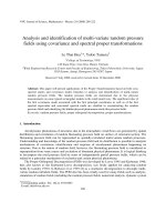
Fig. 1. Wind tunnel configuration, experimental set-ups and experimental models.
Flow around models due to interaction between ongoing flow and model section is usually known
as the bluff body flow, which characterized by formation of separated and reattached flows with
separation bubble and formation of vortex shedding as well. It can be predicted from the past
knowledge that model B/D=1 is favorable for formation of Karman vortex shedding, where model
φ

Turntable
Honeycomb

Small test section
Large test section
Motor
Mesh
Wind
1
st
Entrance Cone

2
nd
Entrance Cone
Adjustable wall
Grid Model
Support and loadcell

2000
4200
Open-circuit wind tunnel
Fan

Silencer

14000

1850
1300
6550

1300

3000
1800
Wind Wind Splitter Plate (S.P)
B/D=1 B/D=1 with S.P
B/D=5
Wind
po1…
po19
po10
po1…
po1…
po10
L.T. Hoa, Yukio Tamura / VNU Journal of Science, Mathematics - Physics 24 (2008) 209-222
214

B/D=5 is typical for formation of separated and reattached flows on model surface. The splitter plate
was added to model B/D=1 to suppress effect of Karman vortex.

Fig. 2. Bluff body flow patterns around experimental models.
The bluff body flow patterns around three experimental models can be predicted as shown above
in Figure 2 (bluff-body flows on one surface are drawn).
4. Surface pressure distribution and bluff body flow pattern
Mean and root-mean-square fluctuating pressure coefficients have been normalized by dynamic
pressure component from measured unsteady pressure data as follows:

(
)
2
,
5.0 UpC

meanp
ρ
=
;
(
)
2
,
5.0 UC
prmsp
ρσ
=
(15)
where
2
5.0 U
ρ
: dynamic pressure;
p
: mean pressure;
p
σ
: standard deviation of unsteady pressure.
Fig. 3. Normalized fluctuating pressure distribution on chordwise positions.
Figure 3 shows the chordwise distributions of normalized fluctuating pressures on models at
three turbulent flow conditions. As can be seen that the fluctuating pressure distributes steadily on
whole surface of models B/D=1 but distributes dominantly on the leading region of the model B/D=5.
The fluctuating pressures, furthermore, reduce with respect to decrease of intensities of turbulence.

1 2 3 4 5 6 7 8 9 10
0
0.05
0.1
0.15
0.2
0.25
0.3
0.35
0.4
0.45
0.5
Positions
C
p,rm s
I
u
=11.46% I
w
=11.23%
I
u
=10.54% I
w
=9.28%
I
u
=9.52% I
w
=6.65%

1 2 3 4 5 6 7 8 9 10
0
0.05
0.1
0.15
0.2
0.25
0.3
0.35
0.4
Positions
C
p,rm s
I
u
=11.46% I
w
=11.23%
I
u
=10.54% I
w
=9.28%
I
u
=9.52% I
w
=6.65%
1 2 3 4 5 6 7 8 9 10 11 12 13 14 15 16 17 18 19
0

0.05
0.1
0.15
0.2
0.25
0.3
0.35
0.4
Positions
Cp ,rms
Normalized fluctuating pressure
I
u
=11.46% I
w
=11.23%
I
u
=10.54% I
w
=9.28%
I
u
=9.52% I
w
=6.65%
Wind
B/D=1 B/D=1 with S.P
B/D=5

Wind
Wind
U=9m/s
U=6m/s U=3m/s
L.T. Hoa, Yukio Tamura / VNU Journal of Science, Mathematics - Physics 24 (2008) 209-222
215
Fig. 4. Power spectra of fluctuating pressures at some chordwise positions.
Figure 4 indicates power spectra of the fluctuating pressures at some chordwise positions with
three models and turbulent conditions. As can be seen with the model B/D=1 (without splitter plate)
that peaked frequencies are observed at 4.15Hz, 8.79Hz and 12.94Hz respective to the three turbulent
flows. It is explained that the Karman vortex formed and shed at the wake of model. Shedding
frequency depends on the Strouhal number (S
t
) of cross section, moreover, the Strouhal number can be
determined St=0.1285. In case B/D=1 with splitter plate, no peaked frequency is observed, it also
means that no Karman vortex occurred and the splitter plate has suppressed effect of the Karman
vortex. In case of the model B/D=5, spectral peaks are also observed at frequencies 1.22Hz and
2.44Hz (U=3m/s); at 2.44Hz, 4.88Hz, 7.32Hz (case 2); at 3.42Hz and 6.84Hz (case 3). It is predicted
that the bluff body flow is separated and reattached one. Reattachment points are at roughly positions
6, 7, 8 with respect to an increase of mean velocities. It is supposed that the observed spectral peaks
are induced by rolled-up vortices shed away at reattachment points toward trailing edge. This agrees
well with findings presented in the literatures of Hiller and Cherry, 1981 and Cherry et al.,1984 which
were proposed empirical formula to estimate frequency of rolled-up vortices shedding at reattachment
point depending on mean velocity and length of separation bubble.
B/D=1
10
-1
10
0
10

1
10
2
10
-3
10
-2
10
-1
10
0
10
1
10
2
10
3
10
4
Frequency n(Hz)
PSD
po.1
po.3
po.5
po.7
po.9
U=3m/s
4.15Hz 1.22Hz
10
-1

10
0
10
1
10
2
10
-1
10
0
10
1
10
2
10
3
10
4
Frequency n(Hz)
PSD
po1
po3
po5
po7
po9
8.79Hz
U=6m/s
10
-1
10

0
10
1
10
2
10
0
10
1
10
2
10
3
10
4
10
5
Frequency n(Hz)
PSD
po1
po3
po5
po7
po9
U=9m/s
12.94Hz
10
-1
10
0

10
1
10
2
10
-3
10
-2
10
-1
10
0
10
1
10
2
10
3
Frequency n(Hz)
PSD
po1
po3
po5
po7
po9
U=3m/s
1.22Hz
B/D=1 (with S.P)
10
-1

10
0
10
1
10
2
10
-1
10
0
10
1
10
2
10
3
10
4
Frequency n(Hz)
PSD
po1
po3
po5
po7
po9
U=6m/s
10
-1
10
0

10
1
10
2
10
0
10
1
10
2
10
3
10
4
Frequency n(Hz)
PSD
po1
po3
po5
po7
po9
U=9m/s
10
-1
10
0
10
1
10
2

10
-7
10
-6
10
-5
10
-4
10
-3
10
-2
10
-1
Frequency (Hz)
PSD of pressure(1/Hz)
po.1
po.2
po.5
po.6
po.9
po.10
po.18
po.19
U=3m/s
1.22Hz
2.44Hz
10
-1
10

0
10
1
10
2
10
-7
10
-6
10
-5
10
-4
10
-3
10
-2
10
-1
Frequency (Hz)
PSD of pressure(1/Hz)
po.1
po.2
po.5
po.6
po.9
po.10
po.18
po.19
U=6m/s

2.44Hz
4.88Hz
7.32Hz
10
-1
10
0
10
1
10
2
10
-7
10
-6
10
-5
10
-4
10
-3
10
-2
10
-1
Frequency (Hz)
PSD of pressure(1/Hz)
po.1
po.2
po.5

po.6
po.9
po.10
po.18
po.19
U=9m/s
3.42Hz
6.84Hz
B/D=5
L.T. Hoa, Yukio Tamura / VNU Journal of Science, Mathematics - Physics 24 (2008) 209-222
216

5. Results and discussion
5.1. Analysis on covariance matrix branch
Eigenvalues and eigenvectors (covariance pressure modes) have been determined from covariance
matrix of chordwise fluctuating pressures. Figure 5 shows first four covariance modes along
chordwise positions at the flow case 1 of U=3m/s (two other cases are similar and not be interpreted
here for sake of brevity). It is noted that all first covariance modes look alike to the fluctuating
pressure distributions.
Energy contribution of the lowest covariance modes, estimated following Eq.(9) is given in Table
1. Obviously, the first covariance mode contributes dominantly to system, energy contribution here
calculates following the Eq.(9). The first covariance modes contribute 76.92%, 65.29%, 43.77% to
total energy at the flow case 1 corresponding to models B/D=1 with and without the splitter plate and
model B/D=5, respectively in the flow case 1. If first two covariance modes are taken into account, the
energy of these modes holds up to 90.19%, 86.26%, 65.79% of total energy. It is noted that the first
covariance mode in the model B/D=5 holds energy contribution of only 43.77% to compare with that
of 76.92%, 65.29% in the other models of B/D=1. This can be explained due to complexity of bluff
body flow around the model B/D=5 to reduce a role of the first covariance mode.

Fig. 5. First four covariance pressure modes of experimental models.
Table 1. Energy contribution of covariance pressure modes (%)
Mode B/D=1 B/D=1 with S.P B/D=5
3m/s 6m/s 9m/s 3m/s 6m/s 9m/s 3m/s 6m/s 9m/s
1
76.92 77.46 75.36 65.29 62.79 63.30 43.77 44.86 65.9
2
13.27 13.25 14.41 20.97 22.61 22.08 22.02 23.14 13.29
3
4.69 4.23 4.62 6.14 6.29 6.10 15.18 15.14 9.48
4
2.87 2.86 3.17 4.04 4.32 4.41 5.98 5.68 3.40
5
1.27 1.32 1.45 1.99 2.28 2.45 4.76 4.11 2.79
1 2 3 4 5 6 7 8 9 10 11 12 13 14 15 16 17 18 19
-0.8
-0.6
-0.4
-0.2
0

0.2
0.4
0.6
Positions
Modes
mode 1
mode 2
mode 3
mode 4
1 2 3 4 5 6 7 8 9 10
-0.8
-0.6
-0.4
-0.2
0
0.2
0.4
0.6
0.8
Positions
Modes
mode 1
mode 2
mode 3
mode 4
1 2 3 4 5 6 7 8 9 10
-1
-0.75
-0.5
-0.25

0
0.25
0.5
0.75
1
Positions
Modes
mode 1
mode 2
mode 3
mode 4
B/D=1 B/D=1 with S.P B/D=5
L.T. Hoa, Yukio Tamura / VNU Journal of Science, Mathematics - Physics 24 (2008) 209-222
217
Fig. 6. First four principal coordinates and their power spectral densities.
Uncorrelated principal coordinates associated with the covariance pressure modes has been
calculated from the measured pressure data, as first four principal coordinates of three models at the
flow case 1 and their corresponding power spectra are shown in Figure 6. It is noteworthy that first
coordinates not only dominate in the power spectrum but contain frequency characteristics of
the random pressure field, whereas the other coordinates do not contain these frequencies. Thus, the
first covariance pressure modes and associated principal coordinate will play very important role in the
identification of random pressure field due to their dominant energy contribution and frequency
containing of hidden physical events of system.
5.2. Analysis on spectral matrix branch
Frequency dependant eigenvalues and eigenvectors (spectral modes) are obtained from the cross
spectral matrix of the observed pressure field. Figure 7 shows first five spectral eigenvalues on
frequency band 0÷50Hz at the flow case 1 (U=3m/s). As can be seen from Figure 7, all first spectral
eigenvalues from three models exhibit much dominantly than others, especially theses first
eigenvalues also contain all frequency peaks of the pressure field, whereas others do not hold theses
peaks. This finding means in these investigations that the first spectral mode can represent for hidden

characteristics of the pressure fields, concretely here the first mode contains frequency of any physical
phenomenon happening on models.
Energy contributions of spectral pressure modes are expressed in Table 2. Similar to the
covariance pressure modes, the first spectral pressure modes contain dominantly the system energy of
0 5 10
-20
-10
0
10
20
Time (s)
Coordinate 1
0 5 10
-20
-10
0
10
20
Time (s)
Coordinate 2
0 5 10
-20
-10
0
10
20
Time (s)
Coordinate 3
0 5 10
-20

-10
0
10
20
Time (s)
Coordinate 4
0 5 10
-10
-5
0
5
10
Time (s)
Coordinate 1
0 5 10
-10
-5
0
5
10
Time (s)
Coordinate 2
0 5 10
-10
-5
0
5
10
Time (s)
Coordinate 3

0 5 10
-10
-5
0
5
10
Time (s)
Coordinate 4
0 5 10
-10
-5
0
5
10
Time (s)
Coordinate 1
0 5 10
-10
-5
0
5
10
Time (s)
Coordinate 2
0 5 10
-10
-5
0
5
10

Time (s)
Coordinate 3
0 5 10
-10
-5
0
5
10
Time (s)
Coordinate 4
B/D=1 B/D=1 with S.P B/D=5
10
-1
10
0
10
1
10
2
10
-6
10
-5
10
-4
10
-3
10
-2
10

-1
10
0
10
1
Frequency (Hz)
PSD
coordinate 1
coordinate 2
coordinate 3
coordinate 4
10
-1
10
0
10
1
10
2
10
-6
10
-5
10
-4
10
-3
10
-2
10

-1
10
0
10
1
Frequency (Hz)
PSD
Principal coordinates
coordinate 1
coordinate 2
coordinate 3
coordinate 4
10
-1
10
0
10
1
10
2
10
-6
10
-5
10
-4
10
-3
10
-2

10
-1
10
0
10
1
Frequency (Hz)
PSD
coordinate 1
coordinate 2
coordinate 3
coordinate 4
4.15Hz 1.22Hz
L.T. Hoa, Yukio Tamura / VNU Journal of Science, Mathematics - Physics 24 (2008) 209-222
218

the unsteady pressure fields, for example, the first pressure mode contribute 86.04%, 81.30%, 74.77%,
respectively to the three experimental models at the flow case 1 (U=3m/s). In the cases of two modes
combined, the first two pressure modes contribute almost 94.12%, 91.45%, 87.45% on the total
energy, respectively. It is also the same as the covariance matrix branch that the first spectral mode
contributes 74.77% to the energy in the model B/D=5, whereas it holds 86.04% and 81.30% in two
other models of B/D=1. This might be also due to an influence of separating and reattachment flow on
the modal surface, moreover, it might suggest that the more complicate the random pressure fields
exhibit the less important the first mode contributes.

Fig. 7. First five spectral eigenvalues of experimental models.
Table 2. Energy contribution of spectral pressure modes (%)
Mode B/D=1 B/D=1 with S.P B/D=5
3m/s 6m/s 9m/s 3m/s 6m/s 9m/s 3m/s 6m/s 9m/s
1
86.04 85.84 83.02 81.30 77.48 77.88 74.77 73.59 83.93
2
8.08 8.08 9.92 10.15 12.36 11.98 12.68 14.03 7.69
3
3.28 3.20 3.68 4.44 5.14 5.00 5.68 5.56 3.57
4
1.40 1.62 1.94 2.05 2.63 2.70 2.75 2.86 1.86
5
0.64 0.72 0.81 1.09 1.28 1.34 1.44 1.45 1.06

In comparison on the energy contribution between the covariance modes and the spectral ones, as
can be seen from Tables 1 and 2 that the first spectral mode contributes higher than the first covariance
one. Concretely, the first spectral mode holds 94.12%, 91.45%, 87.45% comparing with 76.92%,
65.29%, 43.77% of the first covariance one in the three models of B/D=1, B/D=1 with splitter plate
and B/D=5, respectively at the flow case 1 (U=3m/s), similarly, 83.02%, 77.88%, 83.93% to compare
with 75.36%, 63.3%, 65.9% at flow case 3 (U=9m/s). It might suggest that the first spectral mode
exhibits better than the first covariance one in the analysis, synthesis and identification of the random
pressure fields.

10
-1
10
0
10
1
10
2
10
-5
10
-4
10
-3
10
-2
10
-1
10
0
10
1
Frequency (Hz)
Spectral eigenvalues
λ
1
λ
2
λ
3

λ
4
λ
5
10
-1
10
0
10
1
10
2
10
-5
10
-4
10
-3
10
-2
10
-1
10
0
10
1
Frequency (Hz)
Spectral eigenvalues
λ
1

λ
2
λ
3
λ
4
λ
5
10
-1
10
0
10
1
10
2
10
-4
10
-3
10
-2
10
-1
10
0
10
1
Frequency (Hz)
Spectral eigenvalues

λ
1
λ
2
λ
3
λ
4
λ
5
B/D=1 B/D=1 with S.P B/D=5
L.T. Hoa, Yukio Tamura / VNU Journal of Science, Mathematics - Physics 24 (2008) 209-222
219

Fig. 8. First three spectral pressure modes of experimental models.
The first three spectral pressure modes of the chordwise fluctuating pressure fields of experimental
models in the flow case 1 are shown at Figure 8 in frequency band 0-50Hz. It seems that more
investigations must be needed to clarify the physical meaning of the spectral pressure modes as well as
the linkage between the pressure modes and hidden events of the unsteady pressure fields.
6. Synthesis and identification of random pressure field
Firstly, effects of basic and cumulative covariance modes on the synthesis of the unsteady pressure
fields, as well as role of the first covariance mode on the identification of these pressure fields will be
verified and investigated. Figures 9 and Figure 10 show the pressure synthesis and the spectral
pressure one at referred position 5 using individually basic covariance modes (1
st
mode, 2
nd
mode, 3
rd

mode and 4
th
mode), whereas Figure 11 indicated the cumulative covariance modes (1
st
mode and first
2 modes), respectively with verifying spectral synthesis of the covariance modes to original time series
of pressures (as target), only position 5 and flow case 1 presented due to brevity.
B/D=
5

B/D=1

B/D=1 with S.P

L.T. Hoa, Yukio Tamura / VNU Journal of Science, Mathematics - Physics 24 (2008) 209-222
220












Fig. 9. Effect of basic covariance modes on pressure synthesis at referred position 5.

Fig. 10. Effect of basic covariance modes on spectral pressure synthesis at referred position 5.
Fig. 11. Effect of cumulative covariance modes on pressure synthesis at referred position 5.
0 500 10 00 1500 200 0
-8
-6
-4
-2
0
2
4
6
8
A m pli tu d e
Position 5
target
1
st
mode

0 500 10 00 1500 200 0
-8
-6
-4
-2
0
2
4
6
8
A m pli tu d e
Position 5
target
2
nd
mode
0 500 10 00 1500 200 0
-8
-6
-4
-2
0
2
4
6
8
Time (ms)
A m plit ud e
Position 5
target

2
rd
mode
0 500 10 00 1500 200 0
-8
-6
-4
-2
0
2
4
6
8
Time (ms)
A m plit ud e
Position 5
target
4
st
modes
0 500 10 00 1500 200 0
-6
-4
-2
0
2
4
6
A m pli tu d e
Position 5

target
1
st
mode
0 500 10 00 1500 200 0
-6
-4
-2
0
2
4
6
A m pli tu d e
Position 5
target
2
nd
mode
0 500 10 00 1500 200 0
-6
-4
-2
0
2
4
6
Time (ms)
A m plit ud e
Position 5
target

2
rd
mode
0 500 10 00 1500 200 0
-6
-4
-2
0
2
4
6
Time (ms)
A m plit ud e
Position 5
target
4
st
modes
0 500 10 00 1500 200 0
-6
-4
-2
0
2
4
6
A m pli tu d e
Position 5
target
1

st
mode
0 500 10 00 1500 200 0
-6
-4
-2
0
2
4
6
A m pli tu d e
Position 5
target
2
nd
mode
0 500 10 00 1500 200 0
-6
-4
-2
0
2
4
6
Time (ms)
A m plit ud e
Position 5
target
2
rd

mode
0 500 10 00 1500 200 0
-6
-4
-2
0
2
4
6
Time (ms)
A m plit ud e
Position 5
target
4
st
modes
B/D=1

B/D=1

with

S
P

B/D=5

10
-1
10

0
10
1
10
2
10
-5
10
-3
10
0
10
2
P S D
Position 5
target
1
st
mode
10
-1
10
0
10
1
10
2
10
-5
10

-3
10
0
10
2
P S D
Position 5
target
2
nd
mode
10
-1
10
0
10
1
10
2
10
-5
10
-3
10
0
10
2
Frequency (Hz)
P S D
Position 5

target
3
rd
mode
10
-1
10
0
10
1
10
2
10
-7
10
-5
10
-3
10
0
10
2
Frequency (Hz)
P S D
Position 5
target
4
st
mode
10

-1
10
0
10
1
10
2
10
-5
10
-3
10
0
10
1
P S D
Position 5
target
1
st
mode
10
-1
10
0
10
1
10
2
10

-5
10
-3
10
0
10
1
P S D
Position 5
target
2
nd
mode
10
-1
10
0
10
1
10
2
10
-5
10
-3
10
0
10
1
Frequency (Hz)

P S D
Position 5
target
3
rd
mode
10
-1
10
0
10
1
10
2
10
-7
10
-5
10
-3
10
0
10
1
Frequency (Hz)
P S D
Position 5
target
4
st

mode
10
-1
10
0
10
1
10
2
10
-5
10
-3
10
0
10
1
P S D
Position 5
target
1
st
mode
10
-1
10
0
10
1
10

2
10
-5
10
-3
10
0
10
1
P S D
Position 5
target
2
nd
mode
10
-1
10
0
10
1
10
2
10
-5
10
-3
10
0
10

1
Frequency (Hz)
P S D
Position 5
target
3
rd
mode
10
-1
10
0
10
1
10
2
10
-5
10
-3
10
0
10
1
Frequency (Hz)
P S D
Position 5
target
4
st

mode
0 500 1000 1500 2000
-8
-6
-4
-2
0
2
4
6
8
A m plit ude
Position 5
Time (ms)
target
1
st
mo de
0 500 1000 1500 2000
-8
-6
-4
-2
0
2
4
6
8
A m plit ude
Position 5

Time (ms)
target
1
st
to 2
nd
mo des
10
-1
10
0
10
1
10
2
10
-5
10
-3
10
0
10
2
P S D
Frequency (Hz)
target
1
st
mode
10

-1
10
0
10
1
10
2
10
-5
10
-3
10
0
10
2
P S D
Frequency (Hz)
target
1
st
to 2
nd
mo des
0 500 1000 1500 2000
-8
-6
-4
-2
0
2

4
6
8
A mp l itu d e
Time (ms)
Position 5
0 500 1000 1500 2000
-8
-6
-4
-2
0
2
4
6
8
A mp l itu d e
Time (ms)
Position 5
10
-1
10
0
10
1
10
2
10
-5
10

-3
10
0
P SD
Frequency (Hz)
10
-1
10
0
10
1
10
2
10
-5
10
-3
10
0
P SD
Frequency (Hz)
target
1
st
mo de
target
1
st
to 2
nd

mo des
target
1
st
mode
target
1
st
to 2
nd
mo des
0 500 1000 1500 2000
-8
-6
-4
-2
0
2
4
6
8
A mp l itu d e
Position 5
Time (ms)
0 500 1000 1500 2000
-8
-6
-4
-2
0

2
4
6
8
A mp l itu d e
Position 5
Time (ms)
10
-1
10
0
10
1
10
2
10
-5
10
-3
10
0
P SD
Frequency (Hz)
10
-1
10
0
10
1
10

2
10
-5
10
-3
10
0
P SD
Frequency (Hz)
target
1
st
mode
target
1
st
to 2
nd
modes
target
1
st
mode
target
1
st
to 2
nd
mo des
B/D=1

B/D=1 with S.P

B/D=5

L.T. Hoa, Yukio Tamura / VNU Journal of Science, Mathematics - Physics 24 (2008) 209-222
221
As can be seen from Figure 9, Figure 10 that reconstructed pressure time series using the first
covariance pressure mode is similar to the original pressure, especially its containing of frequency
peaks can be used to identify hidden characteristics and physical phenomena of the original pressure.
In comparison, reconstructed pressure portions using 2
nd
mode, 3
rd
mode, 4
th
mode are minor
contributions to the original pressure, and these pressure portions do not contain the frequency peaks
in the original pressure. Reconstructed pressure using the first mode, moreover, seems to be good
agreement to the original pressure at low frequency range between 0-10Hz in models B/D=1, but it is
notable in spectral difference between reconstructed pressure and original one at high frequency range
in models B/D=1 and all frequency range (excepting at frequency peaks) in model B/D=5. It is argued
that the first mode is enough for the reconstructed pressure at the low frequencies in models B/D=1,
but more cumulative modes may be needed for the reconstructed pressure at the high frequencies. In
the model B/D=5, moreover, the first mode can be used to identify the field, but it is not enough to
reconstruct the original pressure, then more modes should be needed for the pressure reconstruction
due to more complicate distribution of pressure field.
In the Figure 11, reconstructed pressure using the first mode and cumulative two modes and their
PSD are presented, it can be seen that only the first mode is enough to reconstruct the original pressure
in models B/D=1, the cumulative two modes are enough in model B/D=5.

Fig. 12. Effects of basic and cumulative spectral modes on spectral synthesis of pressure position 5.
Secondly, effects of basic and cumulative spectral pressure modes on the synthesis of the unsteady
pressure fields, as well as role of the first spectral mode on the identification of these pressure fields
10
-1
10
0
10
1
10
2
10
-8
10
-7
10
-6
10
-5
10
-4
10
-3
10
-2
10
-1
10
0
Frequency (Hz)

P SD
Position 5
target
1
st
mode
2
nd
mode
3
rd
mode
4
th
mode
10
-1
10
0
10
1
10
2
10
-6
10
-5
10
-4
10

-3
10
-2
10
-1
10
0
Frequency (Hz)
P SD
Position 5
target
1
st
mode
1
st
to 2
nd
modes
10
-1
10
0
10
1
10
2
10
-8
10

-7
10
-6
10
-5
10
-4
10
-3
10
-2
10
-1
10
0
Frequency (Hz)
P SD
Position 5
target
1
st
mode
2
nd
mode
3
rd
mode
4
th

mode
10
-1
10
0
10
1
10
2
10
-6
10
-5
10
-4
10
-3
10
-2
10
-1
10
0
Frequency (Hz)
P SD
Position 5
target
1
st
mode

1
st
to 2
nd
modes
10
-1
10
0
10
1
10
2
10
-8
10
-7
10
-6
10
-5
10
-4
10
-3
10
-2
10
-1
10

0
Frequency (Hz)
P SD
Position 5
target
1
st
mode
2
nd
mode
3
rd
mode
4
th
mode
10
-1
10
0
10
1
10
2
10
-5
10
-4
10

-3
10
-2
10
-1
10
0
Frequency (Hz)
P SD
Position 5
target
1
st
mode
1
st
to 2
nd
modes
B/D=1

B/D=1 with S.P

B/D=5

L.T. Hoa, Yukio Tamura / VNU Journal of Science, Mathematics - Physics 24 (2008) 209-222
222

will be investigated. Figure 12 above shows the effects of individual and cumulative spectral modes on
the synthesis of auto spectra density of the pressure fields, here pressure at referred position 5 in the

flow case 1 of U=3m/s is used for demonstration. As can be seen in upper row that the first spectral
mode only is accuracy enough to reconstruct and identify the original pressure in all three
experimental models and whole frequency range. There are also good agreements between spectrum
of the original pressure and reconstructed spectrum using the first mode and cumulative two modes.
7. Conclusion
Analysis and identification of the unsteady pressure fields measured on some typical rectangular
sections using both the Covariance Proper Transformation in the time domain and the Spectral Proper
Transformation in the frequency domain have been presented in this paper. So-called the covariance
pressure modes and the spectral pressure ones have been orthogonally decomposed from the
covariance matrix and the spectral one as the comprehensive descriptions of the unsteady pressure
fields. Some conclusions can be pointed out as follows:
The first covariance pressure mode and the first spectral mode as well play very important role in
analysis, synthesis and identification of the unsteady pressure fields. It contributes dominantly the
system energy of the pressure fields as well as contains certain frequency peaks of possibly physical
phenomena hidden in these pressure fields. Moreover, it seems that the first spectral pressure mode
exhibits better than the first covariance one in the analysis, synthesis and identification of the unsteady
pressure fields
In low frequency range, only the first mode (either the covariance pressure mode or the spectral
pressure one) can reconstruct the unsteady pressure fields with enough accuracy, whereas more
cumulative modes should be needed to reconstruct the unsteady pressure field in the cases of the high
frequency range and of the complicated pressure distributions and flows as well. In other words, the
more complicated the pressure field distributes and the bluff body flow behaviors, the less important the
first mode contributes and the more cumulative modes are needed to reconstruct the pressure fields.
References
[1] J.L. Lumley, Stochastic tools in turbulence, Academic Press 1970.
[2] G. Berkooz, P. Holmes, J.L. Lumley, The proper orthogonal decomposition in the analysis of turbulent flows, Annu. Rev.
Fluid Mech. 25 (1992) 539.
[3] B. Bienkiewicz, Y. Tamura, H.J. Ham, H. Ueda, K. Hibi, Proper orthogonal decomposition and construction of multi-
channel roof pressure, J. of Wind Eng. Ind. Aerodyn 54-55 (1995) 369.
[4] J.D. Holmes, R. Sankaran, K.C.S. Kwok, M.J. Syme, Eigenvector modes of fluctuating pressures on low-rise building

models, J. of Wind Eng Ind. Aerodyn 69-71(1997) 697.
[5] S.H. Jeong, B. Bienkiewicz, H.J. Ham, Proper orthogonal decomposition of building wind pressure specified at non-
uniform distributed pressure taps, J. of Wind Eng.Ind. Aerodyn 87 (1997) 1.
[6] H. Kikuchi, Y. Tamura, H. Ueda, K. Hibi, Dynamic wind pressure acting on a tall building model - Proper orthogonal
decomposition, J. of Wind Eng. Ind. Aerodyn 69-71 (1997) 631.
[7] Y. Tamura, H. Ueda, H. Kikuchi, K. Hibi, S. Suganuma, B. Bienkiewicz, Proper orthogonal decomposition study of
approach wind-building pressure correlation, J. of Wind Eng. Ind. Aerodyn 72 (1997) 421.
[8] Y. Tamura, S. Suganuma, H. Kikuchi, K. Hibi, Proper orthogonal decomposition of random wind pressure field, J. of
Fluids and Structures 13 (1999) 1069.
[9] E.T. De Grenet, F. Ricciardelli, Spectral proper transformation of wind pressure fluctuation: application to a square
cylinder and a bridge deck, J. of Wind Eng. Ind. Aerodyn 92 (2004) 1281.