handbook for electrical engineers hu (2)

SECTION 3
MEASUREMENTS AND
INSTRUMENTS
*
Gerald J. Fitzpatsick
Project Leader, Advanced Power System Measurements
National Institute of Standard and Technology
CONTENTS
3.1 ELECTRIC AND MAGNETIC MEASUREMENTS . . . . . . . .3-1
3.1.1 General . . . . . . . . . . . . . . . . . . . . . . . . . . . . . . . . . . .3-1
3.1.2 Detectors and Galvanometers . . . . . . . . . . . . . . . . . . .3-4
3.1.3 Continuous EMF Measurements . . . . . . . . . . . . . . . .3-9
3.1.4 Continuous Current Measurements . . . . . . . . . . . . . .3-13
3.1.5 Analog Instruments . . . . . . . . . . . . . . . . . . . . . . . . .3-14
3.1.6 DC to AC Transfer . . . . . . . . . . . . . . . . . . . . . . . . . .3-16
3.1.7 Digital Instruments . . . . . . . . . . . . . . . . . . . . . . . . . .3-16
3.1.8 Instrument Transformers . . . . . . . . . . . . . . . . . . . . .3-18
3.1.9 Power Measurement . . . . . . . . . . . . . . . . . . . . . . . . .3-19
3.1.10 Power-Factor Measurement . . . . . . . . . . . . . . . . . . .3-21
3.1.11 Energy Measurements . . . . . . . . . . . . . . . . . . . . . . .3-22
3.1.12 Electrical Recording Instruments . . . . . . . . . . . . . . .3-27
3.1.13 Resistance Measurements . . . . . . . . . . . . . . . . . . . . .3-29
3.1.14 Inductance Measurements . . . . . . . . . . . . . . . . . . . .3-38
3.1.15 Capacitance Measurements . . . . . . . . . . . . . . . . . . .3-41
3.1.16 Inductive Dividers . . . . . . . . . . . . . . . . . . . . . . . . . .3-45
3.1.17 Waveform Measurements . . . . . . . . . . . . . . . . . . . . .3-46
3.1.18 Frequency Measurements . . . . . . . . . . . . . . . . . . . . .3-46
3.1.19 Slip Measurements . . . . . . . . . . . . . . . . . . . . . . . . . .3-48
3.1.20 Magnetic Measurements . . . . . . . . . . . . . . . . . . . . . .3-48
3.2 MECHANICAL POWER MEASUREMENTS . . . . . . . . . . .3-51
3.2.1 Torque Measurements . . . . . . . . . . . . . . . . . . . . . . .3-51

3.2.2 Speed Measurements . . . . . . . . . . . . . . . . . . . . . . . .3-51
3.3 TEMPERATURE MEASUREMENT . . . . . . . . . . . . . . . . . .3-52
3.4 ELECTRICAL MEASUREMENT OF NONELECTRICAL
QUANTITIES . . . . . . . . . . . . . . . . . . . . . . . . . . . . . . . . . . . .3-56
3.5 TELEMETERING . . . . . . . . . . . . . . . . . . . . . . . . . . . . . . . . .3-61
3.6 MEASUREMENT ERRORS . . . . . . . . . . . . . . . . . . . . . . . . .3-64
BIBLIOGRAPHY . . . . . . . . . . . . . . . . . . . . . . . . . . . . . . . . . . . . .3-66
3.1 ELECTRIC AND MAGNETIC MEASUREMENTS
3.1.1 General
Measurement of a quantity consists either of its comparison with a unit quantity of the same kind or
of its determination as a function of quantities of different kinds whose units are related to it by
known physical laws. An example of the first kind of measurement is the evaluation of a resistance
3-1
*Grateful acknowledgement is given to Norman Belecki, George Burns, Forest Harris, and B.W. Mangum for most of the
material in this section.
Beaty_Sec03.qxd 17/7/06 8:26 PM Page 3-1
Downloaded from Digital Engineering Library @ McGraw-Hill (www.digitalengineeringlibrary.com)
Copyright © 2006 The McGraw-Hill Companies. All rights reserved.
Any use is subject to the Terms of Use as given at the website.
Source: STANDARD HANDBOOK FOR ELECTRICAL ENGINEERS
3-2 SECTION THREE
(in ohms) with a Wheatstone bridge in terms of a calibrated resistance and a ratio. An example of the
second kind is the calibration of the scale of a wattmeter (in watts) as the product of current (in
amperes) in its field coils and the potential difference (in volts) impressed on its potential circuit.
The units used in electrical measurements are related to the metric system of mechanical units in
such a way that the electrical units of power and energy are identical with the corresponding mechan-
ical units. In 1960, the name Système International (abbreviated SI), now in use throughout the
world, was assigned to the system based on the meter-kilogram-second-ampere (abbreviated mksa).
The mksa units are identical in value with the practical units—volt, ampere, ohm, coulomb, farad,
henry—used by engineers. Certain prefixes have been adopted internationally to indicate decimal

multiples and fractions of the basic units.
A reference standard is a concrete representation of a unit or of some fraction or multiple of it
having an assigned value which serves as a measurement base. Its assignment should be traceable
through a chain of measurements to the National Reference Standard maintained by the National
Institute of Standards and Technology (NIST). Standard cells and certain fixed resistors, capacitors,
and inductors of high quality are used as reference standards.
The National Reference Standards maintained by the NIST comprise the legal base for measure-
ments in the United States. Other nations have similar laboratories to maintain the standards which
serve as their measurement base. An international bureau—Bureau International des Poids et Mesures
(abbreviated BIPM) in Sèvres, France—also maintains reference standards and compares standards
from the various national laboratories to detect and reconcile any differences that might develop
between the as-maintained units of different countries.
At NIST, the reference standard of resistance is a group of 1-Ω resistors, fully annealed and
mounted strain-free out of contact with the air, in sealed containers. The reference standard of capac-
itance is a group of 10-pF fused-silica-dielectric capacitors whose values are assigned in terms of the
calculable capacitor used in the ohm determination. The reference standard of voltage is a group of
standard cells continuously maintained at a constant temperature.
The “absolute” experiments from which the value of an electrical unit is derived are measurements
in which the electrical unit is related directly to appropriate mechanical units. In recent ohm determi-
nations, the value of a capacitor of special design was calculated from its measured dimensions, and
its impedance at a known frequency was compared with the resistance of a special resistor. Thus, the
ohm was assigned in terms of length and time. The as-maintained ohm is believed to be within 1 ppm
of the defined SI unit. Recent ampere determinations, used to assign the volt in terms of current and
resistance, derived the ampere by measuring the force between current-carrying coils of a mutual
inductor of special construction whose value was calculated from its measured dimensions. The volt-
age drop of this current in a known resistor was used to assign the emf of the standard cells which
maintain the volt. The stated uncertainty of these ampere determinations ranges from 4 to 7 ppm, and
the departure of value of the “legal” volt from the defined SI unit carries the same uncertainty. Since
1972, the assigned emf of the standard cells in the reference group which maintains the legal volt is
monitored (and reassigned as necessary) in terms of atomic constants (the ratio of Planck’s constant

to electron charge) and a microwave frequency by an ac Josephson experiment in which their voltage
is measured with respect to the voltage developed across the barrier junction between two supercon-
ductors irradiated by microwave energy and biased with a direct current. This experiment appears to
be repeatable within 0.1 ppm. It should be noted that while the Josephson experiment may be used to
maintain the legal volt at a constant level, it is not used to define the SI unit.
Precision—a measure of the spread of repeated determinations of a particular quantity—depends
on various factors. Among these are the resolution of the method used, variations in ambient condi-
tions (such as temperature and humidity) that may influence the value of the quantity or of the ref-
erence standard, instability of some element of the measuring system, and many others. In the
National Laboratory of the National Institute of Standards and Technology, where every precaution
is taken to obtain the best possible value, intercomparisons may have a precision of a few parts in
10
7
. In commercial laboratories, where the objective is to obtain results that are reliable but only to
the extent justified by engineering or other requirements, precision ranges from this figure to a part
in 10
3
or more, depending on circumstances. For commercial measurements such as the sale of elec-
trical energy, where the cost of measurement is a critical factor, a precision of 1 or 2% is considered
acceptable in some jurisdictions.
Beaty_Sec03.qxd 17/7/06 8:26 PM Page 3-2
Downloaded from Digital Engineering Library @ McGraw-Hill (www.digitalengineeringlibrary.com)
Copyright © 2006 The McGraw-Hill Companies. All rights reserved.
Any use is subject to the Terms of Use as given at the website.
MEASUREMENTS AND INSTRUMENTS*
MEASUREMENTS AND INSTRUMENTS 3-3
The use of digital instruments occasionally creates a problem in the evaluation of precision, that
is, all results of a repeated measurement may be identical due to the combination of limited resolu-
tion and quantized nature of the data. In these cases, the least count and sensitivity of the instru-
mentation must be taken into account in determining precision.

Accuracy—a statement of the limits which bound the departure of a measured value from the true
value of a quantity—includes the imprecision of the measurement, together with all the accumulated
errors in the measurement chain extending downward from the basic reference standards to the spe-
cific measurement in question. In engineering measurement practice, accuracies are generally stated
in terms of the values assigned to the National Reference Standards—the legal units. It is only rarely
that one needs also to state accuracy in terms of the defined SI unit by taking into account the uncer-
tainty in the assignment of the National Reference Standard.
General precautions should be observed in electrical measurements, and sources of error should
be avoided, as detailed below:
1. The accuracy limits of the instruments, standards, and methods used should be known so that
appropriate choice of these measuring elements may be made. It should be noted that instrument
accuracy classes state the “initial” accuracy. Operation of an instrument, with energy applied
over a prolonged period, may cause errors due to elastic fatigue of control springs or resistance
changes in instrument elements because of heating under load. ANSI C39.1 specifies permissi-
ble limits of error of portable instruments because of sustained operation.
2. In any other than rough determinations, the average of several readings is better than one.
Moreover, the alteration of measurement conditions or techniques, where feasible, may help to
avoid or minimize the effects of accidental and systematic errors.
3. The range of the measuring instrument should be such that the measured quantity produces a
reading large enough to yield the desired precision. The deflection of a measuring instrument
should preferably exceed half scale. Voltage transformers, wattmeters, and watthour meters
should be operated near to rated voltage for best performance. Care should be taken to avoid
either momentary or sustained overloads.
4. Magnetic fields, produced by currents in conductors or by various classes of electrical machinery
or apparatus, may combine with the fields of portable instruments to produce errors. Alternating
or time-varying fields may induce emfs in loops formed in connections or the internal wiring of
bridges, potentiometers, etc. to produce an error signal or even “electrical noise” that may obscure
the desired reading. The effects of stray alternating fields on ac indicating instruments may be
eliminated generally by using the average of readings taken with direct and reversed connections;
with direct fields and dc instruments, the second reading (to be averaged with the first) may be

taken after rotating the instrument through 180°. If instruments are to be mounted in magnetic
panels, they should be calibrated in a panel of the same material and thickness. It also should be
noted that Zener-diode-based references are affected by magnetic fields. This may alter the per-
formance of digital meters.
5. In measurements involving high resistances and small currents, leakage paths across insulating
components of the measuring arrangement should be eliminated if they shunt portions of the mea-
suring circuit. This is done by providing a guard circuit to intercept current in such shunt paths or
to keep points at the same potential between which there might otherwise be improper currents.
6. Variations in ambient temperature or internal temperature rise from self-heating under load may
cause errors in instrument indications. If the temperature coefficient and the instrument temper-
ature are known, readings can be corrected where precision requirements justify it. Where mea-
surements involve extremely small potential differences, thermal emfs resulting from
temperature differences between junctions of dissimilar metals may produce errors; heat from
the observer’s hand or heat generated by the friction of a sliding contact may cause such effects.
7. Phase-defect angles in resistors, inductors, or capacitors and in instruments and instrument
transformers must be taken into account in many ac measurements.
8. Large potential differences are to be avoided between the windings of an instrument or between
its windings and frame. Electrostatic forces may produce reading errors, and very large potential
Beaty_Sec03.qxd 17/7/06 8:26 PM Page 3-3
Downloaded from Digital Engineering Library @ McGraw-Hill (www.digitalengineeringlibrary.com)
Copyright © 2006 The McGraw-Hill Companies. All rights reserved.
Any use is subject to the Terms of Use as given at the website.
MEASUREMENTS AND INSTRUMENTS*
3-4 SECTION THREE
difference may result in insulating breakdown. Instruments should be connected in the ground
leg of a circuit where feasible. The moving-coil end of the voltage circuit of a wattmeter should
be connected to the same line as the current coil. When an instrument must be at a high poten-
tial, its case must be adequately insulated from ground and connected to the line in which the
instrument circuit is connected, or the instrument should be enclosed in a screen that is con-
nected to the line. Such an arrangement may involve shock hazard to the operator, and proper

safety precautions must be taken.
9. Electrostatic charges and consequent disturbance to readings may result from rubbing the insu-
lating case or window of an instrument with a dry dustcloth; such charges can generally be dis-
sipated by breathing on the case or window. Low-level measurements in very dry weather may
be seriously affected by charges on the clothing of the observer; some of the synthetic textile
fibers—such as nylon and Dacron—are particularly strong sources of charge; the only effective
remedy is the complete screening of the instrument on which charges are induced.
10. Position influence (resulting from mechanical unbalance) may affect the reading of an analog-
type indicating instrument if it is used in a position other than that in which it was calibrated.
Portable instruments of the better accuracy classes (with antiparallax mirrors) are normally
intended to be used with the axis of the moving system vertical, and the calibration is generally
made with the instrument in this position.
3.1.2 Detectors and Galvanometers
Detectors are used to indicate approach to balance in bridge or potentiometer networks. They are
generally responsive to small currents or voltages, and their sensitivity—the value of current or volt-
age that will produce an observable indication—ultimately limits the resolution of the network as a
means for measuring some electrical quantity.
Galvanometers are deflecting instruments which are used, mainly, to detect the presence of a
small electrical quantity—current, voltage, or charge—but which are also used in some instances to
measure the quantity through the magnitude of the deflection.
The D’Arsonval (moving-coil) galvanometer consists of a coil of fine wire suspended between
the poles of a permanent magnet. The coil is usually suspended from a flat metal strip which both
conducts current to it and provides control torque directed toward its neutral (zero-current) position.
Current may be conducted from the coil by a helix of fine wire which contributes very little to the
control torque (pendulous suspension) or by a second flat metal strip which contributes significantly
to the control torque (taut-band suspension). An iron core is usually mounted in the central space
enclosed by the coil, and the pole pieces of the magnet are shaped to produce a uniform radial field
throughout the space in which the coil moves. A mirror attached to the coil is used in conjunction
with a lamp and scale or a telescope and scale to indicate coil position.
The pendulous-suspension type of galvanometer has the advantage of higher sensitivity (weaker

control torque) for a suspension of given dimensions and material and the disadvantage of respon-
siveness to mechanical disturbances to its supporting platform, which produce anomalous motions
of the coil. The taut-suspension type is generally less sensitive (stiffer control torque) but may be
made much less responsive to mechanical disturbances if it is properly balanced, that is, if the cen-
ter of mass of the moving system is in the axis of rotation determined by the taut upper and lower
suspensions.
Galvanometer sensitivity can be expressed in a number of ways, depending on application:
1. The current constant is the current in microamperes that will produce unit deflection on the
scale—usually a deflection of 1 mm on a scale 1 m distant from the galvanometer mirror.
2. The megohm constant is the number of megohms in series with the galvanometer through which
1 V will produce unit deflection. It is the reciprocal of the current constant.
3. The voltage constant is the number of microvolts which, in a critically damped circuit (or another
specified damping), will produce unit deflection.
Beaty_Sec03.qxd 17/7/06 8:26 PM Page 3-4
Downloaded from Digital Engineering Library @ McGraw-Hill (www.digitalengineeringlibrary.com)
Copyright © 2006 The McGraw-Hill Companies. All rights reserved.
Any use is subject to the Terms of Use as given at the website.
MEASUREMENTS AND INSTRUMENTS*
MEASUREMENTS AND INSTRUMENTS 3-5
4. The coulomb constant is the charge in microcoulombs which, at a specified damping, will produce
unit ballistic throw.
5. The flux-linkage constant is the product of change of induction and turns of the linking search coil
which will produce unit ballistic throw.
All these sensitivities (galvanometer response characteristics) can be expressed in terms of cur-
rent sensitivity, circuit resistance in which the galvanometer operates, relative damping, and period.
If we define current sensitivity S
i
as deflection per unit current, then—in appropriate units—the volt-
age sensitivity (the deflection per unit voltage) is
where R is the resistance of the circuit, including the resistance of the galvanometer coil. The

coulomb sensitivity is
where T
o
is the undamped period and g is the relative damping in the operating circuit. The flux-linkage
sensitivity is
for the case of greatest interest—maximum ballistic response—where the galvanometer is heavily
overdamped, g
0
being the open-circuit relative damping, the time integral of induced voltage
or the change in flux linkages in the circuit, and R
c
the circuit resistance (including that of the gal-
vanometer) for which the galvanometer is critically damped.
Galvanometer motion is described by the differential equation
where u is the angle of deflection in radians, P is the moment of inertia, K is the mechanical damp-
ing coefficient, G is the motor constant (G ϭ coil area turns × air-gap field), R is total circuit resis-
tance (including the galvanometer), and U is the suspension stiffness. If the viscous and circuital
damping are combined,
the roots of the auxiliary equation are
Three types of motion can be distinguished.
1. Critically damped motion occurs when A
2
ր4P
2
ϭ UրP. It is an aperiodic, or deadbeat, motion in
which the moving system approaches its equilibrium position without passing through it in the
shortest time of any possible aperiodic motion. This motion is described by the equation
where y is the fraction of equilibrium deflection at time t and T
o
is the undamped period of the

galvanometer—the period that the galvanometer would have if A ϭ 0. If the total damping coefficient
y ϭ 1 Ϫ a1 ϩ
2pt
T
o
b exp a
Ϫ2pt
T
o
b
m ϭ
A
2P
Ϯ
Å
A
2
4P
2
Ϫ
U
P
K ϩ G
2
/R ϭ A
Pu
$
ϩ aK ϩ
G
2

R
b u
#
ϩ Uu ϭ
GE
R
1
e dt
u
1
e dt
< S
i

2p
T
o

1
2R
c

1
1 Ϫ g
0
u
Q
ϭ
2p
T

o
S
i
exp a
Ϫg
21 – g
2
tan
–1

21 Ϫ g
2
g
b
S
e
ϭ
S
i
R
Beaty_Sec03.qxd 17/7/06 8:26 PM Page 3-5
Downloaded from Digital Engineering Library @ McGraw-Hill (www.digitalengineeringlibrary.com)
Copyright © 2006 The McGraw-Hill Companies. All rights reserved.
Any use is subject to the Terms of Use as given at the website.
MEASUREMENTS AND INSTRUMENTS*
3-6 SECTION THREE
at critical damping is A
c
, we can define relative damping as the ratio of the damping coefficient A
for a specific circuit resistance to the value A

c
it has for critical damping—g ϭ A/A
c
, which is unity
for critically damped motion.
2. In overdamped motion, the moving system approaches its equilibrium position without overshoot
and more slowly than in critically damped motion. This occurs when
and g Ͼ 1. For this case, the motion is described by the equation
3. In underdamped motion, the equilibrium position is approached through a series of diminishing
oscillations, their decay being exponential. This occurs when
and g Ͻ 1. For this case, the motion is described by the equation
Damping factor is the ratio of deviations of the moving system from its equilibrium position in
successive swings. More conveniently, it is the ratio of the equilibrium deflection to the “overshoot”
of the first swing past the equilibrium position, or
where u
F
is the equilibrium deflection and u
1
and u
2
are the first maximum and minimum deflections
of the damped system. It can be shown that damping factor is connected to relative damping by the
equation
The logarithmic decrement of a damped harmonic motion is the naperian logarithm of the ratio
of successive swings of the oscillating system. It is expressed by the equation
and in terms of relative damping
The period of a galvanometer (and, generally, of any damped harmonic oscillator) can be stated
in terms of its undamped period T
o
and its relative damping g as .

Reading time is the time required, after a change in the quantity measured, for the indication to
come and remain within a specified percentage of its final value. Minimum reading time depends on
the relative damping and on the required accuracy (Table 3-1). Thus, for a reading within 1% of
equilibrium value, minimum time will be required at a relative damping of g ϭ 0.83. Generally in
indicating instruments, this is known as response time when the specified accuracy is the stated accu-
racy limit of the instrument.
T ϭ T
o
/ 21 Ϫ g
2
l ϭ
pg
21 Ϫ g
2
ln
u
1
Ϫ u
F
u
F
Ϫ u
2
ϭ ln
u
F
u
1
Ϫ u
F

ϭ l
F ϭ exp a
pg
21 Ϫ g
2
b
F ϭ
u
1
Ϫ u
F
u
F
Ϫ u
2
ϭ
u
F
u
1
Ϫ u
F
y ϭ 1 Ϫ
1
21 Ϫ g
2
c sin a
2pt
T
o

21 Ϫ g
2
ϩ sin
Ϫ1
21 Ϫ g
2
b d exp a
Ϫ2pt
T
o
g b
A
2
4P
2
Ͼ
U
P
y ϭ 1 Ϫ a
g
2g
2
Ϫ 1
sinh
2pt
T
o
2g
2
Ϫ 1 ϩ cosh

2pt
T
o
2g
2
Ϫ 1b exp a
Ϫ 2pt
T
o
g b
A
2
4P
2
Ͼ
U
P
Beaty_Sec03.qxd 17/7/06 8:26 PM Page 3-6
Downloaded from Digital Engineering Library @ McGraw-Hill (www.digitalengineeringlibrary.com)
Copyright © 2006 The McGraw-Hill Companies. All rights reserved.
Any use is subject to the Terms of Use as given at the website.
MEASUREMENTS AND INSTRUMENTS*
MEASUREMENTS AND INSTRUMENTS 3-7
TABLE 3-1 Minimum Reading Time for Various Accuracies
Accuracy, percent Relative damping Reading time/free period
10 0.6 0.37
1 0.83 0.67
0.1 0.91 1.0
External critical damping resistance (CDRX) is the external resistance connected across the gal-
vanometer terminals that produces critical damping (g ϭ 1).

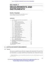
Measurement of damping and its relation to circuit resistance can be accomplished by a simple
procedure in the circuit of Fig. 3-1. Let R
a
be very large (say, 150 kΩ) and R
b
small (say, 1 Ω) so
that when E is a 1.5-V dry cell, the driving voltage in the local galvanometer loop is a few micro-
volts (say, 10 mV). Since circuital damping is related to total circuit resistance (R
c
ϩ R
b
ϩ R
g
), the
galvanometer resistance R
g
must be determined first. If R
c
is adjusted to a value that gives a con-
venient deflection and then to a new value R
c
′ for which the deflection is cut in half, we have R
g
ϭ
R
c
′ Ϫ 2R
c
Ϫ R
b

. Now, let R
c
be set at such a value that when the switch is closed, the overshoot is
readily observed. After noting the open-circuit deflection u
o
, the switch is closed and the peak
value u, of the first overswing, and the final deflection u
F
are noted. Then
g
1
being the relative damping corresponding to the circuit resistance R
1
ϭ R
g
ϩ R
b
ϩ R
c
. The switch
is now opened, and the first overswing u
2
past the open-circuit equilibrium position u
o
is noted. Then
g
o
being the open-circuit relative damping. The relative damping g
x
for any circuit resistance R

x
is
given by the relation
where it should be noted that the galvanometer resistance R
g
is included in both R
x
and R
1
. For crit-
ical damping R
d
can be computed by setting g
x
ϭ 1, and the external critical damping resistance
CDRX ϭ R
d
Ϫ R
g
.
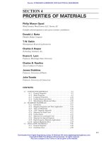
Galvanometer shunts are used to reduce the response of the galvanometer to a signal. However,
in any sensitivity-reduction network, it is important that relative damping be preserved for proper
operation. This can always be achieved by a suitable combination of series and parallel resistance.
In Fig. 3-2, let r be the external circuit resistance and R
g
the galvanometer resistance such that
r ϩ R
g
gives an acceptable damping (e.g., g ϭ 0.8) at maximum sensitivity. This damping will
be preserved when the sensitivity-reduction network (S, P) is inserted, if S ϭ (n Ϫ 1)r and P ϭ

nr/(n Ϫ 1), n being the factor by which response is to be reduced. The Ayrton-Mather shunt, shown
R
x
R
1
ϭ
g
1
Ϫ g
o
g
x
Ϫ g
o
ln
u
F
Ϫ u
o
u
2
Ϫ u
o
ϭ
p g
o
21 Ϫ g
2
o
ln

u
F
Ϫ u
o
u
1
Ϫ u
F
ϭ
p g
1
21 Ϫ g
2
1
FIGURE 3-1 Determination of relative damping.
FIGURE 3-2 Galvanometer shunt.
Beaty_Sec03.qxd 17/7/06 8:26 PM Page 3-7
Downloaded from Digital Engineering Library @ McGraw-Hill (www.digitalengineeringlibrary.com)
Copyright © 2006 The McGraw-Hill Companies. All rights reserved.
Any use is subject to the Terms of Use as given at the website.
MEASUREMENTS AND INSTRUMENTS*
3-8 SECTION THREE
in Fig. 3-3, may be used where the circuit resistance r is so high
that it exerts no appreciable damping on the galvanometer. R
ab
should be such that correct damping is achieved by R
ab
ϩ R
g
. In

this network, sensitivity reduction is
and the ratio of galvanometer current I
g
to line current I is
The ultimate resolution of a detection system is the magnitude of the signal it can discriminate
against the noise background present. In the absence of other noise sources, this limit is set by the
Johnson noise generated by electron thermal agitation in the resistance of the circuit. This is expressed
by the formula , where e is the rms noise voltage developed across the resistance R, k is
Boltzmann’s constant 1.4 ϫ 10
Ϫ23
J/K, u is the absolute temperature of the resistor in kelvin, and f
is the bandwidth over which the noise voltage is observed. At room temperature (300 K) and with the
assumption that the peak-to-peak voltage is 5 ϫ rms value, the peak-to-peak Johnson noise voltage
is 6.5 ϫ 10
Ϫ10
V. If, in a dc system, we use the approximation that f ϭ
1
/
3
t, where t is the
system’s response time, the Johnson voltage is 4 ϫ 10
Ϫ10
V (peak to peak).
By using reasonable approximations, it can be shown that the random brownian-motion
deflections of the moving system of a galvanometer, arising from impulses by the molecules in the air
around it, are equivalent to a voltage indication e ϭ 5 ϫ 10
Ϫ10
V (peak to peak), where R is cir-
cuit resistance and T is the galvanometer period in seconds. If the galvanometer damping is such that
its response time is t ϭ 2T/3 (for ), the Johnson noise voltage to which it responds is about

5 ϫ 10
Ϫ10
V (peak to peak). This value represents the limiting resolution of a galvanometer,
since its response to smaller signals would be obscured by the random excursions of its moving sys-
tem. Thus, a galvanometer with a 4-s-period would have a limiting resolution of about 2 nV in a 100-Ω
circuit and 1 nV in a 25-Ω circuit.
It is not surprising that one arrives at the same value from considerations either of random elec-
tron motions in the conductors of the measuring circuit or of molecular motions in the fluid that sur-
rounds the system. The resulting figure rests on the premise that the law of equipartition of energy
applies to the measuring system and that the galvanometer coil—a body with one degree of freedom—
is statically in thermal equilibrium with its surroundings.
Optical systems used with galvanometers and other indicating instruments avoid the necessity for a
mechanical pointer and thus permit smaller, simpler balancing arrangements because the mirror attached
to the moving system can be symmetrically disposed close to the axis of rotation. In portable instru-
ments, the entire system—source, lenses, mirror, scale—is generally integral with the instrument, and
the optical “pointer” may be folded one or more times by fixed mirrors so that it is actually much longer
than the mechanical dimensions of the instrument case. In some instances, the angular displacement may
be magnified by use of a cylindrical lens or mirror. For a wall- or bracket-mounted galvanometer, the
lamp and scale arrangement is external, and the length of the light-beam pointer can be controlled.
Whatever the arrangement, the pointer length cannot be indefinitely extended with consequent increase
in resolution at the scale. The optical resolution of such a system is, in any event, limited by image dif-
fraction, and this limit—for a system limited by a circular aperture—is , where a is the
angle subtended by resolvable points, l is the wavelength of the light, n is the index of refraction of the
image space, and d is the aperture diameter. In this case, d is the diameter of the moving-system mirror,
and n ϭ 1 for air. If we assume that points 0.1 mm apart can just be resolved by the eye at normal read-
ing distance, the resolution limit is reached at a scale distance of about 2 m in a system with a 1-cm mir-
ror, which uses no optical magnification. Thus, for the usual galvanometer, there is no profit in using a
mirror-scale separation greater than 2 m. Since resolution is a matter of subtended angle, the corre-
sponding scale distance is proportionately less for systems that make use of magnification.
The photoelectric galvanometer amplifier is a detector system in which the light beam from the

moving-system mirror is split between two photovoltaic cells connected in opposition, as shown
a < 1.2l/nd
2R/t
g < 0.8
2R/T
2R/t
2Rf
e ϭ !4kuRf
I
g
I
ϭ
R
ab
n(R
g
ϩ R
ab
)
n ϭ R
ac
/R
ab
FIGURE 3-3 Ayrton-Mather
universal shunt.
Beaty_Sec03.qxd 17/7/06 8:26 PM Page 3-8
Downloaded from Digital Engineering Library @ McGraw-Hill (www.digitalengineeringlibrary.com)
Copyright © 2006 The McGraw-Hill Companies. All rights reserved.
Any use is subject to the Terms of Use as given at the website.
MEASUREMENTS AND INSTRUMENTS*

MEASUREMENTS AND INSTRUMENTS 3-9
FIGURE 3-4 Photoelectric galvanometer amplifier.
in Fig. 3-4. As the mirror of the primary galvanometer turns in response to an input signal, the light
flux is increased on one of the photocells and decreased on the other, resulting in a current and thence
an enhanced signal in the circuit of the secondary (reading) galvanometer. Since the photocells
respond to the total light flux on their sensitive elements, the system is not subject to resolution lim-
itation by diffraction as is the human eye, and the ultimate resolution of the primary instrument—
limited only by its brownian motion and the Johnson noise of the input circuit—may be realized.
Electronic instruments for low-level dc signal detection are more convenient, more rugged, and
less susceptible to mechanical disturbances than is a galvanometer. However, considerable filtering,
shielding, and guarding must be used to minimize electrical interference and noise. On the other
hand, a galvanometer is an extremely efficient low-pass filter, and when operated to make optimal
use of its design characteristics, it is still the most sensitive low-level dc detector. Electronic detec-
tors generally make use of either a mechanical or a transistor chopper driven by an oscillator whose
frequency is chosen to avoid the local power frequency and its harmonics. This modulator converts
the dc input signal to ac, which is then amplified, demodulated, and displayed on an analog-type
indicating instrument or fed to a recording device or a signal processor.
AC detectors used for balancing bridge networks are usually tuned low-level amplifiers coupled
to an appropriate display device. The narrower the passband of the amplifier, the better the signal
resolution, since the narrow passband discriminates against noise of random frequency in the input
circuit. Adjustable-frequency amplifier-detectors basically incorporate a low-noise preamplifier fol-
lowed by a high-gain amplifier around which is a tunable feedback loop whose circuit has zero trans-
mission at the selected frequency so that the negative-feedback circuit controls the overall transfer
function and acts to suppress signals except at the selected frequency. The amplifier output may be
rectified and displayed on a dc indicating instrument, and added resolution is gained by introducing
phase selection at the demodulator, since the wanted signal is regular in phase, while interfering
noise is generally random. In detectors of this type, in phase and quadrature signals can be displayed
separately, permitting independent balancing of bridge components. Further improvement can result
from the use of a low-pass filter between the demodulator and the dc indicator such that the signal
of selected phase is integrated over an appreciable time interval up to a second or more.

3.1.3 Continuous EMF Measurements
A standard of emf may be either an electrochemical system or a Zener-diode-controlled circuit oper-
ated under precisely specified conditions. The Weston standard cell has a positive electrode of metal-
lic mercury and a negative electrode of cadmium-mercury amalgam (usually about 10% Cd). The
electrolyte is a saturated solution of cadmium sulfate with an excess of Cd
.
SO
4
.
8
/
3
H
2
O crystals,
usually acidified with sulfuric acid (0.04 to 0.08 N). A paste of mercurous sulfate and cadmium sul-
fate crystals over the mercury electrode is used as a depolarizer. The saturated cell has a substantial
temperature coefficient of emf. Vigoureux and Watts of the National Physical Laboratory have given
the following formula, applicable to cells with a 10% amalgam:
ϫ 10
Ϫ6
(t Ϫ 20)
3
Ϫ 0.000150 ϫ 10
Ϫ6
(t Ϫ 20)
4
E
t
ϭ E

20
Ϫ 39.39 ϫ 10
Ϫ6
(t Ϫ 20) Ϫ 0.903 ϫ 10
Ϫ6
(t Ϫ 20)
2
ϩ 0.00660
Beaty_Sec03.qxd 17/7/06 8:26 PM Page 3-9
Downloaded from Digital Engineering Library @ McGraw-Hill (www.digitalengineeringlibrary.com)
Copyright © 2006 The McGraw-Hill Companies. All rights reserved.
Any use is subject to the Terms of Use as given at the website.
MEASUREMENTS AND INSTRUMENTS*
3-10 SECTION THREE
where t is the temperature in degree Celsius. Since cells are frequently maintained at 28°C, the
following equivalent formula is useful:
These equations are general and are normally used only to correct cell emfs for small temperature
changes, that is, 0.05 K or less. For changes at that level, negligible errors are introduced by making
corrections. Standard cells should always be calibrated at their temperature of use (within 0.05 K) if
they are to be used at an accuracy of 5 ppm or better.
A group of saturated Weston cells, maintained at a constant temperature in an air bath or a stirred
oil bath, is quite generally used as a laboratory reference standard of emf. The bath temperature must
be constant within a few thousandths of a degree if the reference emf is to be reliable to a microvolt.
It is even more important that temperature gradients in the bath be avoided, since the individual limbs
of the cell have very large temperature coefficients (about +315 mV/°C for the positive limb and
−379 mV/°C for the negative limb—more than −50 mV/°C for the complete cell—at 28°C).
Frequently, two or three groups of cells are used, one as a reference standard which never leaves the
laboratory, the others as transport groups which are used for interlaboratory comparisons and for
assignment by a standards laboratory.
Precautions in Using Standard Cells

1. The cell should not be exposed to extreme temperatures—below 4°C or above 40°C.
2. Temperature gradients (differences between the cell limbs) should be avoided.
3. Abrupt temperature changes should be avoided—the recovery period after a sudden temperature
change may be quite extended; recovery is usually much quicker in an unsaturated than in a sat-
urated cell. Full recovery of saturated cells from a gross temperature change (e.g., from room
temperature to a 35°C maintenance temperature) can take up to 3 months. More significantly,
some cell emfs have been seen to exhibit a plateau in their response over a 2- to 3-week period
within a week or two after the temperature shock is sustained. This plateau can be as much as
5 ppm higher than the final stable value.
4. Current in excess of 100 nA should never be passed through the cell in either direction; actually,
one should limit current to 10 nA or less for as short a time as feasible in using the cell as a ref-
erence. Cells that have been short-circuited or subjected to excessive charging current drift until
chemical equilibrium in the cell is regained over an extended time period—as long as 9 months,
depending on the amount of charge involved.
Zener diodes or diode-based devices have replaced chemical cells as voltage references in com-
mercial instruments, such as digital voltmeters and voltage calibrators. Some of these instruments
have uncertainties below 10 ppm, instabilities below 5 ppm per month (including drift and random
uncertainties), and temperature coefficient of output as low as 2 ppm/°C.
The best devices, as identified in a testing in selection process, are available as solid-state volt-
age reference or transport standards. Such instruments generally have at least two outputs, one in the
range of 1.018 to 1.02 V for use as a standard cell replacement and the other in the range of 6.4 to
10 V, the output voltage of the reference device itself. The lower voltage is usually obtained via a
resistive divider.
Other features sometimes include a vernier adjustment for the lower voltage for adjusting to equal
the output of a given standard cell and internal batteries for complete isolation. Such devices have
performance approaching that of standard cells and can be used in many of the same applications.
Some have stabilities (drift rate and random fluctuations) as low as 2 to 3 ppm per year and temper-
ature coefficient of 0.1 ppm/°C.
The current through the reverse-biased junction of a silicon diode remains very small until the
bias voltage exceeds a characteristic V

z
in magnitude, at which point its resistance becomes abruptly
ϫ 10
Ϫ6
(t Ϫ 28)
3
Ϫ 0.0001497 ϫ 10
Ϫ6
(t Ϫ 28)
4
E
t
ϭ E
28
Ϫ 52.899 ϫ 10
Ϫ6
(t Ϫ 28) Ϫ 0.80265 ϫ 10
Ϫ6
(t Ϫ 28)
2
ϩ 0.001813
Beaty_Sec03.qxd 17/7/06 8:26 PM Page 3-10
Downloaded from Digital Engineering Library @ McGraw-Hill (www.digitalengineeringlibrary.com)
Copyright © 2006 The McGraw-Hill Companies. All rights reserved.
Any use is subject to the Terms of Use as given at the website.
MEASUREMENTS AND INSTRUMENTS*
MEASUREMENTS AND INSTRUMENTS 3-11
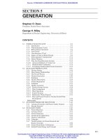
FIGURE 3-5 General purpose constant-current potentiometer.
very low so that the voltage across the junction is little affected by the junction current. Since the
voltage-current relationship is repeatable, the diode may be used as a standard of voltage as long as

its rated power is not exceeded.
However, since V
z
is a function of temperature, single junctions are rarely used as voltage refer-
ences in precise applications. Since a change in temperature shifts the I-V curve of a junction, the
use of a forward-biased junction in series with Zener diode permits a current level to be found at
which changes in Zener voltage from temperature changes are compensated by changes in the volt-
age drop across the forward-biased junction.
Devices using this principle fall into two categories: the temperature-compensated Zener diode,
in which two diodes are in series opposition, and the reference amplifier, in which the Zener diode
is in series with the base-emitter junction of an appropriate npn silicon transistor. In each case, the
two elements may be on the same substrate for temperature uniformity. In some precision devices,
the reference element is in a temperature-controlled oven to permit even greater immunity to tem-
perature fluctuations.
Potentiometers are used for the precise measurement of emf in the range below 1.5 V. This is
accomplished by opposing to the unknown emf an equal IR drop. There are two possibilities: either
the current is held constant while the resistance across which the IR drop is opposed to the unknown
is varied, or current is varied in a fixed resistance to achieve the desired IR drop.
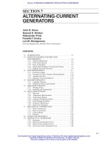
Figure 3-5 shows schematically most of the essential features of a general-purpose constant-
current instrument. With the standard-cell dial set to read the emf of the reference standard cell, the
potentiometer current I is adjusted until the IR drop across 10 of the coarse-dial steps plus the drop
to the set point on the standard-cell dial balances the emf of the reference cell. The correct value of
current is indicated by a null reading of the galvanometer in position G
1
. This adjustment permits the
potentiometer to be read directly in volts. With the galvanometer in position G
2
, the unknown emf is
balanced by varying the opposing IR drop. Resistances used from the coarse and intermediate dials
and the slide wire are adjusted until the galvanometer again reads null, and the unknown emf can be

read directly from the dial settings. The ratio of the unknown and reference emfs is precisely the ratio
as the resistances for the two null adjustments, provided that the current is the same.
Beaty_Sec03.qxd 17/7/06 8:26 PM Page 3-11
Downloaded from Digital Engineering Library @ McGraw-Hill (www.digitalengineeringlibrary.com)
Copyright © 2006 The McGraw-Hill Companies. All rights reserved.
Any use is subject to the Terms of Use as given at the website.
MEASUREMENTS AND INSTRUMENTS*
3-12 SECTION THREE
FIGURE 3-6 Constant-resistance potentiometer.
The switching arrangement is usually such that the galvanometer can be shifted quickly between
the G
2
and G
1
positions to check that the current has not drifted from the value at which it was stan-
dardized. It will be noted that the contacts of the coarse-dial switch and slide wire are in the gal-
vanometer branch of the circuit. At balance, they carry no current, and their contact resistance does
not contribute to the measurement. However, there can be only two noncontributing contact resis-
tances in the network shown; the switch contacts for adjusting the intermediate-dial position do carry
current, and their resistance does enter the measurement. Care is taken in construction that the resis-
tances of such current-carrying contacts are low and repeatable, and frequently, as in the example
illustrated, the circuit is arranged so that these contributing contacts carry only a fraction of the ref-
erence current, and the contribution of their IR drop to the measurement is correspondingly reduced.
Another feature of many general-purpose potentiometers, illustrated in the diagram, is the
availability of a reduced range. The resistances of the range shunts have such values that at the
0.1 position of the range-selection switch, only a tenth of the reference current goes through
the measuring branch of the circuit, and the range of the potentiometer is correspondingly
reduced. Frequently, a ϫ 0.01 range is also available.
In addition to the effect of IR drops at contacts in the measuring circuit, accuracy limits are also
imposed by thermal emfs generated at circuit junctions. These limiting factors are increasingly

important as potentiometer range is reduced. Thus, in low-range or microvolt potentiometers, spe-
cial care is taken to keep circuit junctions and contact resistances out of the direct measuring circuit
as much as possible, to use thermal shielding, and to arrange the circuit and galvanometer keys so
that temperature differences will be minimized between junction points that are directly in the mea-
suring circuit. Generally also, in microvolt potentiometers, the galvanometer is connected to the cir-
cuit through a special thermofree reversing key so that thermal emfs in the galvanometer can be
eliminated from the measurement—the balance point being that which produces zero change in gal-
vanometer deflections on reversal.
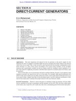
An example of the constant-resistance potentiometer is shown in the simplified diagram in Fig. 3-6.
It consists basically of a constant-current source, a resistive divider D (used in the current-divider mode),
and a fixed resistor R in which the current (and the IR drop) are determined by the setting of the divider.
The output of the current source is adjusted by equating the emf of a standard cell to an equal IR drop
as shown by the dashed line. This design lends itself to multirange operation by using tap points on the
resistor R. Its accuracy depends on the uniformity of the divider, the location of the tap points on R, and
the stability of the current source.
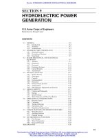
Another type of constant-resistance potentiometer, operating from a current comparator which
senses and corrects for inequality of ampere-turns in two windings threading a magnetic core, is
shown in Fig. 3-7. Two matched toroidal cores wound with an identical number of turns are excited
by a fixed-frequency oscillator. The fluxes induced in the cores are equal and oppositely directed, so
they cancel with respect to a winding that encloses both. In the absence of additional magnetomo-
tive force (mmf), the detector winding enclosing both cores receives no signal.
If, in another winding A enclosing both cores, we inject a direct current, its mmf reinforces the
flux in one core and opposes the other. The net flux in the detector winding induces a voltage in it.
This signal is used to control current in another winding B which also threads both cores. When the
mmf of B is equal to and opposite that of A, the detector signal is zero and the ampere-turns of A and
B are equal. Thus, a constant current in an adjustable number of turns is matched to a variable cur-
rent in a fixed number of turns, and the voltage drop I
B
R is used to oppose the emf to be measured.
Beaty_Sec03.qxd 17/7/06 8:26 PM Page 3-12

Downloaded from Digital Engineering Library @ McGraw-Hill (www.digitalengineeringlibrary.com)
Copyright © 2006 The McGraw-Hill Companies. All rights reserved.
Any use is subject to the Terms of Use as given at the website.
MEASUREMENTS AND INSTRUMENTS*
MEASUREMENTS AND INSTRUMENTS 3-13
FIGURE 3-7 Current-comparator potentiometer.
The system is made direct-reading in voltage units (in terms of the turns ratio B/A) by adjusting the
constant-current source with the aid of a standard-cell circuit (not shown in the figure). This type of
potentiometer has an advantage over those whose continuing accuracy depends on the stability of a resis-
tance ratio; the ratio here is the turns ratio of windings on a common core, dependent solely on conduc-
tor position and hence not subject to drift with time.
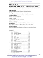
Decade voltage dividers generally use the Kelvin-
Varley circuit arrangement shown in Fig. 3-8. It will
be seen that two elements of the first decade are
shunted by the entire second decade, whose total resis-
tance equals the combined resistance of the shunted
steps of decade I. The two sliders of decade I are
mechanically coupled and move together, keeping the
shunted resistance constant regardless of switch posi-
tion. Thus, the current divides equally between decade
II and the shunted elements of decade I, and the volt-
age drop in decade II equals the drop in one unshunted
step of decade I. The effect of contact resistance at the
switch points is somewhat diminished because of the
division of current. The Kelvin-Varley principle is
used in succeeding decades except the final one,
which has only a single switch contact. Such voltage dividers may have as many as eight decades
and have ratio accuracies approaching 1 part in 10
6
of input.

Spark gaps provide a means of measuring high voltages. The maximum gap which a given volt-
age will break down depends on air density, gap geometry, crest value of the voltage, and other fac-
tors (see Sec. 27). Sphere gaps constitute a recognized means for measuring crest values of
alternating voltages and of impulse voltages. IEEE Standard 4 has tables of sparkover voltages for
spheres ranging from 6.25 to 200 cm in diameter and for voltages from 17 to 2500 kV. Sphere gap
voltage tables are also available in ANSI Standard 68.1 and in IEC Publication 52.
3.1.4 Continuous Current Measurements
Absolute current measurement relates the value of the current unit—the ampere—to the prototype
mechanical units of length, mass, and time—the meter, the kilogram, and the second—through force
measurements in an instrument called a current balance. Such instruments are to be found generally
only in national standards laboratories, which have the responsibility of establishing and maintain-
ing the electrical units. In a current balance, the force between fixed and movable coils is opposed
by the gravitational force on a known mass, the balance equation being I
2
(0M/0X) ϭ mg. The con-
struction of the coil system is such that the rate of change with displacement of mutual inductance
between fixed and moving coils can be computed from measured coil dimensions. Absolute current
determinations are used to assign the emf of reference standard cells. A 1-Ω resistance standard is
connected in series with the fixed- and moving-coil system, and its drop is compared with the emf
of a cell during the force measurement. Thus, the National Reference Standard of voltage is derived
from absolute ampere and ohm determinations.
FIGURE 3-8 Decade voltage divider.
Beaty_Sec03.qxd 17/7/06 8:26 PM Page 3-13
Downloaded from Digital Engineering Library @ McGraw-Hill (www.digitalengineeringlibrary.com)
Copyright © 2006 The McGraw-Hill Companies. All rights reserved.
Any use is subject to the Terms of Use as given at the website.
MEASUREMENTS AND INSTRUMENTS*
3-14 SECTION THREE
The potentiometer method of measuring continuous currents is commonly used where a value
must be more accurate than can be obtained from the reading of an indicating instrument. The cur-

rent to be measured is passed through a four-terminal resistor (shunt) of known value, and the volt-
age developed between its potential terminals is measured with a potentiometer. If the current is
small so that there is no significant temperature rise in the shunt, the measurement accuracy can be
0.01% or better. In general, the accuracy of potentiometer measurements of continuous currents is
limited by how well the shunt resistance is known under operating conditions.
Measurement of very small continuous currents, down to 10
–17
A, have been accomplished by
means of electrometer tubes—vacuum tubes designed so that the grid has practically no leakage cur-
rent either over its insulating supports or to the cathode. The current to be measured flows through
a very high resistance (up to 10
12
Ω), and the voltage drop is impressed on the grid of an electrom-
eter tube. The plate current is observed and the voltage drop is duplicated by producing the plate cur-
rent with a known adjustable voltage. The current can then be calculated from the voltage and
resistance.
3.1.5 Analog Instruments
Analog instruments are electromechanical devices in which an electrical quantity is measured by
conversion to a mechanical motion. Such instruments can be classified according to the principle on
which the instrument operates. The usual types are permanent-magnet moving-coil, moving-iron,
dynamometer, and electrostatic. Another grouping is on the basis of use: panel, switchboard,
portable, and laboratory-standard. Accuracy also can be the basis of classification. Details concern-
ing performance and other specifications are to be found in ANSI Standard C39.1, Requirements for
Electrical Analog Indicating Instruments.
Permanent-magnet moving-coil instruments are the most common type in general use. The oper-
ating mechanism consists of a coil of fine wire suspended in such a manner that it can rotate in an
annular gap which has a radial magnetic field. The torque, generated by the current in the moving
coil reacting to the magnetic field of the gap, is opposed by some form of spring restraint. The
restraint may be a helical spring, in which case the coil is supported by a pivot and jewel, or both the
support and the angular restraint is by means of a taut-band suspension.

The position which the coil assumes when the torque and spring restraint are balanced is indi-
cated by either a pointer or a light beam on a scale. The scale is calibrated in units suitable to the
application: volts, milliamperes, etc. To the extent that the magnetic field is uniform, the spring
restraint linear, and the coil positioning symmetrical, the deflection will be linearly proportional to
the ampere-turns in the coil.
Because the field of the permanent magnet is unidirectional, reversal of the coil current will
reverse the torque so that the instrument will deflect only with direct current in the moving coil.
Scales are usually provided with the zero-current position at the left to allow a full-range deflection.
However, where measurement is required with either polarity, a zero center scale position is used.
The coil is limited in its ability to carry current to 50 or 100 mA.
Rectifiers and thermoelements are used with permanent-magnet moving-coil instruments to pro-
vide ac operation. The addition of a rectifier circuit, usually in the form of a bridge, gives an instru-
ment in which the deflection is in terms of the average value of the voltage or current. It is customary
to label the scale in terms of 1.11 times the average; this is the correct waveform factor to read the
rms value of a sine wave. If the rectifier instrument is used to measure severely nonsinusoidal wave-
forms, large errors will result. The high sensitivity that can be obtained with the rectifier type of
instrument and its reasonable cost make it widely used.
To provide a true rms reading with the permanent-magnet moving-coil instrument, a thermoelement
is the usual converter. The current to be measured is fed through a resistance of such value that it will
heat appreciably. A thermocouple is placed in intimate thermal contact with the heater resistance, and
the output of the couple is used to energize a permanent-magnet moving-coil instrument. The instrument
deflection of such a combination is proportional to the square of the current; using a square-root factor
in drawing the scale allows it to be read in terms of the rms value of the current. For high-sensitivity use,
the thermoelement is placed in an evacuated bulb to eliminate convection heat loss.
Beaty_Sec03.qxd 17/7/06 8:26 PM Page 3-14
Downloaded from Digital Engineering Library @ McGraw-Hill (www.digitalengineeringlibrary.com)
Copyright © 2006 The McGraw-Hill Companies. All rights reserved.
Any use is subject to the Terms of Use as given at the website.
MEASUREMENTS AND INSTRUMENTS*
MEASUREMENTS AND INSTRUMENTS 3-15

The prime advantage of the thermoelement instrument is the high frequency at which it will operate
and the rms indication. The upper frequency limit is determined by the skin effect in the heater.
Instruments have been built with response to several hundred megahertz. There is one very important
limitation to these instruments. The heater must operate at a temperature of 100°C or more to provide
adequate current to the movement. Overrange of the current will cause heater temperature to increase as
the square of the current. It is possible to burn out the heater with relatively small overloads.
Moving-iron instruments are widely used at power frequencies. The radial-vane moving-iron type
operates by current in the coil which surrounds two magnetic vanes, one fixed and one that can rotate
in such a manner as to increase the spacing between them. Current in the coil causes the vanes to be
similarly magnetized and so to repel each other. The torque produced by the moving vane is pro-
portional to the square of the current and is independent of its polarity.
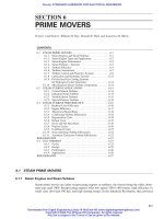
Figure 3-9 shows two ways in which a wattmeter
may be connected to measure power in a load. With the
moving coil connected at A, the instrument will read
high by the amount of power used by the moving-coil
circuit. If connection is made at B, the wattmeter will
read high by the power dissipated in the field coils.
When using sensitive, low-range meters, it is necessary
to correct for this error. Commercial instruments are
available for ranges from a fraction of a watt to several
hundred watts self-contained. Range extensions are
obtained with current and voltage transformers. In
specifying wattmeters, it is necessary to state the cur-
rent and voltage ranges as well as the watt range.
Electrostatic voltmeters are actually voltage-operated
in contrast to all the other types of analog instruments, which are current-operated. In an electrosta-
tic voltmeter, fixed and movable vanes are so arranged that a voltage between them causes attraction
to rotate the movable vane. The torque is proportional to the energy stored in the capacitance, and
thus to the voltage squared, permitting rms indication.
Electrostatic instruments are used for voltage measurements where the current drain of other

types of instrument cannot be tolerated. Input resistance (due to insulation leakage) amounts to 10
13
Ω
approximately for a range of 100 V (the lowest commercially available) to 3 ϫ 10
15
Ω for 100,000-V
instruments (the highest commonly available). Capacitance ranges from about 300 pF for the lower
ranges to 10 pF for the highest. Multirange instruments in the lower ranges (100 to 5000 V) are fre-
quently made with capacitive dividers which make them inoperable on direct voltage, since the series
capacitor blocks out dc. Other multirange instruments use a mechanical movement of the fixed elec-
trode to change ranges. These can be used on dc or ac, as can all single-range voltmeters.
Electronic voltmeters vary widely in performance characteristics and frequency range cov-
ered, depending on the circuitry used. A common type uses an initial diode to charge a capaci-
tor. This may be followed by a stabilized amplifier with a microammeter as indicator. Range
may be selected by appropriate cathode resistors in the amplifier section. Such instruments nor-
mally have very high input impedance (a few picofarads), respond to peak voltage, and are suit-
able for use to very high frequencies (100 MHz or more). While the response is to peak voltage,
the scale of the indicating element may be marked in terms of rms for a sine-wave input, that is,
0.707 ϫ peak voltage. Thus, for a nonsinusoidal input, the scale (read as rms volts) may include
a serious waveform error, but if the scale reading is multiplied by 1.41, the result is the value of
the peak voltage.
An alternative network, used in some electronic voltmeters, is an attenuator for range selection,
followed by an amplifier and finally a rectifier and microammeter. This system has substantially lower
input impedance, and limits of frequency range are fixed by the characteristics of the amplifier. The
response in this arrangement may be to average value of the input signal, but again, the scale mark-
ing may be in terms of rms value for a sine wave. In this case also, the waveform error for nonsinu-
soidal input must be borne in mind, but if the scale reading is divided by 1.11, the average value is
obtained. Within these limitations, accuracy may be as good as 1% of full-scale indication in some-
types of electronic voltmeter, although in many cases a 2 to 5% accuracy may be anticipated.
FIGURE 3-9 Alternative wattmeter connections.

Beaty_Sec03.qxd 17/7/06 8:26 PM Page 3-15
Downloaded from Digital Engineering Library @ McGraw-Hill (www.digitalengineeringlibrary.com)
Copyright © 2006 The McGraw-Hill Companies. All rights reserved.
Any use is subject to the Terms of Use as given at the website.
MEASUREMENTS AND INSTRUMENTS*
3-16 SECTION THREE
3.1.6 DC to AC Transfer
General transfer capability is essential to the measurement of voltage, current, power, and energy.
The standard cell, the unit of voltage which it preserves, and the unit of current derived from it in
combination with a standard of resistance are applicable only to the measurement of dc quantities,
while the problems of measurement in the power and communications fields involve alternating volt-
ages and currents. It is only by means of transfer devices that one can assign the values of ac quan-
tities or calibrate ac instruments in terms of the basic dc reference standards. In most instances, the
rms value of a voltage or current is required, since the transformation of electrical energy to other forms
involves the square of voltages or currents, and the transfer from direct to alternating quantities is made
with devices that respond to the square of current or voltage. Three general types of transfer instruments
are capable of high-accuracy rms measurements: (1) electrodynamic instruments—which depend on
the force between current-carrying conductors; (2) electrothermic instruments—which depend on the
heating effect of current; and (3) electrostatic instruments—which depend on the force between elec-
trodes at different potentials. While two of these depend on current and the third on voltage, the use of
series and shunt resistors makes all three types available for current or voltage transfer. Traditional
American practice has been to use electrodynamic instruments for current and voltage transfer as well
as power transfer from direct to alternating current, but recent developments in thermoelements have
improved their transfer characteristics until they are now the preferred means for current and voltage
transfer, although the electrodynamic wattmeter is still the instrument of choice for power transfer up
to 1 kHz.
Electrothermic transfer standards for current and voltage use a thermoelement consisting of a
heater and a thermocouple. In its usual form, the heater is a short, straight wire suspended by two
supporting lead-in wires in an evacuated glass bulb. One junction of a thermocouple is fastened to
its midpoint and is electrically insulated from it with a small bead. The thermal emf—5 to 10 mV at

rated current in a conventional element—is a measure of heater current. Multijunction thermo-
elements having a number of couples in series along the heater also have been used in transfer mea-
surements. Typical output is 100 mV for an input power of 30 mW.
3.1.7 Digital Instruments
Digital voltmeters (DVMs), displaying the measured voltage as a set of numerals, are analog-to-digital
converters in which an unknown dc voltage is compared with a stable reference voltage. Internal
fixed dividers or amplifiers extend the voltage ranges. For ac measurements, dc DVMs are preceded
by ac-to-dc converters. DVMs are widely used as laboratory, portable, and panel instruments because
of their convenience, accuracy, and speed. Automatic range changing and polarity indication, free-
dom from reading errors, and the availability of outputs for data acquisition or control are added
advantages. Integrated circuits and modern techniques have greatly increased their reliability and
reduced their cost. Full-scale accuracies range from about 0.5% for three-digit panel instruments to
1 ppm for eight-digit laboratory dc voltmeters and 0.016% for ac voltmeters.
Successive-approximation DVMs are automatically operated dc potentiometers. These may be
based on resistive voltage or current divider techniques or on dc current comparators. A comparator
in a series of steps adjusts a discrete fraction of the reference voltage (by current or voltage division
in a resistance network) until it equals the unknown. Various “logic schemes” have been used to
accomplish this, and the stepping relays of earlier models have been replaced by electronic or reed
switches. Filters reduce input noise (which could prevent a final display) but generally increase the
response time. Accuracy depends chiefly on the reference voltage and the ratios of the resistance
network.
Voltage-to-frequency-converter (V/f) DVMs generate a ramp voltage at a rate proportional to the
input until it equals a fixed voltage, returns the ramp to the starting point, and repeats. The number
of pulses (ramps) generated in a fixed time is proportional to the input and is counted and displayed.
Since it integrates over the counting time, a V/f DVM has excellent input-noise rejection. The ramp is
usually generated by an operational integrator (a high-gain operational amplifier with a capacitor in
the feedback loop so that its output is proportional to the integral of the input voltage). The capacitor
Beaty_Sec03.qxd 17/7/06 8:26 PM Page 3-16
Downloaded from Digital Engineering Library @ McGraw-Hill (www.digitalengineeringlibrary.com)
Copyright © 2006 The McGraw-Hill Companies. All rights reserved.

Any use is subject to the Terms of Use as given at the website.
MEASUREMENTS AND INSTRUMENTS*
MEASUREMENTS AND INSTRUMENTS 3-17
is discharged each time by a pulse of constant and opposite charge, and the time interval of the
counter is chosen so that the number of pulses makes the DVM direct-reading. Accuracy depends on
the integrator and on the charge of the pulse generator, which contains the reference voltage.
Dual-slope DVMs generate a voltage ramp at a rate proportional to the input voltage V
i
for a fixed
time t
1
. The ramp input is then switched to a reference voltage V
r
of the opposite polarity for a time
t
2
until the starting level is reached. Pulses with a fixed frequency f are accumulated in a counter,
with N
1
counts during t
1
. The counter resets to zero and accumulates N
2
counts during t
2
. Thus, t
1
ϭ
N
1

f and t
2
ϭ N
2
f.
If the slope of the linear ramp is m ϭ kV, the ramp voltage is V
o
ϭ mt ϭ kVt. Thus V
i
t
1
ϭ V
r
t
2
, so
V
i
ϭ V
r
N
2
/N
1
. The time t
1
is controlled by the counter to make N
2
direct-reading in appropriate units. In
principle, the accuracy is not dependent on the constants of the ramp generator or the frequency of the

pulses. A single operational integrator, switched to either input or reference voltage, generates the ramps.
Since there are few critical components, integrated circuits are feasible, leading to simplicity and relia-
bility as well as high accuracy. Because this is an integrating DVM, noise rejection is excellent.
In pulse-width conversion meters, an integrating circuit and matched comparators are used to pro-
duce trains of positive and negative pulses whose relative widths are a linear function of any dc input.
The difference in positive and negative pulse widths can be measured using counting techniques, and
very high resolution and accuracy (up to 1 ppm, relative to an internal voltage reference) can be
achieved by integrating the counting over a suitable time period.
Average ac-to-dc converters contain an operational rectifier (an operational amplifier with a rec-
tifier in the feedback circuit), followed by a filter, to obtain the rectified average value of the ac volt-
age. The operational amplifier greatly reduces errors of nonlinearity and forward voltage drop of the
rectifier. For convenience, the output voltage is scaled so that the dc DVM connected to it indicates
the rms value of a sine wave. Large errors can result for other waveforms, up to h/n%, with h% of
the nth harmonic in the wave, if n is an odd number. For example, with 3% of third harmonic, the
error can be as much as 1%, depending on the phase of the harmonic.
Electronic multipliers and other forms of rms-responding ac-to-dc converters eliminate this wave-
form error but are generally more complex and expensive. In one version, the feedback rms circuit
shown in Fig. 3-10, the two inputs of the multiplier M
1
are connected together so that the instantaneous output
of M is v
i
2
/V
o
. The operational filter F(RC circuit and
operational amplifier) makes V
o
ϭ V
2

i
/V
o
, where V
2
i
is
the square of the rms value. Thus, V
o
ϭ V
i
. The con-
version accuracy approaches 0.1% up to 20 kHz in
transconductance or logarithmic multipliers, without
requiring a wide dynamic range in the instrument,
because of the internal feedback. A series of diodes, biased to conduct at different voltage levels, can
provide an excellent approximation to a square-law function in a feedback circuit like that of Fig. 3-10.
Specifications for DVMs should follow the recommendations of ANSI Standard C39.7,
Requirements for Digital Voltmeters. Accuracy should be stated as the overall limit of error for a
specified range of operating conditions. It should be in percent of reading plus percent of full scale
and may be different for different frequency and voltage ranges. Accuracy at a narrow range of ref-
erence conditions is also often specified for laboratory use. The input configuration (two-terminal,
three-terminal unguarded, three- or four-terminal guarded) is important. Number of digits and “over-
range” also should be stated.
Errors and Precautions. Because of the sensitivity of DVMs, a number of precautions should be
taken to avoid in-circuit errors from ground loops, input noise, etc. The high input impedance of
most types makes input loading errors negligible, but this should always be checked. On dc millivolt
ranges, unwanted thermal emfs should be checked as well as the normal-mode rejection of ac line-
frequency voltage across the input terminals. Two-terminal DVMs (chassis connected to one input
as well as to line ground) may measure unwanted voltages from ground currents in the common line.

Errors are greatly reduced in three-terminal DVMs (chassis connected to line ground only) and
are generally negligible with guarded four-terminal DVMs (separate guard chassis surrounding the
FIGURE 3-10 Electronic rms ac-to-dc converter.
Beaty_Sec03.qxd 17/7/06 8:26 PM Page 3-17
Downloaded from Digital Engineering Library @ McGraw-Hill (www.digitalengineeringlibrary.com)
Copyright © 2006 The McGraw-Hill Companies. All rights reserved.
Any use is subject to the Terms of Use as given at the website.
MEASUREMENTS AND INSTRUMENTS*
3-18 SECTION THREE
measuring circuit). Such DVMs have very high common-mode rejection. Some types of DVMs
introduce small voltage spikes or currents to the measuring circuit, often from internal switching
transients, which may cause errors in low-level circuits.
Digital multimeters are DVMs with added circuitry to measure quantities such as dc voltage ratio,
dc and ac current, and resistance. Voltage ratio is measured by replacing the reference voltage with one
of the unknowns. For current, the voltage across an internal resistor carrying the current is measured
by the DVM. For resistance, a fixed reference current is generated and applied to the unknown resis-
tor. The voltage across the resistor is measured by the DVM. Several ranges are provided in each case.
3.1.8 Instrument Transformers
The material that follows is a brief summary of information on instrument transformers as measure-
ment elements. For more extensive information, consult American National Standard C57.13,
Requirement for Instrument Transformers; American National Standards Institute; American
National Standard C12, Code for Electricity Metering; Electrical Meterman’s Handbook, Edison
Electric Institute; manufacturer’s literature; and textbooks on electrical measurements.
AC range extension beyond the reasonable capability of indicating instruments is accomplished
with instrument transformers, since the use of heavy-current shunts and high-voltage multipliers
would be prohibitive both in cost and power consumption. Instrument transformers are also used to
isolate instruments from power lines and to permit instrument circuits to be grounded.
The current circuits of instruments and meters normally have very low impedance, and current
transformers must be designed for operation into such a low-impedance secondary burden. The insu-
lation from the primary to secondary of the transformer must be adequate to withstand line-to-

ground voltage, since the connected instruments are usually at ground potential. Normal design is
for operation with a rated secondary current of 5 A, and the input current may range upward to many
thousand amperes. The potential circuits of instruments are of high impedance, and voltage trans-
formers are designed for operation into a high-impedance secondary burden. In the usual design, the
rated secondary voltage is 120 V, and instrument transformers have been built for rated primary volt-
ages up to 765 kV.
With the development of higher transmission-line voltages (350 to 765 kV) and intersystem ties at
these levels, the coupling-capacitor voltage
transformer (CCVT) has come into use for
metering purposes to replace the conventional
voltage transformer, which, at these voltages, is
bulkier and more costly. The metering CCVT,
shown in Fig. 3-11, consists of a modular
capacitive divider which reduces the line
voltage V
1
to a voltage V
2
(10–20 kV), with a
series-resonant inductor to tune out the high
impedance and make available energy transfer
across the divider to operate the voltage trans-
former which further reduces the voltage to V
M
,
the metering level. Required metering accuracy
may be 0.3% or better.
Instrument transformers are broadly classified in two general types: (1) dry type, having
molded insulation (sometimes only varnish-impregnated paper or cloth) usually intended for
indoor installation, although large numbers of modern transformers have molded insulation suit-

able for outdoor operation on circuits up to 15 kV to ground; and (2) liquid-filled types in steel
tanks with high-voltage primary terminals, intended for installation on circuits above 15 kV. They
are further classified according to accuracy: (1) metering transformers having highest accuracy,
usually at relatively low burdens; and (2) relaying and control transformers which in general have
higher burden capacity and lower accuracy, particularly at heavy overloads. This accuracy classi-
fication is not rigid, since many transformers, often in larger sizes and higher voltage ratings, are
suitable for both metering and control purposes.
FIGURE 3-11 CCTV metering arrangement.
Beaty_Sec03.qxd 17/7/06 8:26 PM Page 3-18
Downloaded from Digital Engineering Library @ McGraw-Hill (www.digitalengineeringlibrary.com)
Copyright © 2006 The McGraw-Hill Companies. All rights reserved.
Any use is subject to the Terms of Use as given at the website.
MEASUREMENTS AND INSTRUMENTS*
MEASUREMENTS AND INSTRUMENTS 3-19
Another classification differentiates between single and multiple ratios. Multiple primary wind-
ings, sometimes arranged for series-parallel connection, tapped primary windings, or tapped sec-
ondary windings, are employed to provide multiple ratios in a single piece of equipment. Current
transformers are further classified according to their mechanical structure: (1) wound primary, hav-
ing more than one turn through the core window; (2) through type, wherein the circuit conductor
(cable or busbar) is passed through the window; (3) bar type, having a bar, rod, or tube mounted in
the window; and (4) bushing type, that is, through type intended for mounting on the insulating bush-
ing of a power transformer or circuit breaker.
Current transformers, whose primary winding is series connected in the line, serve the double
purposes of (1) convenient measurement of large currents and (2) insulation of instruments, meters,
and relays from high-voltage circuits. Such a transformer has a high-permeability core of relatively
small cross section operated normally at a very low flux density. The secondary winding is usually
in excess of 100 turns (except for certain small low-burden through-type current transformers used
for metering, where the secondary turns may be as low as 40), and the primary is of few turns and
may even be a single turn or a section of a bus bar threading the core. The nominal current ratio of
such a transformer is the inverse of the turns ratio, but for accurate current measurement, the actual

ratio must be determined under loading corresponding to use conditions. For accurate power and
energy measurement, the phase angle between the secondary and reversed primary phasor also must
be known for the use condition. Insulation of primary from secondary and core must be sufficient to
withstand, with a reasonable safety factor, the voltage to ground of the circuit into which it is con-
nected; secondary insulation is much less, since the connected instrument burden is at ground poten-
tial or nearly so.
The overload capacity of station-type current transformers and the mechanical strength of the
winding and core structure must be high to withstand possible short circuits on the line. Various com-
pensation schemes are used in many transformers to retain ratio accuracy up to several times rated
current. The secondary circuit—the current elements of connected instruments or relays—must
never be opened while the transformer is excited by primary current, because high voltages are
induced which may be hazardous to insulation and to personnel and because the accuracy of the
transformer may be adversely affected.
Voltage transformers (potential transformers) are connected between the lines whose potential
difference is to be determined and are used to step the voltage down (usually to 120 V) and to sup-
ply the voltage circuits of the connected instrument burden. Their basic construction is similar to that
of a power transformer operating at the same input voltage, except that they are designed for opti-
mal performance with the high-impedance secondary loads of the connected instruments. The core
is operated at high flux density, and the insulation must be appropriate to the line-to-ground voltage.
Standard burdens and standard accuracy requirements for instrument transformers are given in
American National Standard C57.13 (see Sec. 28).
Accuracy. Most well-designed instrument transformers (provided they have not been damaged or
incorrectly used) have sufficient accuracy for metering purposes. See Sec. 10 for typical accuracy curves.
Where higher accuracy is required, see Appendix D of ANSI C12, The Code for Electricity Metering.
Another comparison method uses a “standard” transformer of the same nominal rating as the one
being tested. Accuracies of 0.01% are attainable. Commercial test sets are available for this work and are
widely used in laboratory and field tests. Commercial test sets based on the current-comparator method
and capable of 0.001% accuracy are also available. For further details, see ANSI Standard C57.13.
3.1.9 Power Measurement
Electronic wattmeters of 0.1% or better accuracy may be based on a pulse-area principle. Voltages

proportional to the applied voltage and to the current (derived from resistors or transformers) gov-
ern the height and width of a rectangular pulse so that the area is proportional to the instantaneous
power. This is repeated many times during a cycle, and its average represents active power. Average
power also can be measured by a system which samples instantaneous voltage and current repeat-
edly, at predetermined intervals within a cycle. The sampled signals are digitized, and the result is
Beaty_Sec03.qxd 17/7/06 8:26 PM Page 3-19
Downloaded from Digital Engineering Library @ McGraw-Hill (www.digitalengineeringlibrary.com)
Copyright © 2006 The McGraw-Hill Companies. All rights reserved.
Any use is subject to the Terms of Use as given at the website.
MEASUREMENTS AND INSTRUMENTS*
3-20 SECTION THREE
computed by numerical integration. The response of such a system has been found to agree with that
of a standard electrodynamic wattmeter within 0.02% from dc to 1 kHz. Depending on sampling
speed, measurements can be made to higher frequencies with somewhat reduced accuracy. In the
digital instrument, the multiplication involves discrete numbers and thus has no experimental error
except for rounding. Such an arrangement is well-adapted to the measurement of power in situations
where current or voltage waveforms are badly distorted.
In the thermal wattmeter, where the arrangement is such that if one current v is proportional to
instantaneous load voltage and another i is proportional to load current, their sum is applied to one
thermal converter and their difference to another. Assuming identical quadratic response of the con-
verters, their differential output may be represented as
which is by definition average power. Multijunction thermal converters with outputs connected differ-
entially are used for the ac-dc transfer of power, with ac and dc current and voltage signals applied
simultaneously to both heaters. DC feedback to current input speeds response and maintains thermal
balance between heaters, and the output meter becomes a null indicator. This mode of operation can
eliminate the requirement for exact quadrature response, and the matching requirement is also elimi-
nated by interchange of the heaters. The Cox and Kusters instrument was designed for operation from
50 to 1000 Hz with ac-dc transfer errors within 30 ppm, and it may be used up to 20 kHz with reduced
accuracy. This instrument also is capable of precision measurement with very distorted waveforms.
Laboratory-standard wattmeters use an electrodynamic mechanism and are in the 0.1% accuracy

class for dc and for ac up to 133 Hz. This accuracy can be maintained up to 1 kHz or more. Such
instruments are shielded from the effects of external magnetic fields by enclosing the coil system in
a laminated iron cylinder. Instruments having current ranges to 10 A and voltage ranges to 300 V are
generally self-contained. Higher ranges are realized with the aid of precision instrument transformers.
Portable wattmeters are generally of the electrodynamic type. The current element consists of two
fixed coils connected in series with the load to be measured. The voltage element is a moving coil sup-
ported on jewel bearings or suspended by taut bands between the fixed field coils. The moving coil is con-
nected in series with a relatively large noninductive resistor across the load circuit. The coils are mounted
in a laminated iron shield to minimize coupling with external magnetic fields. Switchboard wattmeters
have the same coil structure but are of broader accuracy class and do not have the temperature compen-
sation, knife-edge pointers, and antiparallax mirrors required for the better-class portable instruments.
Correction for wattmeter power consumption may be important when the power measured is small.
When the wattmeter is connected directly to the circuit (without the interposition of instrument trans-
formers), the instrument reading will include the power consumed in the element connected next to the
load being measured. If the instrument loss cannot be neglected, it is better to connect the voltage
circuit next to the load and include its power consumption rather than that of the current circuit, since it
is generally more nearly constant and is more easily calculated. In some low-range wattmeters, designed
for use at low-power factors, the loss in the voltage circuit is automatically compensated by carrying the
current of the voltage circuit through compensating coils wound over the field coils of the current
circuit. In this case, the voltage circuit must be connected next to the load to obtain compensation.
The inductance error of a wattmeter may be important at low-power factor. At power factors near
unity, the noninductive series resistance in the voltage circuit is large enough to make the effect of
the moving-coil inductance negligible at power frequencies, but with low power factor, the phase
angle of the voltage circuit may have to be considered. This may be computed as a ϭ 21.6fL/R,
where a is the phase angle in minutes, f is the frequency in hertz, L is the moving-coil inductance in
millihenrys, and R is the total resistance of the voltage circuit in ohms.
A 3-phase 3-wire circuit requires two wattmeters connected as shown in Fig. 3-12; total power is the
algebraic sum of the two readings under all conditions of load and power factor. If the load is balanced,
at unity power factor each instrument will read half the load; at 50% power factor one instrument reads
all the load and the other reading is zero; at less than 50% power factor one reading will be negative.

Three-phase 4-wire circuits require three wattmeters as shown in Fig. 3-13. Total power is the alge-
braic sum of the three readings under all conditions of load and power factor. A 3-phase Y system with
V
dc
ϭ
k
T

3
T
0
[(v ϩ i)
2
Ϫ (v Ϫ i)
2
]dt ϭ
4k
T
3
T
0
vi dt
Beaty_Sec03.qxd 17/7/06 8:26 PM Page 3-20
Downloaded from Digital Engineering Library @ McGraw-Hill (www.digitalengineeringlibrary.com)
Copyright © 2006 The McGraw-Hill Companies. All rights reserved.
Any use is subject to the Terms of Use as given at the website.
MEASUREMENTS AND INSTRUMENTS*
MEASUREMENTS AND INSTRUMENTS 3-21
a grounded neutral is the equivalent of a 4-wire system and requires the use of three wattmeters. If the
load is balanced, one wattmeter can be used with its current coil in series with one conductor and the

voltage circuit connected between that conductor and the neutral. Total power is three times the
wattmeter reading in this instance.
Reactive power (reactive voltamperes, or vars) is measured by a wattmeter with its current coils
in series with the circuit and the current in its voltage element in quadrature with the circuit voltage.
Corrections for instrument transformers are of two kinds. Ratio errors, resulting from deviations
of the actual ratio from its nominal, may be obtained from a calibration curve showing true ratio at
the instrument burden imposed on the transformer and for the current or voltage of the measure-
ment. The effect of phase-angle changes introduced by instrument transformers is modification in
the angle between the current in the field coils and the moving coil of the wattmeter; the resulting
error depends on the power factor of the circuit and may be positive or negative depending on phase
relations, as shown in the table below. If cos u is the true power factor in the circuit and cos u
2
is
the apparent power factor (i.e., as determined from the wattmeter reading and the secondary
voltamperes), and if K
c
and K
v
are the true ratios of the current and voltage transformers, respec-
tively, then
The line power factor cos u ϭ cos (u
2
Ϯ a Ϯ b Ϯ g), where u
2
is the phase angle of the secondary
circuit, a is the angle of the wattmeter’s voltage circuit, b is the phase angle of the current transformer,
and g is the phase angle of the voltage transformer. These angles—a, b, and g—are given positive
signs when they act to decrease and negative when they act to
increase the phase angle between instrument current and voltage
with respect to that of the circuit. This is so because a decreased

phase angle gives too large a reading and requires a negative correc-
tion (and vice versa), as shown in the following table of signs.
Dielectric loss, which occurs in cables and insulating bushings
used at high voltages, represents an undesirable absorption of avail-
able energy and, more important, a restriction on the capacity of
cables and insulating structures used in high-voltage power transmis-
sion. The problem of measuring the power consumed in these insula-
tors is quite special, since their power factor is extremely low and the
usual wattmeter techniques of power measurement are not applicable.
While many methods have been devised over the past half century for
the measurement of such losses, the Schering bridge is almost universally the method of choice at the
present time. Figure 3-14 shows the basic circuit of the bridge, as described by Schering and Semm in
1920. The balance equations are C
x
ϭ C
s
R
1
/R
2
and tan d
x
ϭ vR
1
P, where C
x
is the cable or bushing
whose losses are to be determined, C
s
is a loss-free high-voltage air-dielectric capacitor, R

1
and R
2
are noninductive resistors, and P is an adjustable low-voltage capacitor having negligible loss.
3.1.10 Power-Factor Measurement
The power factor of a single-phase circuit is the ratio of the true power in watts, as measured with a
wattmeter, to the apparent power in voltamperes, obtained as the product of the voltage and current.
Main-circuit watts ϭ K
c
K
v

cos u
cos u
2
ϫ wattmeter watts
FIGURE 3-13 Power in 3-phase, 4-wire circuit, three
wattmeters.
FIGURE 3-14 Schering and
Semm’s bridge for measuring
dielectric loss.
FIGURE 3-12 Power in 3-phase, 3-wire circuit, two
wattmeters.
Beaty_Sec03.qxd 17/7/06 8:26 PM Page 3-21
Downloaded from Digital Engineering Library @ McGraw-Hill (www.digitalengineeringlibrary.com)
Copyright © 2006 The McGraw-Hill Companies. All rights reserved.
Any use is subject to the Terms of Use as given at the website.
MEASUREMENTS AND INSTRUMENTS*
3-22 SECTION THREE
When the waveform is sinusoidal (and only then), the power factor is also equal to the cosine of the

phase angle.
The power factor of a polyphase circuit which is balanced is the same as that of the individual
phases. When the phases are not balanced, the true power factor is indeterminate. In the wattmeter-
voltmeter-ammeter method, the power factor for a balanced 2-phase 3-wire circuit is ,
where P is total power in watts, E is voltage between outside conductors, and I is current in an out-
side conductor; for a balanced 3-phase 3-wire circuit, the power factor is , where P is
total watts, E is volts between conductors, and I is amperes in a conductor. In the two-wattmeter
method, the power factor of a 2-phase 3-wire circuit is obtained from the relation W
2
/W
1
ϭ tan u,
where W
1
is the reading of a wattmeter connected in one phase as in a single-phase circuit and W
2
is
the reading of a wattmeter connected with its current coil in series with that of W
1
and its voltage
coil across the second phase. At unity power factor, W
2
ϭ 0; at 0.707 power factor, W
2
ϭ W
1
; at lower
power factors, W
2
Ͼ W

1
. In a 3-phase 3-wire circuit, power factor can be calculated from the read-
ing of two wattmeters connected in the standard way for measuring power, by using the relation
where W
1
is the larger reading (always positive) and W
2
the smaller.
Power-factor meters, which indicate the power factor of a circuit directly, are made both as
portable and as switchboard types. The mechanism of a single-phase electrodynamic meter resembles
that of a wattmeter except that the moving system has two coils M, M′. One coil, M, is connected
across the line in series with a resistor, whereas M′ is connected in series with an inductance. Their
currents will be nearly in quadrature. At unity power factor, the reaction with the current-coil field
results in maximum torque on M, moving the indicator to the 100 mark on the scale, where torque on
M is zero. At zero power factor, M′ exerts all the torque and causes the moving system to take a posi-
tion where the plane of M′ is parallel to that of the field coils, and the scale indication is zero. At inter-
mediate power factors, both M and M′ contribute torque, and the indication is at an intermediate scale
position. In a 2-phase meter, the inductance is not required, coil M being connected through a resis-
tance to one phase, while M′ with a resistance is connected to the other phase; the current coil may go
in the middle conductor of a 3-wire system. Readings are correct only on a balanced load. In one form
of polyphase meter, for balanced circuits, there are three coils in the moving system, connected one
across each phase. The moving system takes a position where the resultant of the three torques is min-
imum, and this depends on power factor. In another form, three stationary coils produce a field which
reacts on a moving voltage coil. When the load is unbalanced, neither form is correct.
3.1.11 Energy Measurements
The subject of metering electric power and energy is extensively covered in the American National
Standard C21, Code for Electricity Metering, American National Standards Institute. It covers defi-
nitions, circuit theory, performance standards for new meters, test methods, and installation stan-
dards for watthour meters, demand meters, pulse recorders, instrument transformers, and auxiliary
devices. Further detailed information may be found in the Handbook for Electric Metermen, Edison

Electric Institute.
The practical unit of electrical energy is the watthour, which is the energy expended in 1 h when
the power (or rate of expenditure) is 1 W. Energy is measured in watthours (or kilowatthours) by
tan u ϭ
23
(W
1
Ϫ W
2
)
W
1
ϩ W
2
P/( 23EI)
P/( 22
EI)
Sign to be used for phase angle
Line power factor a wattmeter b current transf. g voltage transf.
Lead* Lag Lead Lag Lead Lag
Lead ϩϪ Ϫϩ ϩϪ
Lag Ϫϩ ϩϪ Ϫϩ
*In general, a will be leading only when the inductance of the potential coil has been overcompensated with capacitance.
Beaty_Sec03.qxd 17/7/06 8:26 PM Page 3-22
Downloaded from Digital Engineering Library @ McGraw-Hill (www.digitalengineeringlibrary.com)
Copyright © 2006 The McGraw-Hill Companies. All rights reserved.
Any use is subject to the Terms of Use as given at the website.
MEASUREMENTS AND INSTRUMENTS*
MEASUREMENTS AND INSTRUMENTS 3-23
means of a watthour meter. A watthour meter is a motor mechanism in which a rotor element

revolves at a speed proportional to power flow and drives a registering device on which energy con-
sumption is integrated. Meters for continuous current are usually of the mercury-motor type,
whereas those for alternating current utilize the principle of the induction motor.
Polyphase Meter Connections. Obviously, it is extremely important that the various circuits of a
polyphase meter be properly connected. If, for example, the current-coil connections are inter-
changed and the line power factor is 50%, the meter will run at the normal 100% power-factor speed,
thus giving an error of 100%.
A test for correct connections is as follows: If the line power factor is over 50%, rotation will
always be forward when the potential or the current circuit of either element is disconnected, but in
one case the speed will be less than in the other. If the power factor is less than 50%, the rotation in
one case will be backward.
When it is not known whether the power factor is less or greater than 50%, this may be deter-
mined by disconnecting one element and noting the speed produced by the remaining element. Then
change the voltage connection of the remaining element from the middle wire to the other outside
wire and again note the speed. If the power factor is over 50%, the speed will be different in the two
cases but in the same direction. If the power factor is less than 50%, the rotation will be in opposite
directions in the two cases.
When instrument transformers are used, care must be exercised in determining correct connec-
tions; if terminals of similar instantaneous polarity have been marked on both current and voltage
transformers, these connections can be verified and the usual test made to determine power factor. If
the polarities have not been marked, or if the identities of instrument transformer leads have been
lost in a conduit, the correct connections can still be established, but the procedure is more lengthy.
Use of Instrument Transformers with Watthour Meters. When the capacity of the circuit is over
200 A, instrument current transformers are generally used to step down the current to 5 A. If the volt-
age is over 480 V, current transformers are almost invariably employed, irrespective of the magni-
tude of the current, in order to insulate the meter from the line; in such cases, voltage transformers
are also used to reduce the voltage to 120 V. Transformer polarity markings must be observed for
correct registration. The ratio and phase-angle errors of these transformers must be taken into
account where high accuracy is important, as in the case of a large installation. These errors can be
largely compensated for by adjusting the meter speed.

Reactive Voltampere-Hour (Var-Hour) Meters. Reactive voltampere-hour (var-hour) meters are
generally ordinary watthour meters in which the current coil is inserted in series with the load in the
usual manner while the voltage coil is arranged to receive a voltage in quadrature with the load voltage.
In 2-phase circuits, this is easily accomplished by using two meters as in power measurements, with the
current coils connected directly in series with those of the “active” meters but with the voltage coils con-
nected across the quadrature phases. Evidently, if the meters are connected to rotate forward for an
inductive load, they will rotate backward for capacitive loads. For 3-phase 3-wire circuits and 3-phase
4-wire circuits, phase-shifting transformers are used normally and complex connections result.
Errors of Var-Hour Meters. The 2- and 3-phase arrangements described above give correct values
of reactive energy when the voltages and currents are balanced. The 2-phase arrangement still gives
correct values for unbalanced currents but will be in error if the voltages are unbalanced. Both
3-phase arrangements give erroneous readings for unbalanced currents or voltages; an autotrans-
former arrangement usually will show less error for a given condition of unbalance than the simple
arrangement with interchanged potential coils.
Total var-hours, or “apparent energy” expended in a load, is of interest to engineers because it deter-
mines the heating of generating, transmitting, and distributing equipment and hence their rating and
investment cost. The apparent energy may be computed if the power factor is constant, from the observed
watthours P and the observed reactive var-hours Q; thus var-hours ϭ . This method may be
greatly in error when the power factor is not constant; the computed value is always too small.
2P
2
ϩ Q
2
Beaty_Sec03.qxd 17/7/06 8:26 PM Page 3-23
Downloaded from Digital Engineering Library @ McGraw-Hill (www.digitalengineeringlibrary.com)
Copyright © 2006 The McGraw-Hill Companies. All rights reserved.
Any use is subject to the Terms of Use as given at the website.
MEASUREMENTS AND INSTRUMENTS*
3-24 SECTION THREE
A number of devices have been offered for the direct measurement of the apparent energy. In one

class (a) are those in which the meter power factor is made more or less equal to the line power fac-
tor. This is accomplished automatically (in the Angus meter) by inserting a movable member in the
voltage-coil pole structure which shifts the resulting flux as line power factor changes. In others,
autotransformers are used with the voltage elements to give a power factor in the meter close to
expected line power factor. By using three such pairs of autotransformers and three complete
polyphase watthour-meter elements operating on a single register, with the record determined by the
meter running at the highest speed, an accuracy of about 1% is achieved, with power factors ranging
from unity down to 40%. In the other class (b), vector addition of active and reactive energies is
accomplished either by electromagnetic means or by electromechanical means, many of them very
ingenious. But the result obtained with the use of modern watthour and var-hour meters are generally
adequate for most purposes.
The accuracy of a watthour meter is the percentage of the total energy passed through a meter which
is registered by the dials. The watthours indicated by the meter in a given time are noted, while the
actual watts are simultaneously measured with standard instruments. Because of the time required to
get an accurate reading from the register, it is customary to count revolutions of the rotating element
instead of the register. The accuracy of the gear-train ratio between the rotating element and the first
dial of the register can be determined by count. Since the energy represented by one revolution, or the
watthour constant, has been assigned by the manufacturer and marked on the meter, the indicated
watthours will be K
h
ϫ R, where K
h
is the watthour constant and R the number of revolutions.
Reference Standards. Reference standards for dc meter tests in the laboratory may be ammeters and
voltmeters, in portable or laboratory-standard types, or potentiometers; in ac meter tests, use is made
of indicating wattmeters and a time reference standard such as a stopwatch, clock, or tuning-fork or
crystal-controlled oscillator together with an electronic digital counter. A more common reference is
a standard watthour meter, which is started and stopped automatically by light pulsing through the
anticreep holes of the meter under test.
The portable standard watthour meter (often called rotating standard) method of watthour-meter

testing is most often used because only one observer is required and it is more accurate with fluctuat-
ing loads. Rotating standards are watthour meters similar to regular meters, except that they are made
with extra care, are usually provided with more than one current and one voltage range, and are
portable. A pointer, attached directly to the shaft, moves over a dial divided into 100 parts so that frac-
tions of a revolution are easily read. Such a standard meter is used by connecting it to measure the same
energy as is being measured by the meter to be tested; the comparison is made by the “switch” method,
in which the register only (in dc standards) or the entire moving element (in ac standards) is started at
the beginning of a revolution of the meter under test, by means of a suitable switch, and stopped at the
end of a given number of revolutions. The accuracy is determined by direct comparison of the number
of whole revolutions of the meter under test with the revolutions (whole and fractional) of the standard.
Another method of measuring speed of rotation in the laboratory is to use a tiny mirror on the rotating
member which reflects a beam of light into a photoelectric cell; the resulting impulses may be recorded
on a chronograph or used to define the period of operation of a synchronous electric clock, etc.
Watthour meters used with instrument transformers are usually checked as secondary meters; that
is, the meter is removed from the transformer secondary circuits (current transformers must first be
short-circuited) and checked as a 5-A 120-V meter in the usual manner. The meter accuracy is
adjusted so that when the known corrections for ratio and phase-angle errors of the current and
potential transformers have been applied, the combined accuracy will be as close to 100% as possi-
ble, at all load currents and power factors. An overall check is seldom required both because of the
difficulty and because of the decreased accuracy as compared with the secondary check.
General precautions to be observed in testing watthour meters are as follows: (1) The test period
should always be sufficiently long and a sufficiently large number of independent readings should
be taken to ensure the desired accuracy. (2) Capacity of the standards should be so chosen that read-
ings will be taken at reasonably high percentages of their capacity in order to make observational or
scale errors as small as possible. (3) Where indicating instruments are used on a fluctuating load,
their average deflections should be estimated in such a manner as to include the time of duration of
each deflection as well as the magnitude. (4) Instruments should be so connected that neither the
Beaty_Sec03.qxd 17/7/06 8:26 PM Page 3-24
Downloaded from Digital Engineering Library @ McGraw-Hill (www.digitalengineeringlibrary.com)
Copyright © 2006 The McGraw-Hill Companies. All rights reserved.

Any use is subject to the Terms of Use as given at the website.
MEASUREMENTS AND INSTRUMENTS*
MEASUREMENTS AND INSTRUMENTS 3-25
standards nor the meter being tested is measuring the voltage-circuit loss of the other, that the same
voltage is impressed on both, and that the same load current passes through both. (5) When the meter
under test has not been previously in circuit, sufficient time should be allowed for the temperature
of the voltage circuit to become constant. (6) Guard against the effect of stray fields by locating the
standards and arranging the temporary test wiring in a judicious manner.
Meter Constants. The following definitions of various meter constants are taken from the Code for
Electricity Metering, 6th ed., ANSI C12.
Register constant K
r
is the factor by which the register reading must be multiplied in order to pro-
vide proper consideration of the register or gear ratio and of the instrument-transformer ratios to
obtain the registration in the desired units.
Register ratio R
r
is the number of revolutions of the first gear of the register, for one revolution
of the first dial pointer.
Watthour constant K
h
is the registration expressed in watthours corresponding to one revolution
of the rotor. (When a meter is used with instrument transformers, the watthour constant is expressed
in terms of primary watthours. For a secondary test of such a meter, the constant is the primary
watthour constant, divided by the product of the nominal ratios of transformation.)
Test current of a watthour meter is the current marked on the nameplate by the manufacturer (iden-
tified as TA on meters manufactured since 1960) and is the current in amperes which is used as the basis
for adjusting and determining the percentage registration of a watthour meter at heavy and light loads.
Percentage registration of a meter is the ratio of the actual registration of the meter to the true
value of the quantity measured in a given time, expressed as a percentage. Percentage registration is

also sometimes referred to as the accuracy or percentage accuracy of a meter. The value of one rev-
olution having been established by the manufacturer in the design of the meter, meter watthours ϭ
K
h
ϫ R, where K
h
is the watthour constant and R is the number of revolutions of rotor in S seconds.
The corresponding power in meter watts is P
m
ϭ (3600 ϫ R ϫ K
h
)/S. Hence, multiplying by 100 to
convert to terms of percentage registration (accuracy),
where P is true watts. This is the basic formula for watthour meters in terms of true watt reference.
Average Percentage Registration (Accuracy) of Watthour Meters. The Code for Electricity
Metering makes the following statement under the heading, “Methods of Determination”:
The percentage registration of a watthour meter is, in general, different at light load than at heavy load,
and may have still other values at intermediate loads. The determination of the average percentage registra-
tion of a watthour meter is not a simple matter as it involves the characteristics of the meter and the loading.
Various methods are used to determine one figure which represents the average percentage registration, the
method being prescribed by commissions in many cases. Two methods of determining the average percent-
age registration (commonly called “average accuracy” or “final average accuracy”) are in common use:
Method 1. Average percentage registration is the weighted average of the percentage registration at light
load (LL) and at heavy load (HL), giving the heavy-load registration a weight of 4. By this method:
Method 2. Average percentage registration is the average of the percentage registration at light load
(LL) and at heavy load (HL). By this method:
In-Service Performance Tests. In-service performance tests, as specified in the Code for
Electricity Metering, ANSI C12, shall be made in accordance with a periodic test schedule, except
that self-contained single-phase meters, self-contained polyphase meters, and 3-wire network meters
Average percentage registration ϭ

LL ϩ HL
2
Weighted average percentage registration ϭ
LL ϩ 4HL
5
Percentage registration ϭ
Kh ϫ R ϫ 3600 ϫ 100
PS

Beaty_Sec03.qxd 17/7/06 8:26 PM Page 3-25
Downloaded from Digital Engineering Library @ McGraw-Hill (www.digitalengineeringlibrary.com)
Copyright © 2006 The McGraw-Hill Companies. All rights reserved.
Any use is subject to the Terms of Use as given at the website.
MEASUREMENTS AND INSTRUMENTS*