handbook for electrical engineers (17)

SECTION 18
POWER DISTRIBUTION
Daniel J. Ward
Principal Engineer, Dominion Virginia Power; Fellow, IEEE; Chair, IEEE Distribution
Subcommittee; Chair, ANSI C84.1 Committee, Past Vice Chair (PES), Power Quality Standards
Coordinating Committee
CONTENTS
18.1 DISTRIBUTION DEFINED . . . . . . . . . . . . . . . . . . . . . . .18-2
18.2 DISTRIBUTION-SYSTEM AUTOMATION . . . . . . . . . . .18-7
18.3 CLASSIFICATION AND APPLICATION
OF DISTRIBUTION SYSTEMS . . . . . . . . . . . . . . . . . . . .18-8
18.4 CALCULATION OF VOLTAGE REGULATION
AND I
2
R LOSS . . . . . . . . . . . . . . . . . . . . . . . . . . . . . . . . .18-9
18.5 THE SUBTRANSMISSION SYSTEM . . . . . . . . . . . . . .18-16
18.6 PRIMARY DISTRIBUTION SYSTEMS . . . . . . . . . . . . .18-20
18.7 THE COMMON-NEUTRAL SYSTEM . . . . . . . . . . . . . .18-25
18.8 VOLTAGE CONTROL . . . . . . . . . . . . . . . . . . . . . . . . . .18-27
18.9 OVERCURRENT PROTECTION . . . . . . . . . . . . . . . . . .18-31
18.10 OVERVOLTAGE PROTECTION . . . . . . . . . . . . . . . . . . .18-42
18.11 DISTRIBUTION TRANSFORMERS . . . . . . . . . . . . . . .18-48
18.12 SECONDARY RADIAL DISTRIBUTION . . . . . . . . . . .18-50
18.13 BANKING OF DISTRIBUTION TRANSFORMERS . . .18-52
18.14 APPLICATION OF CAPACITORS . . . . . . . . . . . . . . . . .18-53
18.15 POLES AND STRUCTURES . . . . . . . . . . . . . . . . . . . . .18-56
18.16 STRUCTURAL DESIGN OF POLE LINES . . . . . . . . . .18-62
18.17 LINE CONDUCTORS . . . . . . . . . . . . . . . . . . . . . . . . . .18-68
18.18 OPEN-WIRE LINES . . . . . . . . . . . . . . . . . . . . . . . . . . . .18-70
18.19 JOINT-LINE CONSTRUCTION . . . . . . . . . . . . . . . . . . .18-71
18.20 UNDERGROUND RESIDENTIAL DISTRIBUTION . . .18-72

18.21 UNDERGROUND SERVICE TO LARGE
COMMERCIAL LOADS . . . . . . . . . . . . . . . . . . . . . . . .18-77
18.22 LOW-VOLTAGE SECONDARY-NETWORK
SYSTEMS . . . . . . . . . . . . . . . . . . . . . . . . . . . . . . . . . . . .18-80
18.23 CONSTRUCTION OF UNDERGROUND SYSTEMS
FOR DOWNTOWN AREAS . . . . . . . . . . . . . . . . . . . . . .18-83
18.24 UNDERGROUND CABLES . . . . . . . . . . . . . . . . . . . . . .18-87
18.25 FEEDERS FOR RURAL SERVICE . . . . . . . . . . . . . . . .18-98
18.26 DEMAND AND DIVERSITY FACTORS . . . . . . . . . . .18-102
18.27 DISTRIBUTION ECONOMICS . . . . . . . . . . . . . . . . . .18-103
18.28 DISTRIBUTION SYSTEM LOSSES . . . . . . . . . . . . . .18-107
18.29 STREET-LIGHTING SYSTEMS . . . . . . . . . . . . . . . . . .18-109
18.30 RELIABILITY . . . . . . . . . . . . . . . . . . . . . . . . . . . . . . .18-110
18.31 EUROPEAN PRACTICES . . . . . . . . . . . . . . . . . . . . . .18-112
BIBLIOGRAPHY . . . . . . . . . . . . . . . . . . . . . . . . . . . . . . . . . . .18-115
18-1
Beaty_Sec18.qxd 17/7/06 8:53 PM Page 18-1
Downloaded from Digital Engineering Library @ McGraw-Hill (www.digitalengineeringlibrary.com)
Copyright © 2006 The McGraw-Hill Companies. All rights reserved.
Any use is subject to the Terms of Use as given at the website.
Source: STANDARD HANDBOOK FOR ELECTRICAL ENGINEERS
18-2 SECTION EIGHTEEN
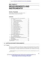
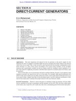
FIGURE 18-1 Typical distribution system.
18.1 DISTRIBUTION DEFINED
Broadly speaking, distribution includes all parts of an electric utility system between bulk power
sources and the consumers’ service-entrance equipments. Some electric utility distribution engineers,
however, use a more limited definition of distribution as that portion of the utility system between the
distribution substations and the consumers’ service-entrance equipment. In general, a typical distrib-
ution system consists of (1) subtransmission circuits with voltage ratings usually between 12.47 and
345 kV which deliver energy to the distribution substations, (2) distribution substations which convert

the energy to a lower primary system voltage for local distribution and usually include facilities for
voltage regulation of the primary voltage, (3) primary circuits or feeders, usually operating in the
range of 4.16 to 34.5 kV and supplying the load in a well-defined geographic area, (4) distribution
transformers in ratings from 10 to 2500 kVA which may be installed on poles or grade-level pads or
in underground vaults near the consumers and transform the primary voltages to utilization voltages,
(5) secondary circuits at utilization voltage which carry the energy from the distribution transformer
along the street or rear-lot lines, and (6) service drops which deliver the energy from the secondary
to the user’s service-entrance equipment. Figures 18-1 and 18-2 depict the component parts of a typ-
ical distribution system.
Distribution investment constitutes 50% of the capital investment of a typical electric utility sys-
tem. Recent trends away from generation expansion at many utilities have put increased emphasis
on distribution system development.
The function of distribution is to receive electric power from large, bulk sources and to distribute
it to consumers at voltage levels and with degrees of reliability that are appropriate to the various
types of users.
For single-phase residential users, American National Standard Institute (ANSI) C84.1-1989
defines Voltage Range A as 114/228 V to 126/252 V at the user’s service entrance and 110/220 V to
126/252 V at the point of utilization. This allows for voltage drop in the consumer’s system. Nominal
voltage is 120/240 V. Within Range A utilization voltage, utilization equipment is designed and rated
to give fully satisfactory performance.
As a practical matter, voltages above and below Range A do occur occasionally; however, ANSI
C84.1 specifies that these conditions shall be limited in extent, frequency, and duration. When they
do occur, corrective measures shall be undertaken within a reasonable time to improve voltages to
meet Range A requirements.
Rapid dips in voltage which cause incandescent-lamp “flicker” should be limited to 4% or 6%
when they occur infrequently and 3% or 4% when they occur several times per hour. Frequent dips,
such as those caused by elevators and industrial equipment, should be limited to 1
1
/
2

% or 2%.
Beaty_Sec18.qxd 17/7/06 8:53 PM Page 18-2
Downloaded from Digital Engineering Library @ McGraw-Hill (www.digitalengineeringlibrary.com)
Copyright © 2006 The McGraw-Hill Companies. All rights reserved.
Any use is subject to the Terms of Use as given at the website.
POWER DISTRIBUTION
POWER DISTRIBUTION 18-3
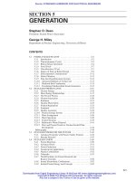
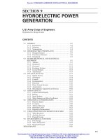
FIGURE 18-2 One-line diagram of typical primary distribution feeder.
Reliability of service can be described by factors such as frequency and duration of service inter-
ruptions. While short and infrequent interruptions may be tolerated by residential and small com-
mercial users, even a short interruption can be costly in the case of many industrial processes and
can be dangerous in the case of hospitals and public buildings. For such sensitive loads, special mea-
sures are often taken to ensure an especially high level of reliability, such as redundancy in supply
circuits and/or supply equipment. Certain computer loads may be sensitive not only to interruptions
but even to severe voltage dips and may require special power-supply systems which are virtually
uninterruptible.
From a system-planning and design point of view, the optimal choice of subtransmission voltage
and system arrangement is closely interrelated with distribution substation size and with the primary
distribution voltage level. At any given time, the most economical arrangement is achieved when the
sum of the subtransmission, substation, and primary feeder costs to serve an area is a minimum over
Beaty_Sec18.qxd 17/7/06 8:53 PM Page 18-3
Downloaded from Digital Engineering Library @ McGraw-Hill (www.digitalengineeringlibrary.com)
Copyright © 2006 The McGraw-Hill Companies. All rights reserved.
Any use is subject to the Terms of Use as given at the website.
POWER DISTRIBUTION
18-4 SECTION EIGHTEEN
*
From “Out of Sight, Out of Mind?,” January 2004, Edison Electric Institute (used with permission).
the life of the facilities. In practice, the number, size, and availability of bulk supply sources for feed-
ing the subtransmission may be significant factors as well.

A distribution system should be designed so that anticipated load growth can be served at mini-
mum expense. This flexibility is needed to handle load growth in existing areas as well as load
growth in new areas of development.
Overhead and underground distribution systems are both used in large metropolitan areas. In the
past in smaller towns and in the less-congested areas of larger cities, overhead distribution was
almost universally used; the cost of underground distribution for residential areas was several times
that of overhead. During the past 25 to 30 years, the cost of underground residential distribution
(URD) has been reduced drastically through the development of low-cost, solid-dielectric cables
suitable for direct burial, mass production of pad-mounted distribution transformers and accessories,
mechanized cable-installation methods, etc. The cost of a typical URD system for a new residential
subdivision is about 50% greater than that of an overhead system in many areas; in others, there is
little or no differential due to local land conditions. As a result, some utilities will justifiably have
some type of extra charge for underground. With the increased public interest in improving the
appearance of residential areas and the declining cost of URD, the growth of URD has been
extremely rapid. Today, perhaps as much as 70% of new residential construction is served under-
ground. A number of states have enacted legislation making underground distribution mandatory for
new residential subdivisions.
Undergrounding
*
. In the last decade, U.S. East Coast and Midwest regions experienced several
catastrophic “100 year storms.” These storms left widespread electric power outages that lasted sev-
eral days. Given the critical role that electricity plays in our modern lifestyle, even a momentary
power outage is an inconvenience. A days-long power outage presents a major hardship and can be
catastrophic in terms of its health and safety consequences, and the economic losses it creates. Why
then, don’t we bury more of our power lines so they will be protected from storms?
The fact is we already are placing significant numbers of power lines underground. Over the past
10 years, approximately half of the capital expenditures by U.S. investor-owned utilities for new
transmission and distribution wires have been for underground wires. Almost 80% of the nation’s
electric grid, however, has been built with overhead power lines. Would electric reliability be
improved if more of these existing overhead lines were placed underground as well?

What the report finds is that burying existing overhead power lines does not completely protect
consumers from storm-related power outages. However, underground power lines do result in fewer
overall power outages, but the duration of power outages on underground systems tends to be longer
than for overhead lines. Also, undergrounding is expensive, costing up to $1 million/mile or almost
10 times the cost of a new overhead power line. This means that most undergrounding projects can-
not be economically justified and must cite intangible, unquantifiable benefits such as improved
community or neighborhood aesthetics for their justification. Determining who pays and who bene-
fits from undergrounding projects can be difficult and often requires the establishment of separate
government-sponsored programs for funding.
How Much Does Undergrounding Improve Electric Reliability? Comparative reliability data
indicate that the frequency of outages on underground systems can be substantially less than for over-
head systems. However, when the duration of outages is compared, underground systems lose much
of their advantage. The data show that the frequency of power outages on underground systems is only
about one-third of that of overhead systems. A 2000 report issued by the Maryland Public Service
Commission concluded that the impact of undergrounding on reliability was “unclear.”
In a 2003 study, the North Carolina Commission summarized 5 years of underground and over-
head reliability comparisons for North Carolina’s investor-owned electric utilities–Dominion North
Carolina Power, Duke Energy, and Progress Energy Carolinas. The data indicate that the frequency
of outages on underground systems was 50% less than for overhead systems, but the average
duration of an underground outage was 58% longer than for an overhead outage. In other words, for
Beaty_Sec18.qxd 17/7/06 8:53 PM Page 18-4
Downloaded from Digital Engineering Library @ McGraw-Hill (www.digitalengineeringlibrary.com)
Copyright © 2006 The McGraw-Hill Companies. All rights reserved.
Any use is subject to the Terms of Use as given at the website.
POWER DISTRIBUTION
POWER DISTRIBUTION 18-5
the North Carolina utilities, an underground system suffers only about half the number of outages of
an overhead system, but those outages take 1.6 times longer to repair. Based on this data, Duke
Power concluded, “Underground distribution lines will improve the potential for reduced outage
interruption during normal weather, and limit the extent of damage to the electrical distribution sys-

tem from severe weather-related storms.” However, once an interruption has occurred, underground
outages normally take significantly longer to repair than a similar overhead outage.
Reliability Characteristics of Overhead and Underground Power Lines
• Overhead lines tend to have more power outages primarily due to trees coming in contact with
overhead lines.
• It is relatively easy to locate a fault on an overhead line and repair it. A single line worker, for
example, can locate and replace a blown fuse. This results in shorter duration outages.
• Underground lines require specialized equipment and crews to locate a fault, a separate crew with
heavy equipment to dig up a line, and a specialized crew to repair the fault. This greatly increases
the cost and the time to repair a fault on an underground system.
• In urban areas, underground lines are 4 times more costly to maintain than overhead facilities.
• Underground lines have a higher failure rate initially due to dig-ins and installation problems. After
3 or 4 years, however, events that affect failures become virtually nonexistent.
• As underground cables approach their end of life, failure rates increase significantly and these failures
are extremely difficult to locate and repair. Maryland utilities report that their underground cables are
becoming unreliable after 15 to 20 years and reaching their end of life after 25 to 35 years.
• Pepco found that customers served by 40-year-old overhead lines had better reliability than cus-
tomers served by 20-year-old underground lines.
• Two Maryland utilities have replaced underground distribution systems with overhead systems to
improve reliability.
• Water and moisture infiltration can cause significant failures in underground systems when they
are flooded, as often happens in hurricanes.
• Due to cost or technical considerations, it is unlikely that 100% of the circuit from the substation
to the customer can be placed entirely underground. This leaves the circuit vulnerable to the same
types of events that impact other overhead lines, for example, high winds and ice storms.
Other Benefits of Undergrounding. One of the most commonly cited benefits of undergrounding
is the removal of unsightly poles and wires. Local communities and neighborhoods routinely spend
millions to place their existing overhead power lines underground.
Similarly, when given the option, builders of new residential communities will often pay a pre-
mium of several thousand dollars/home to place the utilities underground. These “aesthetic” benefits

are virtually impossible to quantify, but are, in many instances, the primary justification for projects
to place existing power lines underground.
Underground lines do have other benefits. In 1998, Australia completed a major benefit/cost
analysis of undergrounding all existing power lines in urban and suburban areas throughout the coun-
try. The study costed more than $1.5 million Australian ($1.05 million U.S. at current rates), and rep-
resents what may be the most comprehensive undertaking to date to quantify the benefits and costs
related to undergrounding.
In addition to the value of improved aesthetics, the study identified the following potential bene-
fits related to undergrounding that it attempted to quantify:
• Reduced motor vehicle accidents caused by collisions with poles
• Reduced losses caused by electricity outages
• Reduced network maintenance costs
• Reduced tree-pruning costs
Beaty_Sec18.qxd 17/7/06 8:53 PM Page 18-5
Downloaded from Digital Engineering Library @ McGraw-Hill (www.digitalengineeringlibrary.com)
Copyright © 2006 The McGraw-Hill Companies. All rights reserved.
Any use is subject to the Terms of Use as given at the website.
POWER DISTRIBUTION
18-6 SECTION EIGHTEEN
• Increased property values
• Reduced transmission losses due to the use of larger conductors
• Reduced greenhouse-gas emissions (lower transmission losses)
• Reduced electrocutions
• Reduced brushfire risks, and
• Indirect effects on the economy such as employment
Of this list, the only four items deemed significant in the study’s benefit/cost calculations included:
• Motor vehicle accidents
• Maintenance costs
• Tree-trimming costs, and
• Line losses

The Australian list of benefits does not include improved reliability as a significant benefit of
undergrounding. Instead it identifies the reduction in losses from motor vehicle accidents as the
largest benefit from undergrounding—something utilities have no control over.
Underground cost data for U.S. utilities indicate that the cost of placing overhead power lines
underground is 5 to 10 times the cost of new overhead power lines. Other factors also can result in
substantial additional customer costs for undergrounding projects. These include:
• Electric undergrounding strands other utilities, for example, cable and telephone companies, which
must assume 100% of pole costs if electric lines are underground. These additional nonelectric
costs will likely be passed on to cable and telephone consumers.
• Customers may incur substantial additional costs to connect homes to newly installed underground
service, possibly as much as $2000 if the household electric service must be upgraded to conform
to current electric codes.
Paying for Undergrounding. In spite of its high cost and lack of economic justification, under-
grounding is very popular across the country. In 9 out of 10 new subdivisions, contractors bury power
lines. In addition, dozens of cities have developed comprehensive plans to bury or relocate utility
lines to improve aesthetics.
For new residential construction, utilities vary on how they charge for the cost of providing
underground services. When it comes to converting existing overhead lines to underground, a vari-
ety of programs are being utilized. They include special assessment areas, undergrounding districts,
and state and local government initiatives.
Placing existing power lines underground is expensive, costing approximately $1 million/mile.
This is almost 10 times the cost of a new overhead power line.
While communities and individuals continue to push for undergrounding—particularly after
extended power outages caused by major storms—the reliability benefits that would result are uncer-
tain, and there appears to be little economic justification for paying the required premiums.
Indeed, in its study of the undergrounding issue, the Maryland Public Service Commission con-
cluded, “If a 10 percent return is imputed to the great amounts of capital freed up by building over-
head instead of underground lines, the earnings alone will pay for substantial ongoing overhead
maintenance,” implying that utilities could have more resources available to them to perform main-
tenance and improve reliability on overhead lines if they invested less in new underground facilities.

For the foreseeable future, however, it appears that the undergrounding of existing overhead power
lines will continue, justified primarily by aesthetic considerations—not reliability or economic bene-
fits. Many consumers simply want their power lines placed underground, regardless of the costs. The
challenge for decision makers is determining who will pay for these projects and who will benefit.
There are several undergrounding programs around the country that are working through these
equity issues and coming up with what appear to be viable compromises. Once a public-policy
Beaty_Sec18.qxd 17/7/06 8:53 PM Page 18-6
Downloaded from Digital Engineering Library @ McGraw-Hill (www.digitalengineeringlibrary.com)
Copyright © 2006 The McGraw-Hill Companies. All rights reserved.
Any use is subject to the Terms of Use as given at the website.
POWER DISTRIBUTION
POWER DISTRIBUTION 18-7
decision is reached to pursue an undergrounding project, it is worthwhile for the leaders involved
to evaluate these programs in more detail to determine what is working, and what is not.
Rural Service. Rural service has been extended to most farmers and rural dwellers through
the efforts of utilities, cooperatives, and government agencies. Rural construction must be of the
least-expensive type consistent with durability and reliability because there may be only a
few users per mile of line. Historically, rural construction has been overhead, but the advent of
cable-plowing techniques has made underground economically competitive with overhead in some
parts of the country, and a growing amount of rural distribution is being installed underground.
Higher primary voltages of 24.9Y/14.4 and 34.5Y/19.92 kV are continuing to grow in usage,
although primary voltages in the 15-kV class predominate. The 5-kV class continues to decline in
usage. Surveys indicate that in recent years approximately 78% of the overhead and underground
line additions are at 15 kV, 11% are at 25 kV, and 7.5% are at 35 kV.
Generally, when a higher distribution voltage is initiated, it is built in new, rapidly growing
load areas. The economic advantage of the higher voltages usually is not great enough to justify
massive conversions of existing lower-voltage facilities to the higher level. The lower-voltage
areas are contained and gradually compressed over a period of years as determined by economics,
obsolescence, and convenience. Virtually, all modern primary systems serving residential and
small commercial and small industrial loads are 4-wire, multigrounded, common-neutral systems.

18.2 DISTRIBUTION-SYSTEM AUTOMATION
Distribution automation (DA), a system to monitor and control the distribution system in real-time,
was gradually introduced in the 1970s more as a concept than a fully developed plan. Unlike the
introduction of EMS, where utilities readily saw the benefits of automatic generation control and
economic dispatch and adopted the technology, utilities were much more cautious in their approach
to distribution automation.
Early distribution automation projects were undertaken by a handful of utilities. The technology
was changing and evolving so much so that DA was being touted as an amorphous system capable
of covering any imaginable function under the sun. A 1984 EPRI project, Guidelines for Evaluating
Distribution Automation, focused attention on what functions could be automated and what value
could be attached to those functions. A positive result of this project is that it got people thinking
about what functions mattered most. However, it was a little bit ahead of its time in that there wasn’t
much standardization in systems employed for DA and one couldn’t simply select functions of inter-
est and expect to obtain a system that could be built for the total value of the functions selected. Then
too, the choice of the communications systems (e.g., telephone, fiber optics, radio, carrier, etc.)
proved to be a barrier to widespread implementation.
At the substation level, equipment loadings became an early focus, and asset management became
a desired function for DA systems. In addition, the ability to trip distribution circuit breakers and
transfer load between substations was commonplace as SCADA was added and this represented the
extent of distribution automation to many companies.
Volt/var control, that is, controlling the combination of load tap changers (LTC) or voltage regu-
lators and switched capacitor banks within a substation, was a function many companies incorpo-
rated with DA. With adoption of microprocessor relays and fault distance relaying, some incorporated
the output information from fault distance relays and diagnostic alarms from various subsystems to
be part of the DA package.
Moving outside the substation, controlling automated circuit tie switches was prompted by reli-
ability considerations. Having SCADA links to other reclosers, particularly the ones with micro-
processor controls, enabled more ability to remotely control field switching and achieve more rapid
restoration of service.
Distribution automation is still evolving with systems incorporating many of the functions previ-

ously described. More utilities are employing varying degrees of distribution automation and more
standardization is taking place.
Beaty_Sec18.qxd 17/7/06 8:53 PM Page 18-7
Downloaded from Digital Engineering Library @ McGraw-Hill (www.digitalengineeringlibrary.com)
Copyright © 2006 The McGraw-Hill Companies. All rights reserved.
Any use is subject to the Terms of Use as given at the website.
POWER DISTRIBUTION
18-8 SECTION EIGHTEEN
18.3 CLASSIFICATION AND APPLICATION
OF DISTRIBUTION SYSTEMS
Distribution systems may be classified in according to:
• voltage—120 V, 12,470 V, 34,500 V, etc.
• scheme of connection—radial, loop, network, multiple, and series.
• loads—residential, small light and power, large light and power, street lighting, railways, etc.
• number of conductors—2-wire, 3-wire, 4-wire, etc.
• type of construction—overhead or underground.
• number of phases—single-phase, 2-phase, or 3-phase; and as to frequency: 25 Hz, 60 Hz, etc.
Application of Systems. In American practice, alternating-current (ac) 60-Hz systems are almost
universally used for electric power distribution. These systems comprise the most economical
method of power distribution, owing in large measure to the ease of transforming voltages to levels
appropriate to the various parts of the system. These transformations are accomplished by means of
reliable and economical transformers. By proper system design and the application of overvoltage
and overcurrent protective equipment, voltage levels and service reliability can be matched to almost
any consumer requirement.
Single-phase residential loads generally are supplied by simple radial systems at 120/240 V. The
ultimate in service reliability is provided in densely loaded business/commercial areas by means of
grid-type secondary-network systems at 208Y/120 V or by “spot” networks, usually at 480Y/277 V.
Secondary-network systems are used in about 90% of the cities in this country having a population of
100,000 or more and in more than one-third of all cities with populations between 25,000 and 100,000.
Where secondary-network systems do not supply sufficiently reliable service for critical loads,

emergency generators and/or batteries are sometimes provided together with automatic switching
equipment so that service can be maintained to the critical loads in the event that the normal utility sup-
ply is interrupted. Such loads are found in hospitals, computer centers, key industrial processes, etc.
Single-phase residential loads are almost universally supplied through 120/240-V, 3-wire, single-
phase services. Large appliances, such as ranges, water heaters, and clothes dryers, are served at 240
V. Lighting, small appliances, and convenience outlets are supplied at 120 V.
An exception to the preceding comments occurs when the dwelling unit is in a distributed
secondary-network area served at 280Y/120 V. In this case, large appliances are supplied at 208 V
and small appliances at 120 V.
Three-phase, 4-wire, multigrounded, common-neutral primary systems, such as 12.47Y/7.2 kV, 24.9Y/
14.4 kV, and 34.5Y/19.92 kV, are used almost exclusively. The fourth wire of these Y-connected
systems is the neutral for both the primary and the secondary systems. It is grounded at many loca-
tions. Single-phase loads are served by distribution transformers, the primary windings of which are
connected between a phase conductor and the neutral. Three-phase loads can be supplied by 3-phase
distribution transformers or by single-phase transformers connected to form a 3-phase bank. Primary
systems in the 15-kV class are most commonly used, but the higher voltages are gaining acceptance.
Figure 18-2 illustrates a typical radial primary feeder.
The 4-wire system is particularly economic for URD systems because each primary lateral or
branch circuit consists of only one insulated phase conductor and the bare, uninsulated neutral rather
than two insulated conductors. Also, only one primary fuse is required at each transformer and one
surge arrester in overhead installations.
Three-phase, 3-wire primary systems are not widely used for public distribution, except in
California. They can be used to supply single-phase loads by means of distribution transformers having
primary winding connected between two phase conductors. Single-phase primary laterals consist of
two insulated phase conductors; each single-phase distribution transformer requires two fuses and
two surge arresters (where used). Three-phase loads are served through 3-phase distribution trans-
formers or appropriate 3-phase banks. Two-phase systems are rarely used today.
Beaty_Sec18.qxd 17/7/06 8:53 PM Page 18-8
Downloaded from Digital Engineering Library @ McGraw-Hill (www.digitalengineeringlibrary.com)
Copyright © 2006 The McGraw-Hill Companies. All rights reserved.

Any use is subject to the Terms of Use as given at the website.
POWER DISTRIBUTION
POWER DISTRIBUTION 18-9
18.4 CALCULATION OF VOLTAGE REGULATION AND I
2
R LOSS
When a circuit supplies current to a load, it experiences a drop in voltage and a dissipation of energy
in the form of heat. In dc circuits, voltage drop is equal to current in amperes multiplied by the resis-
tance of the conductors, V ϭ IR. In ac circuits, voltage drop is a function of load current and power
factor and the resistance and reactance of the conductors. Heating is caused by conductor losses; for
both dc and ac circuits they are computed as the square of current multiplied by conductor resistance
in ohms. Watts ϭ I
2
R, or kW ϭ I
2
R/1000. Capacitance can usually be neglected for calculation in
distribution circuits because its effect on voltage drop is negligible for the circuit lengths and oper-
ating voltages used. In circuit design, a conductor size should be selected so that it will carry the
required load within specified voltage-drop limits and will have an optimized value of installed cost
and cost of losses. Today, a conductor size meeting these criteria will operate well within safe oper-
ating temperature limits. In some cases, short-circuit current requirements will dictate the minimum
conductor size.
Percent voltage drop or percent regulation is the ratio of voltage drop in a circuit to voltage deliv-
ered by the circuit, multiplied by 100 to convert to percent. For example, if the drop between a trans-
former and the last customer is 10 V and the voltage delivered to the customer is 240, the percent
voltage drop is 10/240 ϫ 100 ϭ 4.17%. Often the nominal or rated voltage is used as the denomi-
nator because the exact value of delivered voltage is seldom known.
Percent I
2
R or percent conductor loss of a circuit is the ratio of the circuit I

2
R or conductor loss,
in kilowatts, to the kilowatts delivered by the circuit (multiplied by 100 to convert to percent). For
example, assume a 240-V single-phase circuit consisting of 1000 ft of two No. 4/0 copper cables
supplies a load of 100 A at unity power factor.
Direct-current voltage drop is easily calculated by multiplying load amperes I by ohmic resis-
tance R of the conductors through which the current flows (see Sec. 4 for ohmic resistance of vari-
ous conductors).
Example: A 500-ft dc circuit of two 4/0 copper cables carries 200 A. What is the voltage drop?
Resistance of 1000 ft of 4/0 copper cable is 0.0512 ⍀.
If 240 is the delivered voltage,
I
2
R or conductor loss in dc or ac circuits is calculated by multiplying the square of the current in
amperes by ohmic resistance of the conductors through which the current flows. The result is in watts.
In dc circuits, percent voltage drop and percent conductor loss are identical.
In ac circuits, the ratio of percent conductor loss to percent voltage regulation is given approximately
by the following approximate formula:
(18-1)
where ␪ ϭ power-factor angle and ␾ ϭ impedance angle; that is, tan ␾ ϭ X/R.
% I
2
R loss
% voltage drop
ϭ
cos
f
cos u cos (f Ϫ u)
% I
2

R ϭ I
2
R/VI ϫ 100 ϭ IR/V ϫ 100
% voltage drop ϭ IR/V ϫ 100
% regulation ϭ 10.24/240 ϫ 100 ϭ 4.26%
Drop ϭ IR ϭ 200 ϫ 0.0512 ϭ 10.24 V
% I
2
R loss ϭ 1.024/24 ϫ 100 ϭ 4.26%
Load delivered ϭ 240 ϫ 100 ϭ 24,000 W ϭ 24 kW
I
2
R ϭ 100
2
ϫ 2 ϫ 0.0512 ϭ 1024 W ϭ 1.024 kW
Beaty_Sec18.qxd 17/7/06 8:53 PM Page 18-9
Downloaded from Digital Engineering Library @ McGraw-Hill (www.digitalengineeringlibrary.com)
Copyright © 2006 The McGraw-Hill Companies. All rights reserved.
Any use is subject to the Terms of Use as given at the website.
POWER DISTRIBUTION
18-10 SECTION EIGHTEEN
TABLE 18-1 Voltage Drop in Volts per 100,000 A ⋅ ft,
2-Wire DC Circuits (Loop)
Conductor size, AWG or kcmil
Approx. equivalent
Copper aluminum
6 4 102.8
4 2 64.6
2 1/0 40.7
1/0 3/0 25.6

2/0 4/0 20.3
4/0 336 12.8
350 556 7.71
500 795 5.39
1000 2.70
1500 1.80
2000 1.35
Note: 1 ft ϭ 0.3048 m.
Volts drop per
100,000 A ⋅ ft,
90º copper temp
Table 18-1 gives voltage drop in volts per 100,000 A ⋅ ft for 2-wire dc circuits for a number of
conductor sizes. Ampere-feet is the product of the number of amperes of current flowing and the dis-
tance in feet between the sending and receiving terminals multiplied by 2 to take into account the
drop in both the outgoing and return conductors. Or the feet can be considered to be the total num-
ber of conductor feet, outgoing and return.
Table 18-1 also gives the voltage drop for 3-wire circuits when serving balanced loads, where the
term “feet” is taken to mean twice the number of feet between sending and receiving terminals.
Example 1. What is the voltage drop and percent voltage drop when 200 A dc flows 1500 ft one
way through a 2-wire, 120-V, 556-kcmil aluminum circuit? First determine ampere-feet factor as
100 ϫ 1500/100,000 ϭ 1.5. From Table 18-1, the voltage drop is 7.71 V per 100,000 A ⋅ ft. This
value multiplied by the 1.5 factor gives the total voltage drop ϭ 1.5 ϫ 7.71 ϭ 11.6 V. The percent
voltage drop ϭ 11.6 ϫ 100/120 ϭ 9.64%. The percent conductor loss also is 9.64%, which is
equivalent to 120 ϫ 100 ϫ 0.0954 ϭ 1.16 kW.
Example 2. A mine 1 mile from a motor-generator station must receive 100 kW dc at not less
than 575 V. Maximum voltage of the generator is 600 V. What conductor size should be used?
18.36 ϫ voltage drop per 100,000 A ⋅ ft from Table 18-1 ϭ 25 V
Therefore, voltage drop per 100,000 A ⋅ ft ϭ 25/18.36 ϭ 1.36. From Table 18-1, the copper con-
ductor size corresponding to 1.36 V/100,000 A ⋅ ft is 2000 kcmil copper.
Calculating Voltage Drop in AC Circuits. The voltage drop per mile in each round wire of 3-phase

60-Hz line with equilateral spacing D inches between centers or in each wire of a single-phase line
D inches between centers is
(18-2)V
~
drop ϭ I
~
R ϩ jI
~
a0.2794 log
D
r
ϩ 0.03034 mb

volts in phasor form
A
#
ft
100,000
ϭ
173.9 ϫ 10,560
100,000
ϭ 18.36
Loop ft ϭ 2 ϫ 5280 ϭ 10,560 ft
Max. current ϭ
100,000 W
575 V
ϭ 173.9 A
Beaty_Sec18.qxd 17/7/06 8:53 PM Page 18-10
Downloaded from Digital Engineering Library @ McGraw-Hill (www.digitalengineeringlibrary.com)
Copyright © 2006 The McGraw-Hill Companies. All rights reserved.

Any use is subject to the Terms of Use as given at the website.
POWER DISTRIBUTION
POWER DISTRIBUTION 18-11
where is in phasor amperes, R is the 60-Hz resistance of the wire per mile, ⍀, log is the log to
base 10, r is the radius of round wire, in, and µ is the permeability of the wire (unity for nonmag-
netic materials such as copper or aluminum). j in Eq. (18-2) denotes an angle of 90Њ; ϩ j means 90Њ
leading, Ϫj means 90Њ lagging. Thus, the expression for phasor current lagging the reference volt-
age is with reference to a conveniently chosen horizontal axis of reference—usu-
ally sending- or receiving-end voltage. The symbol ϳ over I or V indicates phasor values. Voltage
drops determined in this manner are also phasors and are with respect to the reference axis.
When wire is stranded, an equivalent radius must be used for r in Eq. (18-2). r ϭ 0.528 for
7 strands, r ϭ 0.5585 for 19 strands, r ϭ 0.5675 for 37 strands, where r ϭ equivalent
radius, in, and A ϭ area of metal, in
2
.
Frequency is 60 Hz for the constants in parentheses in Eq. (18-2), which gives reactance X in
ohms per mile. For 25 Hz, multiply by 25/60. The equation is sometimes written
(18-3)
where I is in phasor amperes and Z ϭ Z/␾ ⋅ ⍀/mi at 60 Hz.
Three unsymmetrically spaced wires a, b, and c of a 3-phase circuit with correct transpositions
can have voltage drop in each wire calculated by Eq. (18-2) by substituting for D the geometric mean
of the three interaxial distances:
The Phasor Method. In Eq. (18-3), I is in vector amperes,
where ␪ is the angle that the current lags (or
leads) the voltage. The sending-end voltage is
usually chosen as the axis, or phasor, of
reference in drawing the phasor diagram.
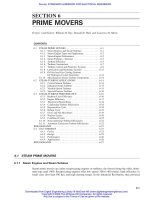
For example, consider Fig. 18-3, where sending
voltage , load current I ϭ I , circuit
impedance ϭ Z ϭ R ϩ jX, and load

voltage (all phasors). The
symbol is used for positive angles, assum-
ing that the counterclockwise direction from
the phasor or reference is positive and the clockwise directions negative. Assume that V
s
ϭ 230/0Њ,
ϭ 50 , ϭ 0.2 , and ϭ R ϩ jX. Thus
ϫ 0.2
ϭ 230 Ϫ 10
ϭ 230 Ϫ 10 cos 34.70ЊϪj 10 sin 34.70Њ
ϭ 230 Ϫ 8.22 Ϫ j 5.69 ϭ 221.78 Ϫ j 5.69
ϭ 221.78 (very nearly)
Neglecting the term Ϫj 5.69 simplifies the final calculation and gives the load voltage within a
fraction of 1% of the precise result. This method is sufficiently accurate for practically all distribu-
tion engineering calculations and can be thought of as
(18-4) V drop ϭ IR cos u ϩ IX sin u ϭ IZ cos (f Ϫ u)
>
34.70
Њ
>
uЊ
>
71.57Њ
>
36.87Њ
V
~
L
ϭ 230/0ЊϪ50
Z

~
>
71.57Њ
Z
~
>
Ϫ36.87Њ
I
~
l
V
~
L
ϭ V
~
s
Ϫ I
~
Z
~
>
uЊ
Z
~
>
uЊ
>
uЊ
V
s

ϭ V
s
I
~
ϭ I
x
Ϫ jI
y
ϭ I
l
u
D ϭ 2
3
D
ab
D
bc
D
ca
V
~
drop per mile ϭ I
~
(R ϩ jX) ϭ I
~
Z
~
volts in phasor form
!A
!A

!A
I
~
ϭ I
x
Ϫ jI
y
ϭ I!uЊ
I
~
FIGURE 18-3 Phasor diagram showing voltage relationships.
Beaty_Sec18.qxd 17/7/06 8:53 PM Page 18-11
Downloaded from Digital Engineering Library @ McGraw-Hill (www.digitalengineeringlibrary.com)
Copyright © 2006 The McGraw-Hill Companies. All rights reserved.
Any use is subject to the Terms of Use as given at the website.
POWER DISTRIBUTION
18-12 SECTION EIGHTEEN
where I and Z are absolute magnitudes, not phasor quantities, ␾ is the impedance angle, and ␪ is the
power-factor angle by which the current lags (or leads) the voltage. Calculating the drop in the above
example by this method:
or
Impedance Z can be visualized as the hypotenuse of a
right triangle in which the base is the resistance R and the
altitude is the reactance X. In phasor form,
˜
Z ϭ R Ϯ jX,
where the positive sign is used for inductive reactance
and the negative sign for capacitive reactance. Impedance
also can be expressed as
˜

Z ϭ Z , where Z is the
absolute magnitude and ␾ is the angle between
˜
Z and R in
Fig. 18-4. This angle is an absolute value in that it has no
relationship to the axis of reference in a phasor diagram,
as do voltage and current. Alternating current causes a
voltage drop in resistance which is in time phase with
the current and in inductive reactance a drop which
leads the current by 90 electrical degrees, assuming the
positive direction for measurement of angles is counter-
clockwise. Or conversely, the current in an inductive
reactance lags the voltage drop by 90Њ.
Impedance Values. Tables are available which give
60-Hz impedance values in ohms per 1000 ft for com-
mon sizes of wire and cable. The values can be
expressed in the form
˜
Z ϭ R ϩ jX, which can be
converted to the form Z if desired. The latter form is
convenient to use in voltage-drop calculations when the
current is expressed as I .
Power Factor. In typical distribution loads, the current
lags the voltage, as shown in Fig. 18-3, where ␪ is shown as the angle between current and sending
voltage and cos ␪ is referred to as the power factor of the circuit. In a purely resistive circuit, the cur-
rent and voltage are in phase; consequently, the power factor is 1.0 or unity. In a purely inductive
circuit, the voltage and current are out of phase by 90 electrical degrees, resulting in a power factor
of zero. In a circuit consisting of a resistance in series with a reactance of equal ohmic value (␾ ϭ 45Њ),
␪ ϭϮ45Њ also. Thus, the power factor is cos 45Њϭ0.707, or 70.7%.
In a single-phase ac circuit, the load in kW can be expressed as

kW ϭ EI cos ␪ (18-5)
where Eϭ magnitude of rms line-to-neutral voltage, kV
Iϭmagnitude of current, rms amperes
␪ϭelectrical angle between phasor voltage and current
>fЊ
>fЊ
>fЊ
ϭ 10 cos (34.7Њ) ϭ 10 ϫ 0.822 ϭ 8.22 V
V drop ϭ IZ cos (f Ϫ u) ϭ 50 ϫ 0.2 ϫ cos (71.57ЊϪ36.87Њ)
ϭ 2.53 ϩ 5.69 ϭ 8.22 V
ϩ 50 ϫ 0.2 ϫ sin 71.57Њ ϫ sin 36.87Њ
V drop ϭ 50 ϫ 0.2 ϫ cos 71.57Њ ϫ cos 36.87Њ
FIGURE 18-4 Impedance diagrams for series
connection of resistance and reactance (L ϭ
inductance, in henrys; C ϭ capacitance, in farads;
F ϭ frequency, in hertz).
Beaty_Sec18.qxd 17/7/06 8:53 PM Page 18-12
Downloaded from Digital Engineering Library @ McGraw-Hill (www.digitalengineeringlibrary.com)
Copyright © 2006 The McGraw-Hill Companies. All rights reserved.
Any use is subject to the Terms of Use as given at the website.
POWER DISTRIBUTION
POWER DISTRIBUTION 18-13
From Eq. (18-5), it is obvious that the magnitude of the current for a given voltage and kilowatt
load depends on the power factor, or
I ϭ kW/(E cos ␪) (18-6)
The corresponding equations for balanced 3-phase circuits are
kW ϭ EI cos ␪ (18-7)
and
I ϭ kW/( E cos ␪) (18-8)
where the symbols are as specified above, and ␪ is measured as the angle between the line-to-

neutral voltage of a given phase and the current in that phase.
Example. Given a load of 500 kW at 80% power factor (lagging), 7.2 kV circuit voltage, 60-Hz,
single-phase circuit using 1/0 aluminum conductor spaced 30 in on centers. The load is located 1 mi
from the substation. What is the voltage drop? From tables on conductor characteristics,
r ϭ 0.185 ⍀/1000 ft
x ϭ 0.124 ⍀/1000 ft
Therefore, R ϩ jX ϭ 5.28 (0.185 ϩ j 0.124) ϭ 0.9769 ϩ j 0.6547 ⍀
From Eq. (18-6),
E ϭ 7.2
cos ␪ ϭ 0.80
␪ ϭ 36.87Њ
and sin ␪ ϭ 0.60
From Eq. (18-4),
*
Calculation of 3-Phase Line Drops with Balanced Loads. In 3-phase circuits with balanced loads
on each phase, the line-to-neutral voltage drop is merely the product of the phase current and the con-
ductor impedance as determined from standard tables. There is no return current with balanced
3-phase loads. Thus, the line-to-line voltage drop is times the line-to-neutral drop, or
(18-9) V
drop LϪL
ϭ 23(IR cos u ϩ IX sin u)
!3
ϭ 2(67.84 ϩ 34.10) ϭ 203.88 V
Voltage drop ϭ 2(IR cos u ϩ IX sin u) ϭ (86.81 ϫ 0.9769 ϫ 0.8 ϩ 86.81 ϫ 0.6547 ϫ 0.6)
>
uЊ
I ϭ
kW
E cos u
ϭ

500
7.2 ϫ 0.8
ϭ 86.81 A
!3
!3
*The factor of 2 is used for a single-phase system to represent the impedance of the outgoing conductor and the return
conductor.
Beaty_Sec18.qxd 17/7/06 8:53 PM Page 18-13
Downloaded from Digital Engineering Library @ McGraw-Hill (www.digitalengineeringlibrary.com)
Copyright © 2006 The McGraw-Hill Companies. All rights reserved.
Any use is subject to the Terms of Use as given at the website.
POWER DISTRIBUTION
18-14 SECTION EIGHTEEN
For example, assume that the circuit of the preceding example now is a 3-phase 12.47-kV circuit
1 mi long with the same 1/0 aluminum conductors at an equivalent spacing of 30 in and a load of
3 ϫ 500 ϭ 1500 kW at 0.8 pf lagging. What is the line-to-line voltage drop? R and X are the same
values as previously; that is, R ϩ jX ϭ 0.9769 ϩ j 0.6547 ⍀.
The current per phase from Eq. (18-7) is
as before,
Calculation of Voltage Drop in Unbalanced Unsymmetrical Circuits. If there are n different wires
a, b, c, d, ⋅ ⋅ ⋅ , n carrying currents I
a
, I
b
, I
c
, ⋅ ⋅ ⋅ , I
n
, respectively, whether 2-, 3-phase, the voltage
drop in wire a per mile at 60 Hz is

(18-10)
where currents are in phasor amperes, R
a
is 60-Hz ohmic resistance of conductor a per mile, r is
equivalent radius, in inches, of conductor a, D
ab
, D
ac
, and D
an
are distances, in inches, between cen-
ters of conductors a and b, a and c, and a and n, and u is the permeability of conductor a (unity for
nonmagnetic material). To get the drop in b, replace all a’s by b’s and all b’s by a’s in Eq. (18-10);
similarly, to get the drop in c, interchange a’s and c’s; likewise for n. For 25 Hz, multiply that part
of Eq. (18-10) which is in brackets by 25/60. Equation (18-10) gives voltage drop for any degree of
load unbalance, power factor, or conductor arrangements. In using this formula, calculations are
made easier by choosing voltage to neutral as the reference axis.
Approximate Method of Calculating Voltage Drop in Unbalanced, Unsymmetrical Circuits.
Equation (18-10) requires laborious calculations and is used only when exact results are necessary.
Voltage drops sufficiently accurate for engineering purposes can be calculated by using an equiva-
lent impedance for each conductor. The reactance component of the equivalent impedance is com-
puted from a spacing D equal to the geometric means of the interaxial distances of the other
conductors to the conductor being considered. For instance, if there are four conductors a, b, c, and
n for conductor a, ; for conductor b, .
Phasor and Connection Diagrams. Phasor and connection diagrams are drawn in computing volt-
age drops in unbalanced circuits. Figure 18-5 shows an unbalanced 4-wire 3-phase 4160Y/2400-V
circuit with assumed loads, power factors, and equivalent line impedances. Phase-to-neutral drops
between source and load are given by the following, using one of the many possible voltage-notation
conventions:
V

na
Ϫ V
nЈaЈ
ϭ I
a
Z
a
ϩ I
n
Z
n
V
nb
Ϫ V
nЈbЈ
ϭ I
b
Z
b
ϩ I
n
Z
n
(18-11)
V
nc
Ϫ V
nЈcЈ
ϭ I
c

Z
c
ϩ I
n
Z
n
D ϭ 2
3
D
ab
, D
bc
, D
bn
D ϭ 2
3
D
ab
, D
ac
, D
an
ϩ I
n
log
1
D
an
b ϩ 0.03034 m I
a

d

volts in phasor form
I
a
R
a
ϩ j c0.2794 aI
a
log
1
r
ϩ I
b
log
1
D
ab
ϩ I
c
log
1
D
ac
ϩ
. . .

ϭ 117.51 ϩ 59.06 ϭ 176.57 V (approx.)
ϭ 23
(86.81 ϫ 0.9769 ϫ 0.8 ϩ 86.81 ϫ 0.6547 ϫ 0.6)

V
drop LϪL
ϭ 23 (IR cos u ϩ IX sin u)
I ϭ
kW
23 E cos u
ϭ
1500
23 ϫ 12.47 ϫ 0.8
ϭ 86.81 A
Beaty_Sec18.qxd 17/7/06 8:53 PM Page 18-14
Downloaded from Digital Engineering Library @ McGraw-Hill (www.digitalengineeringlibrary.com)
Copyright © 2006 The McGraw-Hill Companies. All rights reserved.
Any use is subject to the Terms of Use as given at the website.
POWER DISTRIBUTION
POWER DISTRIBUTION 18-15
FIGURE 18-5 Connections and phasor diagrams for unbalanced loads and
unsymmetrical circuit.
Phase-to-phase drops between source and load are given by the following:
V
ba
Ϫ V
bЈaЈ
ϭ I
a
Z
a
Ϫ I
b
Z

b
V
ac
Ϫ V
aЈcЈ
ϭ I
c
Z
c
Ϫ I
a
Z
a
(18-12)
V
cb
Ϫ V
cЈbЈ
ϭ I
b
Z
b
Ϫ I
c
Z
c
In computing line-to-neutral drop in phase a, it is convenient to choose V
na
as the axis of reference.
V

na
Ϫ V
nЈaЈ
ϭ I
a
Z
a
ϩ I
n
Z
n
ϭ (100 )(1.2 ) ϩ X(43.2 )(0.5 )
ϭ 120 ϩ 21.6 ϭ 126.4 ϩ j61.9
Load voltage V
nЈaЈ
ϭ 2400 Ϫ 126.4 Ϫ j61.9 ϭ 2273.6 V (very nearly)
Likewise, in computing line-to-neutral drop in phase b, it is convenient to choose V
nb
as the axis of
reference. The phasor diagram of Fig. 18-5 must be rotated in a counterclockwise direction 120Њ;
then I
b
ϭ 90 and I
n
ϭ 43.2 .
V
nb
Ϫ V
nЈbЈ
ϭ I

b
Z
b
ϩ I
n
Z
n
ϭ (90 (1.1 ) ϩ (43.2 )(0.5 ) ϭ 65.8 ϩ j76.6
Load voltage V
nЈbЈ
ϭ 2400 Ϫ 65.8 – j76.6 ϭ 2334.2 V (very nearly)
>
40Њ
>
87.8Њ
>
47Њ
>
10Њ
>87.8Њ
>
10Њ
>
7.8Њ
>
29Њ
>
40Њ
>
32.2Њ

>
49Њ
>
20Њ
Beaty_Sec18.qxd 17/7/06 8:53 PM Page 18-15
Downloaded from Digital Engineering Library @ McGraw-Hill (www.digitalengineeringlibrary.com)
Copyright © 2006 The McGraw-Hill Companies. All rights reserved.
Any use is subject to the Terms of Use as given at the website.
POWER DISTRIBUTION
18-16 SECTION EIGHTEEN
Drop in the neutral conductor of a 4-wire 3-phase circuit or a 3-wire 2-phase circuit makes resul-
tant drop on the more heavily loaded phases greater than it would be for the same current under bal-
anced conditions. Likewise, net drop is less on more lightly loaded phases than for the same current
when balanced.
Distributed Loads, Voltage Drop, and I
2
R Loss. Voltage drop and conductor power losses resulting
from a concentrated load on a distribution line can be calculated easily as shown in earlier parts of this
section. However, distribution circuit loads
are generally considered to be distributed—
often, but not always, uniformly. Distributed
load may be considered as effectively con-
centrated at one point along the circuit to cal-
culate total voltage drop and at another point
to calculate conductor I
2
R losses in the con-
ductor. If the load is uniformly distributed
along the feeder, the total voltage drop can
be calculated by assuming that the entire

load is concentrated at the midpoint of the
circuit, and the total I
2
R losses can be calcu-
lated by assuming that the load is concen-
trated at a point one-third the total distance
from the source.
However, if there is a superimposed
through load beyond the given feeder section,
this method of calculation becomes cumber-
some. It is possible to develop a single precise
equivalent circuit for both the voltage-drop
and loss calculations. Figure 18-6 shows the
load representation and equivalent for uni-
formly distributed loads. Equivalents also can
be developed for other types of distribution. Figure 18-6 shows the equivalent circuit of two-thirds of
the total load concentrated at three-quarters of the total distance from the source.
18.5 THE SUBTRANSMISSION SYSTEM
Definition. Subtransmission is that part of the utility system which supplies distribution substa-
tions from bulk power sources, such as large transmission substations or generating stations. In turn,
the distribution substations supply primary distribution systems. Subtransmission has many of the
characteristics of both transmission and distribution in that it moves relatively large amounts of
power from one point to another, like transmission, and at the same time it provides area coverage,
like distribution.
In some utility systems, transmission and subtransmission voltages are identical; in other sys-
tems, subtransmission is a separate and distinct voltage level (or levels). This is easy to account for
because in the evolutionary development of utility systems, today’s transmission voltage naturally
tends to become tomorrow’s subtransmission voltage, just as today’s subtransmission voltage tends
to become tomorrow’s primary distribution voltage.
Because of the wide range of voltages used in subtransmission, and because of the wide variation

in geographic conditions and local ordinances, subtransmission circuits are sometimes built on pole
lines on city streets, or on tower lines on private rights-of-way, or in underground cables.
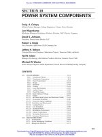
Voltages. Voltages of subtransmission circuits range from 12 to 345 kV, but today the levels of 69,
115, and 138 kV are most common. The use of the higher voltages is expanding rapidly as higher
FIGURE 18-6 Uniformly distributed loads.
Beaty_Sec18.qxd 17/7/06 8:53 PM Page 18-16
Downloaded from Digital Engineering Library @ McGraw-Hill (www.digitalengineeringlibrary.com)
Copyright © 2006 The McGraw-Hill Companies. All rights reserved.
Any use is subject to the Terms of Use as given at the website.
POWER DISTRIBUTION
POWER DISTRIBUTION 18-17
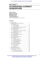
primary voltages are receiving increased usage.
Current practice as indicated by an informal util-
ity survey is shown in Fig. 18-7; 115 and 138 kV
together comprise about half the usage, 69 kV
about 20%; 230 kV usage is becoming substan-
tial, reflecting the growing use of 25- and 34.5-kV
primary distribution.
Conductors of ACSR or aluminum generally
have supplanted copper in overhead construc-
tion, and aluminum conductors are being used
increasingly in cables.
Voltage Regulation of Subtransmission. The
size of conductors used in subtransmission sys-
tems is determined by (1) magnitude and power factor of the load, (2) emergency loading require-
ments, (3) distance that the load must be carried, (4) operating voltage, (5) permissible voltage drop
under normal and emergency loading, and (6) optimal economic balance between installed cost of
the conductor and cost of losses. Table 18-2 gives the line-to-neutral voltage drops per 100,000 A и ft
for common cable and overhead conductor sizes and representative power factors for 34.5- and 69-kV
subtransmission. Values in the table are based on the approximate formula (18-4)

V
drop
ϭ IR cos ␪ ϩ IX sin ␪ ϭ IZ cos (␾ Ϫ ␪)
where R, X, and Z are 60-Hz resistance, reactance, and impedance in ohms per 1000 ft of a single con-
ductor, ␪ is the power-factor angle in electrical degrees, and ␾ is the impedance angle, tan
–1
(X/R).
Examples of How to Use Table 18-2. Determine the voltage drop when a 3-phase 20,000-kVA load
at 95% power factor is carried 10 mi over an overhead 69-kV circuit with No. 2/0 ACSR conductor.
Assuming the receiving-end voltage to be 69 kV, the current is
Circuit feet are
10 ϫ 5280 ϭ 52,800 ft
Thus
From the overhead portion of Table 18-2, the voltage drop per 100,000 A и ft at 95% power factor for
a No. 2/0 ACSR conductor is 19.1 V. Therefore, the total voltage drop for the example is 88.36 ϫ
19.1 ϭ 1687.68 V line-to-neutral. Since normal line-to-neutral voltage is ϭ 39.838 kV, or
39,838 V, the percent voltage drop is 1687.68 ϫ 100/39,838 ϭ 4.24%.
Assuming that permissible voltage drop is the limiting factor, what overhead ACSR conductor
size should be used to supply a load of 40,000 kVA at 95% power factor and receiving-end voltage
of 69 kV with a permissible drop of 5% and 8 mi between sending and receiving ends?

A
#
ft
100,000
ϭ
334.71 ϫ 42,240
100,000
ϭ 141.38
Circuit feet ϭ 8 ϫ 5280 ϭ 42,240 ft

Current ϭ
40,000
!3 ϫ 69
ϭ 334.71 A
69/!3

A
#
ft
100,000
ϭ
167.35 ϫ 52,800
100,000
ϭ 88.36
I ϭ
kVA
!3E
ϭ
20,000
!3 ϫ 69
ϭ 167.35 A
FIGURE 18-7 Use of distribution substation high-
voltage rating.
Beaty_Sec18.qxd 17/7/06 8:53 PM Page 18-17
Downloaded from Digital Engineering Library @ McGraw-Hill (www.digitalengineeringlibrary.com)
Copyright © 2006 The McGraw-Hill Companies. All rights reserved.
Any use is subject to the Terms of Use as given at the website.
POWER DISTRIBUTION
TABLE 18-2 Voltage Drops per 100,000 A ⋅ ft
*

for 3-Phase, 60-Hz, 34.5- and 69-kV Subtransmission
Voltage class
Approx. amp.
34.5 kV 69 kV
capacity for
Lagging power factor
air moving at
Conductor size 0.7 0.8 0.9 0.95 1.00 0.7 0.8 0.9 0.95 1.00 2 ft/s
Underground subtransmission
†
Aluminum:
No. 1/0 18.3 19.9 21.1 21.5 21.0
No. 2/0 15.4 16.5 17.4 17.6 16.9
No. 4/0 10.7 11.2 11.5 11.4 10.5
350 kcmil 7.69 7.84 7.77 7.55 6.50 8.04 8.10 7.92 7.62 6.38
500 kcmil 6.15 6.12 5.88 5.59 4.50 6.53 6.43 6.10 5.74 4.48
750 kcmil 4.96 4.80 4.44 4.10 3.00 5.25 5.05 4.63 4.23 3.01
1000 kcmil 4.32 4.12 3.73 3.37 2.30 4.69 4.44 3.96 3.55 2.32
Overhead subtransmission
‡
ACSR:
No. 4 42.9 45.5 47.3 47.5 44.7 43.6 46.1 47.7 47.8 44.7 120
No. 2 31.5 32.5 32.7 32.1 28.4 32.2 33.1 33.1 32.4 28.4 165
No. 1/0 24.1 24.1 23.2 22.1 18.0 24.8 24.7 23.7 22.4 18.0 225
No. 2/0 21.6 21.2 20.1 18.8 14.6 22.3 21.8 20.5 19.1 14.6 260
No. 4/0 17.3 16.6 15.1 13.8 9.66 18.0 17.2 15.5 14.1 9.66 355
336.4 kcmil 12.7 11.8 10.4 9.13 5.57 13.4 12.4 10.8
9.44 5.57 480
477 kcmil 11.2 10.3 8.72 7.44 3.92 12.0 10.9 9.15 7.75 3.92 605
795 kcmil 9.73 8.68 7.06 5.78 2.37 10.4 9.28 7.49 6.09 2.37 850

Note: 1 in ϭ 25.4 mm; 1 in
2
ϭ 645 mm
2
; 1 ft ϭ 0.3048 m. Regulation of copper conductors can be estimated with reasonable accurac
y as that of aluminum conductors two sizes larger. For ampac-
ities of cables, see Tables 18–22 and 18–23.
*
Values in the table give the difference in absolute value between sending-end and recei
ving-end line-to-neutral voltages of a balanced 3-phase circuit.
†
Underground cable impedances are based on 90ЊC conductor temperature with close triangular spacing of cables using typical solid-dielectric insulation, 100% insulation le
vel, single conductor,
shielded and jacketed.
‡
Overhead conductor impedances are based on 50ЊC conductor temperature, ACSR construction, 600 A/in
2
density with 60-in equivalent spacing for 35 kV and 90 in for 69 kV
.
18-18
Beaty_Sec18.qxd 17/7/06 8:53 PM Page 18-18
Downloaded from Digital Engineering Library @ McGraw-Hill (www.digitalengineeringlibrary.com)
Copyright © 2006 The McGraw-Hill Companies. All rights reserved.
Any use is subject to the Terms of Use as given at the website.
POWER DISTRIBUTION
POWER DISTRIBUTION 18-19
The permissible voltage drop is V line-to-neutral. The corre-
sponding permissible voltage drop per 100,000 A и ft is
From Table 18-2 it is seen that this corresponds approximately to No. 4/0 ACSR.
Subtransmission System Patterns. A wide variety of subtransmission system designs are in use,

varying from simple radial systems to systems similar to networks. The radial system is not generally
used because most utilities today plan their subtransmission-
distribution substation systems so that one major contin-
gency such as outage of a subtransmission circuit or failure
of a distribution substation transformer will not result in loss
of load—or at least the loss of load will be of short duration
while automatic switching operations take place. Thus, loop
and multiple circuit patterns predominate. Figures 18-8 and
18-9 illustrate the basic nature of these two patterns. The
loop pattern implies that a single circuit originating at one
bulk power source “loops” through several substations
before terminating at another bulk source or even at the orig-
inal source. Reinforcing ties, as indicated by the dotted con-
nection, are used when the number of substations exceeds
some predetermined level.
Multiple circuit pattern implies the use of two or more
circuits which are tapped at each substation, as illustrated in
Fig. 18-9. The circuits may be radial or may terminate in a second bulk power source. Many varia-
tions of the two basic patterns are found. From a recent informal survey of approximately 50 major
utilities, it appears that the two patterns are about equally used.
1991.92
141.38
ϭ 14.1 V/100,000 A
#
ft
0.05 ϫ 69,000/!3
ϭ 1991.92
FIGURE 18-8 Loop pattern.
FIGURE 18-9 Multiple pattern.
Beaty_Sec18.qxd 17/7/06 8:53 PM Page 18-19

Downloaded from Digital Engineering Library @ McGraw-Hill (www.digitalengineeringlibrary.com)
Copyright © 2006 The McGraw-Hill Companies. All rights reserved.
Any use is subject to the Terms of Use as given at the website.
POWER DISTRIBUTION
18-20 SECTION EIGHTEEN
A vast majority of today’s subtransmission is of overhead construction, much of it built on city
streets as contrasted with private rights of way. However, appearance and environmental considera-
tions, difficulty in obtaining substation sites and rights of way, and rapid growth of underground dis-
tribution are certain to exert continuing pressure on the undergrounding of subtransmission. Even
with the use of direct-buried, solid-dielectric cables, the cost of underground subtransmission is
many times the cost of overhead circuits, particularly where the overhead subtransmission can be
built on city streets.
Thus, a requirement to build future subtransmission underground would have major impact on the
balance of overall subtransmission-substation-primary distribution costs. It undoubtedly would focus
attention on minimizing the amount of subtransmission circuitry needed to cover the load area,
which in turn would favor
Fewer, larger substations
Loop subtransmission pattern rather than multiple parallel circuits
Depending on load density in this area, it could favor
Higher primary voltage
Higher subtransmission voltage
Changes in either subtransmission or primary voltage levels are major decisions which require study
in depth and ultimately the commitment of large financial resources.
18.6 PRIMARY DISTRIBUTION SYSTEMS
The primary distribution system takes energy from the low-voltage bus of distribution substations
and delivers it to the primary windings of distribution transformers.
Overhead Primary Systems. Typically, overhead primary distribution systems have been operated
as radial circuits (normally open loops) from the substation outward. Figure 18-2 shows schemati-
cally a typical primary feeder in a predominantly residential area; an overhead 12.47Y/7.2-kV sys-
tem is used for illustrative and functional purposes, but underground systems will be discussed later.

The main feeder backbone usually is a 3-phase 4-wire circuit from which the single-phase lateral
or branch circuits are tapped through fuse cutouts to protect the system from faults on the lateral cir-
cuits. The single-phase lateral circuits consist of one phase conductor and the neutral. Distribution
transformers are connected between the phase and the neutral; in this case they would have a rating
of 7200 V.
Utilities use automatic reclosing feeder breakers and line reclosers to minimize service interrup-
tions. However, serious problems involving the main will cause an outage to some or all of the feeder
until line crews can locate the problem and manually operate pole-top disconnecting switches appro-
priately to isolate the problem and to pick up as much load as possible from adjacent feeders.
Switches of this kind usually are found in both the main and lateral circuits, as indicated in Fig. 18-2.
Also, it is often possible to make and to remove connections while the system is energized through
the use of hot-line tools, hot-line clamps, insulated bucket trucks, etc.
Generally, this approach has provided an acceptable level of service because overhead system
troubles are relatively easy to locate, and repair times are short. However, when the entire primary
system is installed underground, while the frequency of serious trouble is expected to be lower than
in overhead systems, it is likely that the time involved in pinpointing the location and making repairs
will be much longer than in overhead systems.
Underground System. While a relatively small percentage of new general-purpose feeders is
being installed totally underground, the trend is growing and is expected to continue to grow.
Beaty_Sec18.qxd 17/7/06 8:53 PM Page 18-20
Downloaded from Digital Engineering Library @ McGraw-Hill (www.digitalengineeringlibrary.com)
Copyright © 2006 The McGraw-Hill Companies. All rights reserved.
Any use is subject to the Terms of Use as given at the website.
POWER DISTRIBUTION
POWER DISTRIBUTION 18-21
Since it is difficult to accomplish many maintenance and operating functions on an underground
system while it is “hot,” or energized, in contrast to overhead-system practices, specific provisions
must be made in the system design to incorporate needed sectionalizing and overcurrent protec-
tive equipment.
The main feeder plan shown in Fig. 18-10 is reasonably typical of present practice on under-

ground systems supplying basically residential and small commercial loads. Note that the main feed-
ers are operated radially, but with normally open ties to adjacent main feeders. The main feeder
switches usually are 3-phase, 600-A, manually operated load-break switches. The single-phase and
3-phase lateral circuits also are operated as normally open loops.
Switching in the 200-A circuits can be accomplished by means of either load-break switches or
separable, insulated cable connectors. Usually, two main feeder switches are grouped along with the
lateral circuit switching and protective equipment into one piece of pad-mounted equipment.
The primary feeders supplying secondary-network systems in metropolitan areas usually are
radial 3-wire circuits consisting of 3/c cables in underground duct lines. The 3-phase network trans-
formers are T-tapped to the primary feeders.
Automation. With increasing emphasis on reliability of service, a definite trend is under way to
make greater use of protective and sectionalizing equipment in the primary system in order to min-
imize the number of customers involved in an outage and to reduce the outage time. Proposed
schemes run the gamut from manually operated devices to automatic devices remotely controlled
from distribution centers. The remote-controlled schemes vary from some type of supervisory con-
trol to computer-controlled systems with built-in logic to cope quickly with the various problems
which may arise.
Primary-Distribution-System Voltage Levels. Since World War II, the 15-kV distribution class has
become firmly entrenched and today represents 60% to 80% of all primary distribution activity. Very
little expansion of lower-voltage systems is taking place. There is a trend, however, toward increas-
ing usage of primary voltage levels above the 15-kV class. This trend has an impact on substation
and subtransmission practices as well because higher primary voltages almost axiomatically lead to
larger substations and higher subtransmission voltages.
FIGURE 18-10 Typical main-feeder underground circuit. (All switches closed unless shown
otherwise.)
Beaty_Sec18.qxd 17/7/06 8:53 PM Page 18-21
Downloaded from Digital Engineering Library @ McGraw-Hill (www.digitalengineeringlibrary.com)
Copyright © 2006 The McGraw-Hill Companies. All rights reserved.
Any use is subject to the Terms of Use as given at the website.
POWER DISTRIBUTION

18-22 SECTION EIGHTEEN
The two principal voltages above 15 kV are 24.49Y/14.4 kV and 34.5Y/19.92 kV. New line addi-
tions at these voltage levels now average more than 20% of those at 15 kV.
To achieve economy, the higher primary voltages also require heavier feeder loadings which
could imply reduced service reliability because more customers are affected by primary faults.
Greater use of automatic switching and protective equipment can do much toward preserving
a level of reliability to which the public has become accustomed. This is another reason that
most observers believe that an increased amount of automation is inevitable in our distribution
systems.
For example, a typical 12.47-kV feeder serves a normal peak load on the order of 6000 to 7000 kVA.
On this basis, the probable peak loading of a fully developed 34.5-kV feeder would be expected to
be in the neighborhood of 18,000 to 20,000 kVA.
Why go to high-voltage distribution (HVD)? Most of today’s systems in the 15-kV class are not
voltage-drop-limited, and cost of higher-voltage laterals and associated equipment needed to cover
the load area is greater. The major economic advantages are:
1. Larger (and fewer) substations
2. Fewer circuits
3. Possibility of eliminating a system voltage-transformation level where the new primary voltage is
the former subtransmission level
Other advantages of HVD which are difficult to evaluate in dollars are:
1. Reduced losses in early stages of development
2. Reduced voltage regulation
3. Greater distance or area coverage
4. Fewer circuits per route (reduced congestion)
5. Fewer circuit positions at substations
6. Fewer substation sites
7. Greater flexibility in supplying large spot loads
Some of the disadvantages of HVD have been
1. Cost of equipment
2. Reliability due to increased exposure

3. Higher equipment failure rates
4. Operability
Conductor Sizes. The conductor sizes used in overhead primaries generally range from No. 2
AWG to 795 kcmil. ACSR and aluminum conductors have almost entirely displaced copper for new
construction. Aerial cable is used occasionally for primary conductors in special situations where
clearances are too close for open-wire construction or where adequate tree trimming is not
practical. The type of construction more frequently used consists of covered conductors (nonshielded)
supported from the messenger by insulating spacers of plastic or ceramic material. The conductor
insulation, usually a solid dielectric such as polyethylene, has a thickness of about 150 mils for a 15-kV
class circuit and is capable of supporting momentary contacts with tree branches, birds, and animals
without puncturing. This type of construction is commonly referred to as spacer cable.
The conductor sizes most commonly used in underground primary distribution vary from
No. 4 AWG to 1000 kcmil. Four-wire main feeders may employ 3- or 4-conductor cables, but single-
conductor concentric-neutral cables are more popular for this purpose. The latter usually employ
crosslinked polyethylene insulation, and often have a concentric neutral of one-half or one-third of
the main conductor cross-sectional area.
Beaty_Sec18.qxd 17/7/06 8:53 PM Page 18-22
Downloaded from Digital Engineering Library @ McGraw-Hill (www.digitalengineeringlibrary.com)
Copyright © 2006 The McGraw-Hill Companies. All rights reserved.
Any use is subject to the Terms of Use as given at the website.
POWER DISTRIBUTION
POWER DISTRIBUTION 18-23
The smaller-sized cables used in lateral circuits of URD systems are nearly always single-conductor,
concentric-neutral, crosslinked polyethylene-insulated, and usually directly buried in the earth.
Insulation thickness is on the order of 175 mils for 15-kV-class cables and 345 mils for 35-kV class
with 100% insulation level.
Stranded or solid aluminum conductors have virtually supplanted copper for new construction,
except where existing duct sizes are restrictive. With the solid-dielectric construction, in order to
limit voltage gradient at the surface of the conductor within acceptable limits, a minimum conductor
size of No. 2 AWG is common for 15-kV-class cables, and No. 1/0 AWG for 35-kV class.

Voltage Regulation of Primary Distribution. Table 18-3 can be used to determine the voltage drop
of an existing circuit when the load data are known or to determine minimum conductor size required
to meet a given voltage-drop limit. Data are given for various underground-cable and overhead-
conductor configurations for 12.47 and 34.5 kV.
Example. What is the voltage drop for a 34.5-kV overhead circuit 3 mi long using 4/0 alu-
minum conductor and carrying a balanced 3-phase load of 15,000 kVA at 90% power factor: The cur-
rent is 15,000/ ϫ 34.5 ϭ 251 A. The circuit feet are 3 ϫ 5280 ϭ 15,840 ft. Thus A ⋅ ft/100,000 ϭ
251 ϫ 15,840/100,000 ϭ 39.758. From Table 18-3, the appropriate voltage drop per 100,000 A и ft
is 14.0 V line-to-neutral. Therefore, the total voltage drop for the example is
39.758 ϫ 14.0 ϭ 556.6 V line-to-neutral
Since normal line-to-neutral voltage is 34,500 ϭ 19,920 V, the percent voltage drop is
556.6 ϫ 100/19,920 ϭ 2.79%
Example. What is the minimum aluminum conductor size to carry 6000 kVA at 90% power factor
of balanced 3-phase load over a 2-mi, 12.47Y/7.2-kV feeder with no more than a 3% voltage drop?
Load current is 6000/ ϫ 12.47 ϭ 277.8 A. Circuit feet ϭ 2 ϫ 5280 ϭ 10,560 ft. Thus
The corresponding drop per 100,000 A и ft is 216/29.34 ϭ 7.36 V, line-to-neutral. From Table 18-3,
this value falls between 477 and 795 kcmil, so that the latter size would be chosen.
Loading. Loading of primary feeders varies greatly depending on primary voltage, load density,
emergency loading requirements, etc. Typical peak loads on 15-kV class feeders are 6 to 7000 kVA.
Peak loads on 25- and 35-kV class, fully developed feeders probably will be proportionally greater
in the future, assuming that appropriate measures can be taken to maintain acceptable reliability of
service.
Voltage Drop. Voltage drop in the primary feeder is an important factor in system design; however,
it is only one of the many voltage-drop considerations involved in determining the range of voltages
delivered to the customers’ service entrances. American National Standard, “Voltage Ratings for
Electric Power Systems and Equipment (60-Hz),” ANSI C84.1-1995 (R200), defines in detail the
voltage ranges which should be observed. Outside the distribution substation, voltage drops occur in
the primary system, the distribution transformer, the secondary system, the service drop, and in the
users’ wiring systems as well. Remedial measures, such as voltage regulators and shunt capacitor
banks, can be used to counteract or reduce the voltage drop due to load flow.

A traditional rough rule of thumb has been to allow a voltage drop of about 3% in the primary of
urban and suburban systems at time of peak load. Actually, with typical load densities and primary
systems of 15-kV class or higher, it is very probable that economic system designs have a primary
voltage drop smaller than 3%.
Permissible voltage drop ϭ 0.03 ϫ
12,470
23
ϭ 216 V

A
#
ft
100,000
ϭ
277.8 ϫ 10,560
100,000
ϭ 29.34
!3
!3
!3
Beaty_Sec18.qxd 17/7/06 8:53 PM Page 18-23
Downloaded from Digital Engineering Library @ McGraw-Hill (www.digitalengineeringlibrary.com)
Copyright © 2006 The McGraw-Hill Companies. All rights reserved.
Any use is subject to the Terms of Use as given at the website.
POWER DISTRIBUTION
TABLE 18-3 Line-to-Neutral Voltage Drops per 100,000 A ⋅ ft
*
for 12.47Y/7.2 and 34.5Y/19.92 kV and Balanced 3-Phase Loads
Voltage class
12.47Y/7.2 kV

34.5Y/19.92 kV
Lagging power factor
Conductor size 0.7 0.8 0.9 0.95 1.00 0.7 0.8 0.9 0.95 1.00
Underground primary
Aluminum:
Concentric neutral—direct buried, cross-linked polyethylene, conductor 70
ЊC, neutral 60ЊC, earth resistivity 90 ⍀ ⋅ cm
3
, triplex configuration, full installation
No. 1/0 17.1 18.5 19.8 20.2 19.8 17.6 19.0 20.1 20.4 19.8
No. 2/0 14.1 15.1 16.0 16.3 15.7 14.6 15.6 16.3 16.5 15.7
No. 4/0 9.82 10.4 10.7 10.7 9.96 10.3 10.8 11.0 10.9 9.95
350 kcmil 7.01 7.19 7.17 7.00 6.11 7.37 7.49 7.39 7.16 6.11
500 kcmil 5.66 5.69 5.55 5.31 4.40 6.04 6.00 5.76 5.47 4.40
750 kcmil 4.63 4.55 4.30 4.03 3.12 4.95 4.82 4.49 4.16 3.11
1000 kcmil 4.10 3.98 3.69 3.41 2.52 4.37 4.20 3.85 3.52 2.51
Single conductor shielded and jacked, cross-lined polyethylene, conductor 70
ЊC, unigrounded shield, triplex configuration, full insulation
350 kcmil 7.29 7.49 7.51 7.35 6.47 7.55 7.72 7.67 7.47 6.47
500 kcmil 5.78 5.82 5.67 5.45 4.54 6.08 6.07 5.86 5.58 4.54
750 kcmil 4.64 4.54 4.26 3.97 3.02 4.88 4.74 4.41 4.08 3.02
1000 kcmil 4.02 3.85 3.52 3.21 2.26 4.23 4.03 3.65 3.31 2.26
Overhead primary
†
No. 4 42.3 45.4 47.8 48.5 46.6 43.4 46.3 48.5 49.0 46.6 115
No. 2 29.8 31.2 32.0 31.9 29.3 30.9 32.2 32.7 32.4 29.3 160
No. 1/0 21.8 22.2 22.1 21.5 18.5 23.0 23.2 22.8 22.0 18.5 215
No. 2/0 19.0 19.1 18.6 17.8 14.7 20.1 20.0 19.3 18.3 14.7 250
No. 4/0 14.7 14.3 13.3 12.4 9.20 15.9 15.3 14.0 12.7 9.20 340
336.4 kcmil 11.8 11.2 9.97 8.91 5.80 13.0 12.1 10.7

9.41 5.80 465
477 kcmil 10.4 9.58 8.27 7.18 4.10 11.5 10.5 8.97 7.68 4.10 590
795 kcmil 8.22 7.92 6.52 5.40 2.40 9.96 8.88 7.22 5.90 2.40 820
Note: 1 in ϭ 25.4 mm; 1 ft ϭ 0.3048 m. For ampacities of cables, see Tables 18-23 and 18-24. Re
gulation of copper for overhead conductors can be estimated with reasonable accuracy the same
as that of aluminum conductors two sizes larger. For single-phase o
verhead primaries, the voltage drop is approximately two times the 3-phase values given in the table. For underground single-phase
primaries in concentric-neutral, direct-buried cables, see section on URD systems. Cables are 15- and 35-kV classes, respecti
vely.
*
Values in the table give the difference in absolute value between sending-end and recei
ving-end line-to-neutral voltages of a balanced 3-phase circuit, in v
olts.
†
Overhead conductor impedances are based on 50ЊC conductor temperature, aluminum conductor with 30-in equi
valent spacing for 12.47Y kV and 60-in for 34.5Y kV.
Approx. amp.
capacity for
air moving at
2 ft/s
18-24
Beaty_Sec18.qxd 17/7/06 8:53 PM Page 18-24
Downloaded from Digital Engineering Library @ McGraw-Hill (www.digitalengineeringlibrary.com)
Copyright © 2006 The McGraw-Hill Companies. All rights reserved.
Any use is subject to the Terms of Use as given at the website.
POWER DISTRIBUTION
POWER DISTRIBUTION 18-25
In rural systems which are typified by long lines and light load densities, primary voltage drops
may be somewhat larger. This is offset somewhat by the absence of secondaries in serving individ-
ual farms; however, the service drops often are longer than in urban systems. The design objective,

of course, is to keep delivered voltage to all customers in an acceptable and satisfactory range.
18.7 THE COMMON-NEUTRAL SYSTEM
The 4-wire, multigrounded, common-neutral distribution system now is used almost exclusively
because of the economic and operating advantages it offers. Usually, the windings of the substation
transformers serving the primary system are wye-connected, and the neutral point is solidly
grounded. Occasionally, a small amount of impedance is connected between the transformer neutral
and ground in order to limit line-to-ground short-circuit currents on the primary system to a prede-
termined value. The neutral circuit must be a continuous metallic path along the primary routes of
the feeder and to every user location. Where primary and secondary systems are both present, the
same conductor is used as the “common” neutral for both systems. The neutral is grounded at each
distribution transformer, at frequent intervals where no transformers are connected, and to metallic
water pipes or driven grounds at each user’s service entrance. The neutral carries a portion of the
unbalanced or residual load currents for both the primary and secondary systems. The remainder of
this current flows in the earth and/or the water system. For typical conditions, it is estimated that
about one-half the return current flows in the neutral conductor, although the division can vary
widely depending on earth resistivity and the relative routing of the electric and water systems.
Figure 18-11 is a schematic representation of a common-neutral system.
Grounding of Neutral. Rules related to grounding on the utility system neutral are given in the
National Electrical Safety Code (NESC), ANSI C2, and regulations governing the grounding of
the neutral on users’ premises are stated in the National Electrical Code (NEC), NFPA 70. In brief,
the secondary neutral is grounded at every service through a metallic water-piping system and
through “made electrode grounds” such as other underground metal systems, building steel, or dri-
ven ground electrodes. The increasing use of nonmetallic water piping and insulating couplings on
metal water systems is requiring the use of other grounding means. The secondary neutral also is
grounded at the distribution transformer, usually by means of driven grounds. Although it is often
FIGURE 18-11 Common-neutral methods of distribution.
Beaty_Sec18.qxd 17/7/06 8:53 PM Page 18-25
Downloaded from Digital Engineering Library @ McGraw-Hill (www.digitalengineeringlibrary.com)
Copyright © 2006 The McGraw-Hill Companies. All rights reserved.
Any use is subject to the Terms of Use as given at the website.

POWER DISTRIBUTION