fischer-cripps, a. c. (2002). newnes interfacing companion
Bạn đang xem bản rút gọn của tài liệu. Xem và tải ngay bản đầy đủ của tài liệu tại đây (4.1 MB, 308 trang )
Newnes Interfacing Companion
To Robert Winston Cheary,
friend and teacher.
OXFORD AMSTERDAM BOSTON LONDON NEW YORK PARIS
SAN DIEGO SAN FRANCISCO SINGAPORE SYDNEY TOKYO
Newnes
An imprint of Elsevier Science
Linacre House, Jordan Hill, Oxford OX2 8DP
225 Wildwood Avenue, Woburn MA 01801-2041
First published 2002
Copyright 2002, A. C. Fischer-Cripps. All rights reserved
The right of A. C. Fischer-Cripps to be identified as the author of this work
has been asserted in accordance with the Copyright, Designs and
Patents Act 1988
No part of this publication may be reproduced in any material form (including
photocopying or storing in any medium by electronic means and whether
or not transiently or incidentally to some other use of this publication) without
the written permission of the copyright holder except in accordance with the
provisions of the Copyright, Designs and Patents Act 1988 or under the terms of
a licence issued by the Copyright Licensing Agency Ltd, 90 Tottenham Court Road,
London, England W1T 4LP. Applications for the copyright holder's written
permission to reproduce any part of this publication should be addressed
to the publisher
British Library Cataloguing in Publication Data
A catalogue record for this book is available from the British Library
Library of Congress Cataloguing in Publication Data
A catalogue record for this book is available from the Library of Congress
ISBN 0 750 65720 0
For information on all Newnes publications
visit our website at www.newnespress.com
Printed and bound in Great Britain
Preface ix
Part 1: Transducers 1
1.0 Transducers 2
1.1 Measurement systems 3
1.1.1 Transducers 4
1.1.2 Methods of measurement 5
1.1.3 Sensitivity 6
1.1.4 Zero, linearity and span 7
1.1.5 Resolution, hysteresis and error 8
1.1.6 Fourier analysis 9
1.1.7 Dynamic response 10
1.1.8 PID control 11
1.1.9 Accuracy and repeatability 12
1.1.10 Mechanical models 13
1.1.11 Review questions 14
1.2 Temperature 15
1.2.1 Temperature 16
1.2.2 Standard thermometers 17
1.2.3 Industrial thermometers 18
1.2.4 Platinum resistance thermometer 19
1.2.5 Liquid-in-glass thermometer 20
1.2.6 Radiation pyrometer 21
1.2.7 Thermocouple 22
1.2.8 Thermistors 24
1.2.9 Relative humidity 25
1.2.10 Review questions 26
1.2.11 Activities 28
1.3 Light 34
1.3.1 Light 35
1.3.2 Measuring light 36
1.3.3 Standards of measurement 37
1.3.4 Thermal detectors 38
1.3.5 Light dependent resistor (LDR) 39
1.3.6 Photodiode 40
1.3.7 Other semiconductor photodetectors 41
1.3.8 Optical detectors 42
1.3.9 Photomultiplier 43
1.3.10 Review questions 44
1.4 Position and motion 45
1.4.1 Mechanical switch 46
1.4.2 Potentiometric sensor 47
1.4.3 Capacitive transducer 48
1.4.4 LVDT 49
1.4.5 Angular velocity transducer 50
1.4.6 Position sensitive diode array 51
1.4.7 Motion control 52
1.4.9 Review questions 53
1.5 Force, pressure and flow 54
1.5.1 Strain gauge 55
1.5.2 Force 57
1.5.3 Piezoelectric sensor instrumentation 58
1.5.4 Acceleration and vibration 59
1.5.5 Mass 60
1.5.6 Atmospheric pressure 61
1.5.7 Pressure 63
1.5.8 Industrial pressure measurement 64
1.5.9 Sound 65
1.5.10 Flow 66
1.5.11 Level 69
1.5.12 Review questions 70
Part 2: Interfacing 71
2.0 Interfacing 72
2.1 Number systems 73
2.1.1 Binary number system 74
2.1.2 Decimal to binary conversion 75
2.1.3 Hexadecimal 76
2.1.4 Decimal to hex conversion 77
2.1.5 2s complement 78
2.1.6 Signed numbers 79
2.1.7 Subtraction and multiplication 80
2.1.8 Binary coded decimal (BCD) 81
2.1.9 Gray code 82
2.1.10 ASCII code 83
2.1.11 Boolean algebra 84
2.1.12 Digital logic circuits 85
2.1.13 Review questions 86
2.1.14 Activities 87
2.2 Computer architecture 88
2.2.1 Computer architecture 89
2.2.2 Memory 90
2.2.3 Segmented memory 91
2.2.4 Memory data 92
2.2.5 Buffers 93
2.2.6 Latches 94
2.2.7 Flip-flop 95
2.2.8 Input/Output (I/O) 96
2.2.9 Microprocessor unit (MPU/CPU) 97
2.2.10 Registers 98
2.2.11 ROM 101
2.2.12 Interrupts 102
2.2.13 Memory map 104
2.2.14 Real and protected mode CPU
operation 105
2.2.15 Review questions 107
2.2.16 Activities 108
2.3 Assembly language 111
2.3.1 Instruction set 112
2.3.2 Assembly language 113
2.3.3 Program execution 114
2.3.4 Assembly language program structure 115
2.3.5 Assembler directives 116
2.3.6 Code segment 117
2.3.7 Assembly language shell program 118
2.3.8 Branching 119
2.3.9 Register and immediate addressing 120
2.3.10 Memory addressing 121
2.3.11 Indirect memory addressing 122
2.3.12 Indexed memory addressing 123
2.3.14 Interrupts 124
2.3.15 Review questions 125
2.3.16 Activities 126
2.4 Interfacing 131
2.4.1 Interfacing 132
2.4.2 Input/Output ports 133
2.4.3 Polling 134
2.4.4 Interrupts 135
2.4.5 Direct memory access (DMA) 136
2.4.6 Serial port 137
2.4.7 Serial port addresses 138
2.4.8 Serial port registers 139
2.4.9 Serial port registers and interrupts 140
2.4.10 Serial port baud rate 141
2.4.11 Serial port operation 142
2.4.12 Parallel printer port 143
2.4.13 Parallel port registers 144
2.4.14 Parallel printer port operation 145
2.4.15 Review questions 146
2.5 A to D and D to A conversions 147
2.5.1 Interfacing 148
2.5.2 The Nyquist criterion 149
2.5.3 Resolution and quantisation noise 150
2.5.4 Oversampling 151
2.5.5 Analog to digital converters 152
2.5.6 ADC (integrating method) 153
2.5.7 ADC (successive approximation) 154
2.5.8 Aperture error 155
2.5.9 ADC08xx chip 156
2.5.10 Sample-and-hold 157
2.5.11 Sample-and-hold control 158
2.5.12 Digital to analog conversion 159
2.5.13 DAC0800 160
2.5.14 Data acquisition board 161
2.5.15 Review questions 162
2.6 Data communications 163
2.6.1 Communications 164
2.6.2 Byte to serial conversion 165
2.6.3 RS232 interface 166
2.6.4 Synchronisation 167
2.6.5 UART (6402) 168
2.6.7 Line drivers 170
2.6.8 UART clock 171
2.6.9 UART Master Reset 172
2.6.10 Null modem 173
2.6.11 Serial port BIOS services 174
2.6.12 Serial port operation in BASIC 175
2.6.13 Hardware handshaking 176
2.6.14 RS485 177
2.6.15 GPIB 178
2.6.16 USB 179
2.6.17 TCP/IP 181
2.6.18 Review questions 182
2.7 Programmable logic controllers 183
2.7.1 Programmable logic controllers 184
2.7.2 Timing 185
2.7.3 Functional components 186
2.7.4 Programming 187
2.7.5 Ladder logic diagrams 188
2.7.6 PLC specifications 190
2.7.7 Review questions 191
2.8 Data acquisition project 192
2.8.1 Serial data acquisition system 193
2.8.2 Circuit construction 195
2.8.3 Programming 201
2.8.4 Sample-and-hold 206
2.8.5 Digital to analog system 208
Part 3: Signal processing 211
3.0 Signal processing 212
3.1 Transfer function 213
3.1.1 Instrumentation 214
3.1.2 Transfer function 215
3.1.3 Transforms 216
3.1.4 Laplace transform 217
3.1.5 Operator notation 218
3.1.6 Differential operator 219
3.1.7 Integrator passive 220
3.1.8 Differentiator passive 221
3.1.9 Transfer impedance 222
3.1.10 Review questions 223
3.1.11 Activities 224
3.2 Active filters 227
3.2.1 Filters 228
3.2.2 T -network filters 229
3.2.3 Twin-T filter 230
3.2.4 Active integrator/differentiator 231
3.2.5 Integrator transfer function 232
3.2.6 Low pass filter active 233
3.2.7 2nd order active filter 234
3.2.8 Double integrator 235
3.2.9 Bandpass filter narrow 236
3.2.10 Differentiator transfer function 237
3.2.11 High pass filter active 238
3.2.12 High pass filter w domain 239
3.2.13 Bandpass filter wide 240
3.2.14 Voltage gain and dB 241
3.2.15 Review questions 242
3.2.16 Activities 244
3.3 Instrumentation amplifier 246
3.3.1 Difference amplifier 247
3.3.2 CMRR 248
3.3.3 Difference amplifier with voltage
follower inputs 249
3.3.4 Difference amplifier with cross-coupled
inputs 250
3.3.5 CMRR cross-coupled inputs 251
3.3.6 Instrumentation amplifier 252
3.3.7 Log amplifier 253
3.3.8 Op-amp frequency response 254
3.3.9 Review questions 255
3.3.10 Activities 257
3.4 Noise 261
3.4.1 Intrinsic noise 262
3.4.2 Environmental noise 263
3.4.3 Signal-to-noise ratio 264
3.4.4 Optical detectors 265
3.4.5 Lock-in amplifier 266
3.4.6 Correlation 267
3.4.7 Review questions 268
3.5 Digital signal processing 269
3.5.1 Digital filters 270
3.5.2 Fourier series 271
3.5.3 Fourier transform 272
3.5.4 Sampling 273
3.5.5 Discrete Fourier transform 274
3.5.6 Filtering 275
3.5.7 Digital filtering (domain) 276
3.5.8 Convolution 277
3.5.9 Discrete convolution 278
3.5.10 Digital filtering (t-domain) 279
3.5.11 Example 280
3.5.12 Smoothing transfer function 281
3.5.13 Review questions 282
3.5.14 Activities 283
Index 286
Further reading 294
Parts lists for activities 295
Preface
The overall aim of this book is to present transducer devices,
computer interfacing and instrumentation electronics in a succinct
and memorable fashion. The book combines physics, computer
science and electrical engineering in a science/engineering context.
Starting from the transfer of physical phenomena to electrical signals,
the book presents a comprehensive treatment of computer interfacing
and finishes with signal conditioning, data analysis and digital
filtering. The book covers a wide scope but contains sufficient detail
to allow a practical application of the theory. Detailed explanations
are given, even of the most difficult of concepts. The review
problems offer a level of complexity which provides sufficient
challenge to impart a sense of achievement upon their completion.
The accompanying project work reinforces the theoretical work
while allowing the reader to gain the satisfaction and experience of
actually constructing a working interfacing circuit that can be used
on any personal computer with a serial port. The book will be useful
for students who are new to the subject, and will serve as a handy
reference for experienced engineers who wish to refresh their
knowledge of a particular topic.
In writing this book, I was assisted and encouraged by many
colleagues. In particular, I acknowledge the contributions of Alec
Bendeli, Stephen Buck, Bob Graves, Walter Kalceff, Les Kirkup,
Geoff Smith, Paul Walker, my colleagues at the University of
Technology, Sydney, the staff of the CSIRO Division of
Telecommunications and Industrial Physics, and all my former
students. My sincere thanks to my wife and family for their unending
encouragement and support. Finally, I thank Matthew Deans, Jodi
Burton and the editorial and production teams at Newnes for their
very professional and helpful approach to the whole publication
process.
Tony Fischer-Cripps,
Killarney Heights, Australia, 2002
ix
Newnes Interfacing Companionx
1
1.0 Transducers
A measurement system is concerned with the representation of one
physical phenomenon by another. The purpose of the measurement system
is for the measurement and control of a physical system.
In Part 1 of this book,
we are mainly interested
in transducers.
•A sensor is a device
which responds to a
physical stimulus
•A transducer is a
device which converts a
physical stimulus to
another form of energy
(usually electrical)
Physical
phenomena:
Sound
Meter reading
LED indicator
Digital display
Chart recorder
VDU output
Physical
phenomena:
Temperature
Voltage
Position
Velocity
Force
Pressure
Radioactivity
Light intensity
Resistance
Humidity
Gas concentration
Magnetic field
Frequency
Sound level
Actuator
provides a
physical
response to
electrical signal.
Actuator
Optional
feedback
Transducer
(sensor and
preamplifier)
Amplifier and
signal
conditioning
Computer
interface
Part 2 of this
book is
concerned with
computer
interfacing.
Part 3 of this
book covers
instrumentation
and signal
processing.
Newnes Interfacing Companion2
3
1.1.1 Transducers
Of most interest are the physical properties and performance
characteristics of a transducer. Some examples are given below:
Strain Strain gauge, a resistive transducer whose resistance
changes with length.
Temperature Resistance thermometer, thermocouple, thermister,
thermopile.
Humidity Resistance change of hygroscopic material.
Pressure Movement of the end of a coiled tube under
pressure.
Voltage Moving coil in a magnetic field.
Radioactivity Electrical pulses resulting from ionisation of gas at
low pressure.
Magnetic field Deflection of a current carrying wire.
Property Method of measurement
Performance characteristics
Sensitivity
Zero offset
Linearity
Range
Span
Resolution
Threshold
Hysteresis
Repeatability
Response time
Damping
Natural frequency
Frequency response
Operating temperature
range
Orientation
Vibration/shock
Static Dynamic Environmental
A consideration of these characteristics influences the
choice of transducer for a particular application.
Further characteristics which are often important are
the operating life, storage life, power requirements
and safety aspects of the device as well as cost and
availability of service.
In industrial situations, the property being measured or controlled is called
the controlled variable. Process control is the procedure used to measure
the controlled variable and control it to within a tolerance level of a set
point. The controlled variable is one of several process variables and is
measured using a transducer and controlled using an actuator.
Newnes Interfacing Companion4
An unknown component is inserted into the
bridge and the values of the others are
altered to achieve balance condition.
At balance, no
current flows
through the
galvanometer G.
Null method
Deflection method
• Direct comparison
• No loading
• Can be relatively slow
• Indirect comparison
• Deflection from zero until
some balance condition
achieved
• Limited in precision and
accuracy
• Loading (transducer itself
takes some energy from
the system being
measured)
• Relatively fast
Null method: Bridge circuit.
3
u
4
1
3
u
41
C
R
C
R
C
L
RR
=
=
Deflection method:
Moving coil voltmeter.
1.1.2 Methods of measurement
All measurements involve a
comparison between a
measured quantity and a
reference standard. There
are two fundamental
methods of measurement:
Although such a meter is designed to have a
very high internal impedance, it has to draw
some current from the circuit being measured
in order to cause a deflection of the pointer.
This may affect the operation of the circuit
itself and lead to inaccurate readings –
especially if the output resistance of the
voltage source being measured is large.
pointer
coil
magnet
C
3
R
1
C
4
R
u
L
u
R
4
G
1.1 Measurement systems 5
1.1.3 Sensitivity
An important parameter associated with every transducer is its sensitivity.
This is a measure of the magnitude of the output divided by the magnitude
of the input.
dI
dO
signalinput
signaloutput
ysensitivit
=
=
In most applications, the chances are that the signal produced by the
transducer contains noise, or unwanted information. The proportion of
wanted to unwanted signal is called the signal-to-noise ratio or SNR
(usually expressed in decibels).
input detectableleast
1
d =
e.g. If d = 10
6
V
-1
for a voltmeter, it means
that the device can measure a voltage as low
as 10
-6
V.
e.g. The sensitivity of a thermocouple may
be specified as 10 µV/
o
C indicating that for
each degree change in temperature between
the sensor and the “reference” temperature,
the output signal changes by 10 µV. The
sensitivity may not be a constant across the
working range.
The higher the SNR the better. In
electronic apparatus, noise signals often
arise due to thermal random motion of
electrons and is called white noise.
White noise appears at all frequencies.
The first stage of any amplification of signal
is the most critical when dealing with noise.
In most sensitive equipment, a preamplifier
is connected very close to the transducer to
minimise noise and the resulting amplified
signal passed to a main, or power amplifier.
The noise produced by a transducer limits its ability to detect very small
signals. A measure of performance is the
detectivity given by:
n
S
10
V
V
log20SNR =
Signal
voltage
Noise
voltage
The least detectable input is often referred to as the noise floor of the
instrument. The magnitude of the noise floor may be limited by the
transducer itself or the effect of the operating environment.
The output voltage of most transducers is in the millivolt range for
interfacing in a laboratory or light industrial applications. For heavy
industrial applications, the output is usually given as a current rather than a
voltage. Such devices are usually referred to as “
transmitters” rather than
transducers.
Newnes Interfacing Companion6
e.g. A thermocouple has an input range of −100
to +300
o
C and an output range of −1 to +10 mV.
The span or full scale deflection (fsd) is the maximum variation in the
input or output:
e.g. The thermocouple above has an input span
of 400
o
C and an output span S of 11 mV .
The % of non-linearity describes the
deviation of a linear relationship
between the input and the output.
Max non-
linearity =
100
S
×
δ
Zero offset errors can occur because
of calibration errors, changes or
ageing of the sensor, a change in
environmental conditions, etc. The
error is a constant over the range of
the instrument.
Zero and span calibration controls:
A change in sensitivity, or a
span
error
, results in the output being
different to the correct value by a
constant %. That is, the error is
proportional to the magnitude of
the output signal (change in slope).
A linear output can be obtained by
using a look-up table or altering the
output signal electronically.
1.1.4 Zero, linearity and span
The range of a transducer is specified by the maximum and minimum
input and output signals.
minmax
OOS −=
O
I
Actual
(non-linear)
response
δ
S
Desired linear
response
OO
II
Zero adjustment
changes the
intercept
Span adjustment
changes the slope
Slope of the line
is the
sensitivity
span
71.1 Measurement systems
Output maximum and minimum
Input signal
1.1.5 Resolution, hysteresis and error
A continuous increase in the input signal sometimes results in a series of
discrete steps in the output signal due to the nature of the transducer.
e.g. A wire wound potentiometer
being used as a distance
transducer. The wiper moves over
the windings bringing a step
change in resistance (R of one
turn) with a change in distance.
The resolution of a transducer is defined as the size of the step
divided by the fsd or span and is given in %.
S
Oδ
Resolution =
e.g. The resolution of a 100 turn
potentiometer is 1/100 = 1%.
For a particular input signal, the magnitude of the output signal may
depend on whether the input is increasing or decreasing
− this is called
hysteresis.
Maximum
hysteresis =
100
S
×
δ
In mechanical systems,
hysteresis usually occurs
due to backlash in moving
parts (e.g. gear teeth).
The general response of
a transducer is usually
given as a percent
error.
100
S
×
δ
Error =
O
I
δ
S
Hysteresis may lead to
zero, span and non-
linearity errors.
O
I
Actual response
containing zero
offset, non-
linearity, span
errors, etc.
δ
S
Theoretical
response
Newnes Interfacing Companion8
1.1.6 Fourier analysis
Analog input signals that require sampling by a digital to analog converter
system do not usually consist of just a single sinusoidal waveform. Real
signals usually have a variety of amplitudes and frequencies that vary with
time.
For example, a square wave
can be represented using the
sum of individual component
sine waves:
+ω
π
+ω
π
+ω
π
= t5sin
5
4
t3sin
3
4
tsin
4
y
Amplitude of
component
Frequency of
component
tsin
4
y ω
π
=
ω
π
+ω
π
= t3sin
3
4
tsin
4
y
ω
π
+ω
π
+ω
π
= t5sin
5
4
t3sin
3
4
tsin
4
y
ωt
y
π
1
−1
Such signals can be broken down into component frequencies and amplitudes
using a method called
Fourier analysis. Fourier analysis relies on the fact
that any periodic waveform, no matter how complicated, can be constructed
by the superposition of sine waves of the appropriate frequency and
amplitude.
2π
Fourier analysis, or the breaking
up of a signal into its component
frequencies, is important when we
consider the process of filtering
and the conversion of an analog
signal into a digital form.
9
1.1 Measurement systems
1.1.7 Dynamic response
The dynamic response of a
transducer is concerned with
the ability for the output to
respond to changes at the
input. The most severe test
of dynamic response is to
introduce a step signal at the
input and measure the time
response of the output.
Input
(step)
1. Under-damped
3. Over-damped
2. Critically
damped
Various forms
of output
t
Of particular interest are
the following quantities:
• Rise time
• Response time
• Time constant τ
A step signal at the input
causes the transducer to
respond to an infinite
number of component
frequencies. When the
input varies in a
sinusoidal manner, the
amplitude of the output
signal may vary
depending upon the
frequency of the input if
the frequency of the
input is close to the
resonant frequency of
the system. If the input
frequency is higher than
the resonant frequency,
then the transducer
cannot keep up with the
rapidly changing input
signal and the output
response decreases as a
result.
O
f
input
Bandwidth
Resonant
frequency
3 dB
point
2
1
'O
O
=
Frequency
range
O
t
63%
τ
90%
Response
time
Rise time
5%
O’
O
Newnes Interfacing Companion10
1.1.8 PID control
In many systems, a servo feedback loop is used to control a desired quantity.
For example, a thermostat can be used in conjunction with an electric heater
element to control the temperature in an oven. Such a servo loop consists of a
sensor whose output controls the input signal to an actuator.
The difference between the target or set point and the current value of the
controlled variable is the error signal ∆e. If the error is larger than some
preset tolerance or error band, then a correction signal, positive or
negative, is sent to the actuator to cause the error to be reduced. In
sophisticated systems, the error signal is processed by a PID controller
before a correction signal is sent to the actuator. The PID controller
determines the magnitude and type of the correction signal to be sent to the
actuator to reduce the error signal.
The PID correction acts upon the error signal
which is itself a function of time. The PID
correction is thus also a function of time. For
example, in servo motion control, a PID
controller is able to cause the moving body (e.g.
a robot arm) to accelerate, maintain a constant
velocity, and decelerate to the target position.
The characteristics of a PID controller are expressed in terms of gains. The
correction signal O from the PID controller to the actuator is given by the
sum of the error ∆e term multiplied by the proportional gain K
p
, the
integral gain, K
i
and the derivative gain K
d
.
()
dt
ed
KdteKeKtO
dIp
∆
+∆+∆=
∫
•The proportional term causes the controller to generate a signal to
the actuator whose amplitude is proportional to the magnitude of the
error. That is, a large correction is made to correct a large error.
•The
integral term is used to ramp the actuator to the final state to
overcome friction or hysteresis in the system. It is a long-term
correction and allows the system to servo to the target value.
•The
derivative signal offers a damping response that reduces
oscillation. The magnitude of the derivative correction depends
upon the rate of change of the magnitude of the error signal. If the
signal changes rapidly, a large correction is made.
Constant
velocity
Acceleration
Deceleration
v
t
111.1 Measurement systems
1.1.9 Accuracy and repeatability
Accuracy is a quantitative statement about the closeness of a measured
value with the true value.
The true value of a quantity is that
which is specified by international
agreement.
The kilogram is the unit of
mass and is equal to the
mass of an international
standard kilogram held in
Paris.
+
true value
+
+
+
+
+
true value
+
+
+
+
+
+
+
+
+
+
+
true value
+
High precision
Low accuracy
Low precision
High accuracy
High precision
High accuracy
This condition could be caused by a
systematic error in the measuring
system (e.g. zero offset).
This condition could be caused by a
random error in the measuring system.
There is a difference between the
accuracy and the precision of physical
measurements.
High precision need not be
accompanied by high accuracy.
Precision is measured by the standard
deviation of several measurements.
High accuracy may also be
accompanied by a wide scatter in
the measurement readings leading
to low precision.
Newnes Interfacing Companion12
If two (or more) springs
are connected in series,
then loaded with a
common force, then the
total overall stiffness is
given by:
If two or more springs are
connected in parallel, then
they experience a common
displacement. In this case,
the overall stiffness is given
by:
∑
=
=
n
1i
i
k
1
1
k
k
1
k
2
k
3
F
∑
=
=
n
1i
i
kk
k
1
k
2
k
3
F
F
1
F
2
F
3
Deflection of springs
1.1.10 Mechanical models
The response of materials and systems can often be modelled by springs and
dashpots. This allows both static and dynamic processes to be modelled
mathematically with some convenience. Most materials have a mechanical
character that falls somewhere in between the two extremes of a solid and a
fluid. Springs represent the solid-like characteristics of a system. Dashpots
represent the fluid-like aspects of a system.
k
kxF =
n
dt
dx
F λ=
dt
dx
kxF λ+=
λ
Maxwell
λ
k
Voigt
dt
dF
k
1
F
1
dt
dx
+
λ
=
x
t
X
t=∞
x
t
X
t=0
x
t
x
t
λ
X
t=0
Displacement in response
to a step application of
constant force.
NewtonHooke
131.1 Measurement systems