cmos biotechnology - h. lee, d. ham, r. westervelt (springer, 2007)
Bạn đang xem bản rút gọn của tài liệu. Xem và tải ngay bản đầy đủ của tài liệu tại đây (36.21 MB, 394 trang )
CMOS Biotechnology
Series on Integrated Circuits and Systems
Series Editor: Anantha Chandrakasan
Massachusetts Institute of Technology
Cambridge, Massachusetts
CMOS Biotechnology
Hakho Lee, Donhee Ham and Robert M. Westervelt
ISBN 978-0-387-36836-8
SAT-Based Scalable Formal Verification Solutions
Malay Ganai and Aarti Gupta
ISBN 978-0-387-69166-4, 2007
Ultra-Low Voltage Nano-Scale Memories
Kiyoo Itoh, Masashi Horiguchi and Hitoshi Tanaka
ISBN 978-0-387-33398-4, 2007
Routing Congestion in VLSI Circuits: Estimation and Optimization
Prashant Saxena, Rupesh S. Shelar, Sachin Sapatnekar
ISBN 978-0-387-30037-5, 2007
Ultra-Low Power Wireless Technologies for Sensor Networks
Brian Otis and Jan Rabaey
ISBN 978-0-387-30930-9, 2007
Sub-Threshold Design for Ultra Low-Power Systems
Alice Wang, Benton H. Calhoun and Anantha Chandrakasan
ISBN 978-0-387-33515-5, 2006
High Performance Energy Efficient Microprocessor Design
Vojin Oklibdzija and Ram Krishnamurthy (Eds.)
ISBN 978-0-387-28594-8, 2006
Abstraction Refinement for Large Scale Model Checking
Chao Wang, Gary D. Hachtel, and Fabio Somenzi
ISBN 978-0-387-28594-2, 2006
A Practical Introduction to PSL
Cindy Eisner and Dana Fisman
ISBN 978-0-387-35313-5, 2006
Thermal and Power Management of Integrated Systems
Arman Vassighi and Manoj Sachdev
ISBN 978-0-387-25762-4, 2006
Leakage in Nanometer CMOS Technologies
Siva G. Narendra and Anantha Chandrakasan
ISBN 978-0-387-25737-2, 2005
Statistical Analysis and Optimization for VLSI: Timing and Power
Ashish Srivastava, Dennis Sylvester, and David Blaauw
ISBN 978-0-387-26049-9, 2005
Hakho Lee
Donhee Ham
Robert M. Westervelt (Editors)
CMOS Biotechnology
Editors:
Hakho Lee
Donhee Ham
Harvard University
USA
Robert M. Westervelt
USA
Series Editor:
Anantha Chandrakasan
Department of Electrical Engineering and Computer Science
Massachusetts Institute of Technology
Cambridge, MA 02139
USA
Library of Congress Control Number: 2007921679
ISBN 0-387-36836-1 e-ISBN 0-387-68913-3
ISBN 978-0-387-36836-8 e-ISBN 978-0-387-68913-5
Printed on acid-free paper.
© 2007 Springer Science+Business Media, LLC
All rights reserved. This work may not be translated or copied in whole or in part without
the written permission of the publisher (Springer Science+Business Media, LLC, 233 Spring
Street, New York, NY 10013, USA), except for brief excerpts in connection with reviews or
scholarly analysis. Use in connection with any form of information storage and retrieval,
electronic adaptation, computer software, or by similar or dissimilar methodology now
know or hereafter developed is forbidden. The use in this publication of trade names,
trademarks, service marks and similar terms, even if they are not identified as such, is not to
be taken as an expression of opinion as to whether or not they are subject to proprietary
rights.
9 8 7 6 5 4 3 2 1
springer.com
Center for Molecular Imaging Research
Harvard Medical School
Charlestown, MA 02129
USA
Massachusetts General Hospit al,
Cambridge, MA 02138
School of Engineering and Applied Sciences,
Department of Physics
Cambridge, MA 02138
Harvard University
School of Engineering and Applied Sciences
—
Great things are not done by impulse,
but by a series of small things brought together.
Vincent van Gogh
Understanding biology at a cellular and molecular level is an important chal-
lenge for the coming century. Biological systems can be incredibly complicated
and sophisticated, with many processes occurring simultaneously. Powerful
tools will be needed to manipulate and test interacting cells and biomolecules,
and to observe their behavior.
Microuidic chips are well suited to these tasks – they provide a biocompat-
ible environment for cells in a uid with the proper surfaces, held at the right
temperature. Using microchannels, one can sort or assemble cells according to
their characteristics, and perform chemical tests. Advances in microuidics are
very promising for biology and medicine.
The complexity of biological systems and their parallel nature is well
matched to integrated circuits. The CMOS industry produces programmable
microprocessors containing over a hundred million transistors that operate at
GHz speeds, as well as high-resolution displays and imaging chips. One can
adapt the power of CMOS chips to biotechnology by joining the integrated
circuit with a microuidic system to form a hybrid chip. In this way, one can
control the position of cells or biomolecules in uid using spatially patterned
electromagnetic elds, and sensitively sense their response for observations
and tests.
The aim of the book is to explore this powerful new approach for biotech-
nology where the sophistication of CMOS integrated circuits is joined with the
biocompatibility of microuidic systems. Broad research activities of high cur-
rent interest are covered, with each chapter contributed by experts in the eld.
We hope that the volume will provide a timely overview of the exciting devel-
opments in this nascent eld, serving as a springboard for readers to join in.
This book is the culmination of the concerted effort from many people. First
and foremost, we thank all the participating authors for their invaluable con-
tributions. Our deep gratitude goes to Professor Chandrakasan at MIT for his
helpful suggestions and W. Andress at Harvard for his kindhearted advice. We
also gratefully acknowledge the support by Springer, especially from C. Harris
and K. Stanne. Last but not least, we give our sincere thanks to our families for
their patience and encouragement during the preparation of the book.
Cambridge, Massachusetts
Hakho Lee
January 2007 Donhee Ham
Robert M. Westervelt
PREFACE
1 Introduction 1
Donhee Ham, Hakho Lee and Robert M. Westervelt
PART I. MICROFLUIDICS FOR ELECTRICAL ENGINEERS
2 IntroductiontoFluidDynamicsforMicrouidicFlows 5
Howard A. Stone
2.1 Introduction 5
2.2 Concepts Important to the Description of Fluid Motions 9
2.2.1 Basic Properties in the Physics of Fluids 9
2.2.2 Viscosity and the Velocity Gradient 10
2.2.3 Compressible Fluids and Incompressible Flows 11
2.2.4 The Reynolds Number 12
2.2.5 Pressure-driven and Shear-driven Flows in Pipes or Channels 13
2.3 Electrical Networks and their Fluid Analogs 14
2.3.2 Channels in Parallel or in Series 16
2.3.3 Resistances in terms of Resistivities, Viscosities and Geometry 16
2.4 Basic Fluid Dynamics via the Governing Differential Equations 17
2.4.1 Goals 17
2.4.2 Continuum Descriptions 18
2.4.3 The Continuity and Navier-Stokes Equations 19
2.4.4 The Reynolds Number 21
2.4.5 Brief Justication for the Incompressibility Assumption 22
2.5 Model Flows 23
2.5.1 Pressure-driven Flow in a Circular Tube 23
2.5.2 Pressure-driven Flow in a Rectangular Channel 25
2.6 Conclusions and Outlook 28
References 29
kkk
Author Biography 30
2.3.1 Ohm’s and Kirchhoff’s Laws 14
Acknowledgments 28
CONTENTS
3 Micro-andNanouidicsforBiologicalSeparations 31
Joshua D. Cross and Harold G. Craighead
3.1 Introduction 31
3.2 Fabrication of Fluidic Structure 32
3.3 Biological Applications 36
3.4 Microuidic Experiments 40
3.5 Microchannel Capillary Electrophoresis 46
3.6 Filled Microuidic Channels 50
3.7 Fabricated Micro- and Nanostructures 54
3.7.1 Articial Sieving Matrices 54
3.7.2 Entropic Recoil 57
3.7.3 Entropic Trapping 61
3.7.4 Asymmetric Potentials 65
References 69
Author biography 75
4 CMOS/MicrouidicHybridSystems 77
Hakho Lee, Donhee Ham and Robert M. Westervelt
4.1 Introduction 77
4.2 CMOS/Microuidic Hybrid System – Concept and Advantages 79
4.2.1 Application of CMOS ICs in a Hybrid System 80
4.2.2 Advantages of the CMOS/Microuidic Hybrid Approach 82
4.3 Fabrication of Microuidic Networks for Hybrid Systems 84
4.3.1 Direct Patterning of Thick Resins 85
4.3.2 Casting of Polymers 87
4.3.3 Lamination of Dry Film Resists 89
4.3.4 Hot Embossing 91
4.4 Packaging of CMOS/Microuidic Hybrid Systems 93
4.4.2 Fluidic Connection 94
4.4.3 Temperature Regulation 96
4.5 Conclusions and Outlook 96
Author Biography 100
Contents
References 97
Acknowledgment 69
4.4.1 Electrical Connection 94
3.8 Conclusions 68
Acknowledgment 97
x
PART II. CMOS ACTUATORS
5 CMOS-basedMagneticCellManipulationSystem 103
Yong Liu, Hakho Lee, Robert M. Westervelt and Donhee Ham
5.1 Introduction 103
5.2 Principle of Magnetic Manipulation of Cells 105
5.2.1 Magnetic Beads 106
5.2.2 Motion of Magnetic Beads 109
5.2.3 Tagging Biological Cells with Magnetic Beads 115
5.3 Design of the CMOS IC Chip 119
5.3.1 Microcoil Array 119
5.3.2 Control Circuitry 122
5.3.3 Temperature Sensor 128
5.4 Complete Cell Manipulation System 129
5.4.1 Fabrication of Microuidic Channels 129
5.4.2 Packaging 131
5.5 Experiment Setup 131
5.5.1 Temperature Control System 132
5.5.2 Control Electronics 133
5.5.3 Control Software 134
5.6 Demonstration of Magnetic Cell Manipulation System 135
5.6.1 Manipulation of Magnetic Beads 135
5.6.2 Manipulation of Biological Cells 137
5.7 Conclusions and Outlook 139
References 140
Author Biography 142
6
145
Claudio Nastruzzi, Azzurra Tosi, Monica Borgatti, Roberto Guerrieri,
Gianni Medoro and Roberto Gambari
6.1 General Introduction 145
6.1.1 Gene Expression Studies 147
6.1.2 Protein Studies 147
6.1.3 Quality Assurance and Quality Control (QA/QC)
6.2 Dielectrophoresis-based Approaches 148
Contents
Acknowledgment 140
in Pharmaceutical Sciences and Biomedicine
ApplicationsofDielectrophoresis-basedLab-on-a-chipDevices
in Pharmaceutical Sciences 148
xi
6.3 Dielectrophoresis based Lab-on-a-chip Platforms 152
6.3.1 Lab-on-a-chip with Spiral Electrodes 152
6.3.2 Lab-on-a-chip with Parallel Electrodes 154
6.3.3 Lab-on-a-chip with Two-dimensional Electrode Array 155
6.4 Applications of Lab-on-a-chip to Pharmaceutical Sciences 155
6.4.1 Microparticles for Lab-on-a-chip Applications 155
6.5 Lab-on-a-chip for Biomedicine and Cellular Biotechnology 165
6.5.2 Separation of Cell Populations Exhibiting Different DEP Properties 166
6.5.3 DEP-based, Marker-Specic Sorting of Rare Cells 167
6.6 Future Perspectives: Integrated Sensors for Cell Biology 168
References 172
Author Biography 176
7 CMOSElectronicMicroarraysinDiagnostics
179
Dalibor Hodko, Paul Swanson, Dietrich Dehlinger, Benjamin Sullivan
and Michael J. Heller
7.1 Introduction 179
7.2 Electronic Microarrays 184
7.2.1 Direct Wired Microarrays 184
7.2.2 CMOS Microarrays 186
7.3 Electronic Transport and Hybridization of DNA 190
7.4 Nanofabrication using CMOS Microarrays 192
7.4.1 Electric Field Directed Nanoparticle Assembly Process 194
7.5 Discussion and Conclusions 199
References 200
Author Biography 205
PART III. CMOS ELECTRICAL SENSORS
8 IntegratedMicroelectrodeArrays 207
Flavio Heer
and Andreas Hierlemann
8.1 Introduction 207
Contents
6.7 Conclusions 171
6.4.2 Microparticles-cell Interactions on Lab-on-a-chip 164
k
6.5.1 Applications of Lab-on-a-chip for Cell Isolation 165
kkkkAcknowledgment 172
and Nanotechnology
xii
8.1.1 Why using IC or CMOS Technology 209
8.2
Fundamentals of Recording of Electrical Cell Activity 210
8.2.1
Electrogenic Cells 210
8.2.2
Recording and Stimulation Techniques and Tools 214
8.3
Integrated CMOS-Based Systems 221
8.3.1
High-Density-Recording Devices 221
8.3.2
Multiparameter Sensor Chip 227
8.3.3
Portable Cell-Based Biosensor 228
8.3.4
Wireless Implantable Microsystem 231
8.3.5
Fully Integrated Bidirectional 128-Electrode System 234
8.4
Measurement Results 243
8.4.1
Recordings from Neural and Cardiac Cell Cultures 243
8.4.2
Stimulation Artifact Suppression 245
8.4.3
Stimulation of Neural and Cardiac Cell Cultures 246
8.5
Conclusions and Outlook 248
Appendix
249
References 250
Author Biography
257
9 CMOSICsforBrainImplantableNeuralRecording
Microsystems 259
William R. Patterson III, Yoon-kyu Song, Christopher W. Bull,
Farah L. Laiwalla, Arto Nurmikko and John P. Donoghue
9.1 Introduction 259
9.2
Electrical Microsystem Overview 265
9.3
Preamplier and Multiplexor Integrated Circuit 267
9.3.1
Preampliers 268
9.3.2
Column Multiplexing 277
9.3.3
Output Buffer Amplier 278
9.3.4
Biasing and the Bias Generator 281
9.3.5
Amplier Performance 283
9.4
Digital Controller Integrated Circuit 284
9.5
Conclusions 286
References
288
Author Biography
290
Contents
Acknowledgment 250
Acknowledgment 288
xiii
PART IV. CMOS OPTICAL SENSORS
10OptouidicMicroscope–FittingaMicroscope
293
Changhuei Yang, Xin Heng, Xiquan Cui and Demetri Psaltis
10.1 Introduction 293
10.2 Operating Principle 295
10.3 Implementation 297
10.3.1 Experimental Setup 297
10.3.2 Imaging C. Elegans 299
10.4 Resolution 302
10.4.1 Putting Resolution in Context 302
10.4.2 Experimental Method 304
10.4.4 Comparison between Simulation and Experimental Results 310
10.4.5 Results and Discussions 313
10.5 Resolution and Sensitivity 320
10.6 OFM Variations 322
10.6.1 Fluorescence OFM 322
10.6.2 Differential Interference Contrast OFM 323
10.7 Conclusions 325
References 326
Author Biography 329
11CMOSSensorsforOpticalMolecularImaging 331
Abbas El Gamal, Helmy Eltoukhy and Khaled Salama
11.1 Introduction 331
11.2 Luminescence 333
11.2.1 Fluorescence 333
11.2.2 Bio-/Chemi-Luminescence 335
11.3 Solid-State Image Sensors 336
11.3.1 Photodetection 338
11.3.2 CMOS Architectures 343
11.3.3 Non-idealities and Performance Measures 347
11.3.4 Sampling Techniques for Noise Reduction 351
Contents
Acknowledgment 326
10.4.3 Simulation Method 308
onto a Sensor Chip
xiv
11.4 CMOS Image Sensors for Molecular Biology 354
11.4.1
CMOS for Fluorometry 356
11.4.2
CMOS for Bio-/Chemi-Luminescence 357
11.5
Lab-on-Chip for de novo DNA Sequencing 357
11.5.1
Lab-on-Chip Application Requirements 359
11.5.2.
Luminescence Detection System-on-Chip 360
11.5.3
Low Light Detection 369
11.5.4
Applications 372
References
374
Author Biography
379
Contents
Acknowledgment 374
Index 381
xv
1 INTRODUCTION
Donhee Ham
1
*, Hakho Lee
2,3
and Robert M. Westervelt
1,2
1
School of Engineering and Applied Sciences, Harvard University
2
Department of Physics, Harvard University
3
Center for Molecular Imaging Research, Massachusetts General
*
The second half of the 20
th
century witnessed the metamorphosis of sili-
con, an element common in the Earth’s crust, into silicon integrated cir-
cuits (ICs), complex superstructures that can contain hundreds of millions
of complementary-metal-oxide-semiconductor (CMOS) transistors in a tiny
footprint of only a few square centimeters. An arsenal of planar microfab-
rication technologies made possible the rock-to-IC transformation of silicon
at surprisingly low costs. Now consider the phenomenal ability of silicon
ICs. Hundreds of millions of CMOS transistors interconnected via a laby-
rinthine maze of metallic wires all work together to process data at giga-
hertz frequencies.
With their amazing capabilities, inexpensive production, and tiny physi-
cal size, ICs have come to have a major affect on our daily lives. As computer
microprocessors, they signicantly assist our intellectual endeavors. Silicon
ICs profoundly enrich our ability to communicate, enabling communica-
tion technologies with high speed and data capacity over long distances.
In addition, they provide entertainment: music and movies from handheld
multimedia devices are a 21
st
century triumph of silicon technology. People
on treadmills with tiny iPods can choose from thousands of musical tunes,
ranging from Mariah Carey’s songs to Ludwig van Beethoven’s sympho-
nies. This scene would be hard to imagine, were it not for silicon ICs.
While the dominance of silicon ICs in data processing, communication,
and multimedia will undoubtedly continue into the foreseeable future, there
are growing efforts to utilize the power of silicon technology for new types
Hospital, Harvard Medical School
2
of applications. An important area is biology and medicine. Bioanalytical
instruments are being miniaturized to make labs on a chip to perform a
variety of experiments: to probe DNA, to monitor electrochemical activity,
to examine neural functioning, and to actuate biological cells, for example.
Microuidic systems are being developed to provide a biocompatible envi-
ronment on chips. By exploiting the power of silicon technology, one can
combine CMOS ICs with microuidic systems to make hybrid chips that
perform standardized, and repeatable biological experiments more quickly,
with a smaller sample volume, at lower costs than conventional approaches.
Research activities in this new eld, which we call CMOSBiotechnology,
are expected to enjoy substantial growth. This trend is reected by an in-
creasing number of publications in major conferences and journals for IC
design.
This book, consisting of ten technical topics contributed by experts in the
eld, will share some of the exciting developments in CMOS Biotechnology
with readers from different disciplines. A large amount of high quality re-
search is being done in this rapidly developing eld, making it difcult to
select only ten topics. Our selection presents examples of outstanding work
to form view of CMOS Biotechnology.
We structured this book by sub-grouping the ten select topics into four
parts, based on shared themes.
Part-I Microuidics for Electrical Engineers (Chapters 2-4) pres-
ents an introduction to microuidics for electrical engineers. Microuidic
systems serve as a biocompatible way to interface biological samples sus-
pended inside them with CMOS chips below. Chapter 2 offers a tutorial on
the theoretical foundations of microuidics. Chapter 3 describes biological
applications of microuidic systems, with special attention to bioanalytical
separation operations. Chapter 4 discusses the basic concept and fabrica-
tion of a CMOS/Microuidic hybrid chip consisting of a CMOS IC with a
microuidic system fabricated on top.
Part-II
CMOSActuators (Chapters 5-7) offers examples that show how
the CMOS/Microuidic hybrid chip can be used to manipulate (control the
motions of) biological samples ranging from cells to DNA. In Chapters 5
and 6, magnetic and electric manipulations of biological cells are discussed,
along with examples of biomedical applications that such manipulation can
enable. Chapter 7 describes electrical manipulations of biological objects of
much smaller nanoscale size, including DNA for DNA hybridizations.
Part-III
CMOSElectricalSensors (Chapters 8-9) is a sensor counter-
part to Part-II. Chapter 8 describes a microelectrode array integrated in a
D. Ham, H. Lee and R.M. Westervelt
Introduction 3
CMOS chip, which can be used to record neural and cardiac cell activities
whose signatures are carried by electrical signals. In Chapter 9, a brain-
implantable neural recording system based on a CMOS chip is presented.
The approach is similar to Chapter 8, but it is more focused on the circuits
tailored for implanted sensor applications.
Part-IV CMOS Optical Sensors (Chapters 10-11) presents optical
bio-sensing systems built on solid-state imager chips in combination with
microuidic systems. Chapter 10 demonstrates a high-resolution cell im-
aging experiment made possible by a charge-coupled device (CCD) con-
nected with a microuidic system. Chapter 11 discusses an example of how
a CMOS imager can be utilized to study biological objects at molecular size
scales and how it can potentially be exploited for applications like DNA
sequencing.
Howard A. Stone
2.1 INTRODUCTION
This book is evidence of the many elds and researchers who are interested
in devices for manipulating liquids on small (micro and nano) length scales.
This particular chapter has been written from the perspective that the reader
will come from an electrical engineering or physics training and so will
have only had limited, if any, previous exposure to uids and their motion.
As such, the discussion is necessarily focused on the fundamental concepts
most relevant to understanding ows of liquids and gases in small devices.
A discussion of current research ideas and trends is given in recent review
articles [1, 2] and books [3, 4].
We begin by describing in Section 2.2 a few elementary physical ideas
pressible ow approximation, sketch the most common velocity distribu-
tions in channel ows, and introduce the Reynolds number, which is a
dimensionless parameter useful for characterizing different possible uid
motions. In Section 2.3 we mention briey the well-known elementary laws
of Ohm and Kirchhoff for electrical circuits and give their uid analogs,
which serve to introduce the notions of ow rate, pressure drop, and viscous
resistance that are useful in the most basic characterizations of uid mo-
tions. These introductory connections should hopefully assist the reader in
developing physical intuition for simple uid ows as well as thinking about
particular, we introduce the uid viscosity, describe qualitatively the incom-
helpful for describing uid motions in channel-like congurations. In
FOR MICROFLUIDIC FLOWS
2 INTRODUCTION TO FLUID DYNAMICS
School of Engineering and Applied Sciences, Harvard University
6
network-like ideas useful for design considerations in microuidics. The
partial differential equations for describing uid ows are given and typical
estimates are summarized in Section
2.4; these equations are frequently too
difcult to solve analytically but there are now available commercial pack-
ages in computational mechanics that can numerically solve these equations
for many practical congurations. A few elementary solutions relevant to
microuidics are given in Section 2.5.
The use of pipes and channels to convey uids in an organized manner
is essentially as old as the living world, since living systems have veins and
arteries to transport water, air, gas, etc. The use of channels for the transport
and mixing of gases and liquids is part of the industrial and civil infrastruc-
ture of our society and so, not surprisingly, many aspects of the dynamics of
ow in channels are well understood. At the larger scales (e.g. length scales
and typical speeds) of many common ows, the inertia of the motion is most
relevant to the dynamics, and in this case turbulence is the rule: such ows
are irregular, stochastic, dominated by uctuations, and often require sta-
tistical ideas, correlations or large-scale numerical computation to quantify
(if that is even possible).
The recent explosion of interest in uid ows, and indeed their active
manipulation and control, in micro- and nano-environments has turned at-
tention to dynamics where viscous effects, which can be thought of, as a
rst approximation, as frictional inuences interior to the uid, are most
signicant: such ows are regular, reproducible, and generally laminar,
which makes detailed control possible at small length scales. In many cases
relatively simple quantitative estimates of important ow parameters are
We are all familiar with the concept of force. In mechanics it is gener-
ally important to speak in terms of the stress or force/area. The term uid
refers to either a liquid or a gas, or more generally any material that ows
(the specialist might say “deforms continuously”) in response to tangential
stresses. It is best to think rst about the ow of a single phase uid in a
channel. The most common way to create such a ow is to apply a pressure
difference across the two ends of the channel: the resulting ow speed, or
ow rate (volume per time), typically varies linearly with the applied pres-
sure difference, at least at low enough ow speeds or Reynolds numbers,
which is a dimensionless parameter introduced below. This ow may be
used to transport some chemical species or suspended particles (e.g. cells).
It is important to recognize that the velocity varies across the channel, with
the highest speed at or near the center of the channel and the lowest speed
(zero) at the boundaries. Because different points in the uid move at dif-
H.A. Stone
possible. Several examples are provided in this chapter.
Introduction to Fluid Dynamics for Microuidic Flows 7
ferent speeds there is a natural dispersion of suspended matter: a tracer put
in the ow, for example, moves much faster in the middle of a channel than
near the walls and so spreading of a tracer takes place at a rate controlled
by the ow.
lab-on-a-chip concept requires the integration of channels, valves, etc. in
a systematic way that allows control. Two examples from the lab of Steve
Quake, which make clear the distinct uid bearing components that have
been successfully integrated into microuidic devices used for mixing and
tems. (a) Hundreds of channels and distinct chambers that have been integrated
with more than two thousand valves [5]. Food dyes have been used to visualize the
different channels and distinct chambers. (b) Example of large-scale integrated
microuidic system for measuring protein interactions [1]. Circular chambers are
250 µm in diameter. Figures courtesy of S. Quake.
(a)
(b)
The potential opportunities to use microuidic “plumbing” to create the
Figure2.1 Large-scale integration of channels and valves for microuidic sys-
8
reactions, are shown in Fig. 2.1; the different gray levels are dyes labeling
distinct aqueous streams.
In other cases, two phases ow in a channel. In one variant of this kind of
situation the two uids are miscible (one uid can dissolve in the other); see
Fig. 2.2. Because the ows are generally laminar, in the absence of signi-
ulated. For example, for these two-phase ows, chemical reactions between
the two phases can be controlled and in cases such as shown in Fig. 2.2, the
interface between the two uids is the reaction zone [7]. Mixing common to
turbulent ows, which is much faster than simple molecular diffusion, then
does not take place. Instead, when mixing in a laminar ow in small devices
is desired, some strategies need to be implemented [1, 2]. Recent research
has made much progress in this area of microuidic mixing
[8].
In other two-phase ows the two uids are immiscible: interfacial ten-
sion acts at the interface to minimize interface deformations. Here it is com-
ment using uorescence to visualize the part of the ow where diffusion mixes the
liquids. (c, d) Images taken with a confocal microscope at two different locations
downstream, which show the diffusion between the two streams. The liquid near
the wall has slower speeds so diffuses further near the wall than in the middle of
20 µm 20 µm 20 µm
(a)
(b) (c) (d)
H.A. Stone
cant density variations, the two uids can ow side-by-side down the channel
which means that placement of the streams can be controlled and manip-
(a) Schematic showing the region of interdiffusion (black). (b) Top view of an experi-
the channel. These effects can be quantied [6].
Figure2.2 Flow of two miscible uids along a rectangular microchannel [6].
Introduction to Fluid Dynamics for Microuidic Flows 9
Figure2.3 Formation of bubbles and drops in microdevices. (a) Formation of
disk-shaped gas bubbles in a continuous liquid phase (e.g. [9]); gure courtesy of
P. Garstecki. (b) Mixing and reaction inside of droplets, which serve as isolated
chemical containers. The mixing is enhanced by the waviness of the channel [10];
gure courtesy of R. Ismagilov.
mon to disperse one phase as droplets in a continuous phase (see Fig. 2.3).
The droplets may be used as small chemical reactors, can simply be plugs
to separate distinct regions of a uid column in order to minimize chemical
dispersion in the continuous phase, or can be made into solid particles of
a variety of size, shapes and compositions [11, 12]. The number of applica-
tions of these two-phase ows seems quite large and they are nding many
uses in chemistry and biology as well as basic material science.
2.2.1 Basic Properties in the Physics of Fluids
To introduce concepts needed to describe motion we note that the term uid
generally refers to either liquids or gases. One property needed to character-
ize a material is the density ρ, which measures the mass/volume. A second
property important for understanding the ow response of a material is the
viscosity. Fluids, like solids, can support normal forces without undergoing
motion - the equilibrium uid pressure measures the normal force under
which is dened as 1 N/m. For example, in a container of uid at rest in a
simply because of the mass of the column of material vertically above any
position. In small devices, because of the small lengths scales involved,
such vertical variations of hydrostatic pressure are generally not signicant
relative to other ow-associated stresses.
(a) (b)
OF FLUID MOTIONS
gravitational eld, the pressure increases with vertical distance downward
2.2 CONCEPTS IMPORTANT TO THE DESCRIPTION
equilibrium conditions. Recall that the SI unit of pressure is the Pascal,
10
2.2.2 Viscosity and the Velocity Gradient
In contrast, an ordinary (simple) uid, such as air, water or oil, is set into
motion whenever any kind of tangential force, or stress, is applied. The vis-
cosity of a uid measures the resistance to ow or the resistance to the rate
of deformation. The simplest way to introduce the physical meaning of the
viscosity is to consider the relative motion of two planar surfaces a distance
H apart, as sketched in Fig. 2.4. A force/area, or tangential stress τ is needed
to translate one surface at speed V relative to the other. In this case, the vis-
cosity µ is the proportionality coefcient between τ and the shear rate V/H:
τ
=
µ(V/H). Notice that the dimensions of viscosity are mass/length/time.
Water at room temperature has a viscosity µ
water
≈ 10 Pa·sec. Typical cook-
ing oils have viscosities 10-100 times that of water.
Once this idea is appreciated we note that in the situation considered in
Fig. 2.4 it is more precise to introduce x and y coordinates, respectively, par-
allel and perpendicular to the boundary, and denote the shear stress along
the upper boundary (whose normal is in the y-direction) as τ
yx
. It is a fact of
mechanics (unfortunate for the uninitiated) that the detailed description of
the state of stress in a material requires two subscripts, one to indicate the
direction of the normal to a surface and the second to indicate the direction
of a force. In the simplest cases to think about for describing the viscosity
(see Fig. 2.4), the velocity is directed parallel to the boundaries, u
=
u
x
(y)e
x
,
where u denotes the velocity eld (it is a vector) and e
x
is a unit vector in
the x-direction. The velocity is expected to vary linearly between the two
surfaces, so u
x
=
Vy/H, and consequently, consistent with the denition in
the preceding paragraph, the denition of viscosity can be written
shear stress
force
area
= = = .
τ µ
yx
x
du
dy
(2.1)
Shear stress τ, Speed V
fluid
H
x
y
Figure2.4 Shear ow: relative motion between two planes. A model experiment
of this type is how the viscosity of a uid is dened and measured.
H.A. Stone
– 3
Introduction to Fluid Dynamics for Microuidic Flows 11
The velocity gradient, du
x
/dy has dimensions 1/time and is frequently
referred to as the shear rate. Equation (2.1) is a linear relation between the
shear stress τ
yx
and the shear rate, du
x
/dy; materials that satisfy such linear
relations are referred to as Newtonian uids. For practical purposes, all gas-
es and most common small molecule liquids, such as water and other aque-
ous solutions containing dissolved ions, are Newtonian. On the other hand,
small amounts of dissolved macromolecules introduce additional molecular
scale stresses – most signicantly, these microstructural elements deform
in response to the ow, and the description of the motion of the uid, when
viewed on length scales much larger than the macromolecules, generally
requires nonlinear relations between the stress and the strain rate. These
responses are termed nonNewtonian; dilute polymer solutions, biological
solutions such as blood, or aqueous solutions containing proteins are in this
category.
2.2.3
Compressible Fluids and Incompressible Flows
All materials are compressible to some degree; increasing the pressure usu-
ally decreases the volume. Nevertheless, when considering the motion of
liquids and gases there are many cases where the density remains close to a
constant value, in which case we refer to the “ow as incompressible.” Such
an incompressible ow is a signicant simplication since we then take the
density as constant for all calculations and estimates. It then follows that
within the incompressibility assumption, the ows of liquids and gases are
treated the same. It also follows that the value of the background or refer-
ence pressure plays no role in the dynamics other than setting the conditions
where the uid properties of density and viscosity are evaluated. There is
only a need when describing uid ows to distinguish liquids from gases
when compressibility of the uid is important.
A few additional comments may be helpful. It is almost always true under
ordinary ow conditions where the pressure changes are modest (e.g. frac-
tions of an atmosphere) that liquids can be treated as incompressible, i.e.
the density can be taken as a constant. Even though gases are compressible
in the sense that according to the ideal gas law their mass density ρ varies
linearly with pressure, under common experimental conditions the pressure
changes in the gas are sufciently small that density changes in the gas are
usually also small: again, we have the approximation of an incompressible
ow. The one case of gas ows where more care is needed is when micro-
channels are sufciently long that a gas ow is accompanied by a signicant
pressure change (say a 20% change in pressure); then the density will also
12
change by approximately this amount. Unless otherwise stated below we
will assume that the motions of the uids occur under conditions where the
incompressible ow approximation is valid.
2.2.4 The Reynolds Number
For the simplest qualitative description of a uid motion we need to recall
Newton’s second law: the product of mass and acceleration, or more gener-
ally the time rate of change of its linear momentum, equals the sum of the
forces acting on the body. When we apply this law to uids it is convenient
to consider labeling some set of material points (imagine placing a small
amount of dye in the uid) and following their motion through the system.
In addition, we can think about the hydrodynamic pressure as acting to ei-
ther accelerate the uid elements (i.e. overcome the inertia) or to overcome
friction (viscosity) to maintain the motion. It then follows that the mechani-
cal response to pressure forces that cause ow depends on the relative mag-
nitude of the inertial response to the viscous response; this ratio is known
as the Reynolds number.
To quantify this idea, consider some body (say a sphere) with radius l
translating with speed U through a liquid with viscosity µ and density ρ.
The typical acceleration of uid moving around the object is U/Δt, where
Δt ≈
l /U is the typical time over which changes occur in the uid when the
body moves. Then, we compare (the symbol O simply indicates the order
of magnitude)
mass acceleration
viscous forces
⋅
=
/ /
/
=
=
O U U
O U
U( ( ))
( )
ρ
µ
ρ
µ
l l
l
l
3
2
RR = .Reynolds number
(2.2)
The reader can verify that the Reynolds number R is dimensionless, i.e. it
has no dimensions.
1
The Reynolds number is a dimensionless parameter that is useful for char-
acterizing ow situations; it is not simply a property of the uid but rather
combines uid properties (ρ and µ), geometric properties (a length scale l)
1
The Reynolds number is named after Osborne Reynolds (1842-1912), a professor
at Manchester University, who introduced this ratio of variables in 1883 when
characterizing the different observed motions for pressure-driven ow in a pipe.
The parameter was apparently named the Reynolds number some years later
by the German physicist Arnold Sommerfeld. For some historical remarks the
reader can refer to [13].
H.A. Stone