Cs224W 2018 74
Bạn đang xem bản rút gọn của tài liệu. Xem và tải ngay bản đầy đủ của tài liệu tại đây (6.92 MB, 11 trang )
Predicting News Source Bias Through Link Structure
Maximilian Chang (mchang4), Jiwoo Lee (jlee29) !
Abstract
With the proliferation of online news media
sources, society has been increasingly struggling
with methods of detecting fake news and understanding the biases behind their news sources.
Existing methods have largely involved natural
language processing techniques and human monitoring/flagging. However, natural language process techniques generally lack due to its inability to reason about factors outside an article’s
text and human methods are largely not scalable
given the immensity of news content on the internet today. In this paper, we seek to resolve
this issue through examining news bias through
the link structure (how
sites link to each other)
of online news. We first begin by extracting features from this link structure to predict political
bias and using those features to predict the political leanings of websites based on their roles in
the graph. We then use this prediction model to
label the political leanings of nodes in the graph
and draw conclusions around bias and polarization through a broader analysis of graphical features.
1. Introduction
In light of recent political events, fake news has risen to
the forefront of modern society as an issue that must be
addressed [10]. With the internet enabling massive newsfeeds through such online sources as Twitter, Facebook,
Wikipedia, and Flipboard, people must sift through tons of
websites and determine which news to trust. Existing solutions include external sites where journalists separately
mark the reliability of sites (e.g. snopes.com). Facebook
also recently added a feature on their newsfeed where users
can easily obtain more information about the news source
of articles on their feed. Other social media sites have also
began a crackdown of social media through user-reports
which are in turn evaluated by an employee. Much work
“Equal contribution 'Stanford University. Correspondence to:
<mchang4 @stanford.edu>.
has been done in the way of analyzing the phenomenon of
the spread of fake news; Srijan et. al [11] use feature engineering and graph mining algorithms to develop a comprehensive model of how and why fake news spreads so
quickly. However, what is missing is a system similar to
spam detection that can determine fake news from more
trustworthy sources end-to-end, without human intervention. Such a system would provide scalability (since there
is no reliance on human journalists), as well as incorporate
some level of fairness, in which any single human may not
bias the results of the system to favor one perspective over
the other. Ideally, this system would also overcome the
huge challenge of missing labeled data. In our dataset, we
did not have ground-truth political bias leanings for over
99% of political sources, and our prediction task can only
leverage information about less than 1% of the nodes.
In this paper, our main contributions will be methods
around predicting political bias from link structure (which
to our knowledge has never been done before), and based
on our predictions, a method for quantitatively looking at
polarization and bias in news, enabled by this ability to predict political bias for all news sources computationally.
2. Related Work
Credibility
comes
and
to media
political bias
sources,
go
hand-in-hand
as biased media
when
it
tends to frame
fact in an unfair light. Additionally, finding an authoritative source of a particular leaning can uncover the leanings
of sources that depend on it. Much work has already been
done in the way of establishing authoritative sources in a
network. Among the established algorithms like PageRank is the Hyperlink-Induced Topic Search algorithm [3]
proposed by Kleinberg that establishes the Hubs and Authorities of a network of Web Pages. More recently, Fairbanks and his team approach bias detection using a variant
of a belief propagation algorithm called the ’loopy” belief
propagation [4]. They compare the relative performances
of content-based models, which work with the actual contents of the website, and structure-based models, which in-
fer the credibility of the website from the graphical structure of each website. However, these works revolve around
computing some broader idea of general importance in the
graph and none address bias in sources. Nonetheless, we
draw inspiration from these works as we determine the left
and right biases of news sites in our dataset.
3. Dataset and Representation
To reduce noise in the graph, we decided to filter out major
3.1. Dataset
social media
For our data, we mainly rely on a private dataset provided
by Srijan Kumar, a postdoc at Stanford. This dataset is a
100GB text file, containing every time a website includes
a hyperlink to another website. Each row in the data set
contains a source web page, a timestamp of when these
links were posted, and a list of all the hyperlinks on the
page. A sample line of the data is provided below.
2016-0902 15:03:01 /> />This indicates that on September 2nd in 2016, the link
above was published, and there were two hyperlinks that
both linked to the CNN article about the glass bridge. The
dataset contains some quirks that we work around in our
preprocessing step. There are some impossible timestamps
in the data (i.e. dates in the future: 8059-06-30 14:51:56”
and dates before the internet was started: ”1901-01-01
06:00:00"), and links sometimes include foreign characters
as well as obvious spam. We downsampled this text file to
4% its original size for the scope of this project.
To
we
and
our
evaluate
needed
liberal
dataset
We then transform these lines into an unweighted, directed
graph, where each node represents a domain and each edge
between nodes a and b indicate that a page from domain a
referenced a page from domain b.
our algorithms’s ability to predict news bias,
a set of ground truth labels for conservative
sources. As a second dataset, we supplement
by scraping labels from Media Bias/Fact Check
(MBFC News). MBFC News is a comprehensive media
bias resource that identifies media sources with a left, leftcenter, unbiased, right-center, and right bias. We match the
sources in the intersection of our data and MBFC News’
compiled list and label accordingly. From scraping this
site, we attain 294 sources for the left, 439 sources for the
left-center, 257 for the right, and 208 for the right-center.
3.2. Processing into a Graph
To reduce the number of nodes and consolidate each
source, our preprocessing algorithm first extracts the domain name and truncates the rest of the web address from
the full links of the source page and all the target pages.
Our sample line of data (mentioned in the previous section)
would be processed into
/>2016-09-02
/>
15:03:01
sites (i.e.
facebook.com,
twitter.com,
tum-
blr.com) as these sites had heavy roles but we do not deem
to be news sites. We wanted to focus primarily on the
structure of news-first sites. Filtering out these sites removed roughly 10% of all edges in the graph. After this,
we filter out the lines with nonsensical timestamps (as previously defined) to keep our working data as consistent as
possible. The resulting graph contains 380815 nodes and
671713 edges.
3.3. Understanding the Graph
Because the nature of our dataset is experimental and
largely unprocessed (we created our own edge list), we
wanted to first ensure that our graph contains useful information in its graph structure. We run the HITS algorithm
[3] straight out of the box to see what the top authorities
and hubs are in our network. The Hyperlink-Induced Topic
Search Algorithm, created by Kleinberg, is a recursive algorithm which works on the assumption that networks have
strong authorities and hubs. Roughly speaking, the authority value of a page is indicative of the quality of the content
on the page, whereas the hub value of a page indicates the
quality of the links from the page. The idea is that a good
hub will point to many good authorities, and good authorities will be pointed at by many good hubs. In each iteration,
the algorithm updates the authority value of a node by summing the authority score of the hubs pointing to it, and the
hub value is calculated by summing the authority scores of
sources pointing to it. This process is repeated until convergence. The results shown below (in table 1) roughly bring
up top news sources, indicating that our created graph has
useful signal.
Authorities
Hubs
nytimes.com
washingtonpost.com
en.wikipedia.com
theguardian.com
amazon.com
cnn.com
wsj.com
bloomberg.com
article.wn.com
reddit.com
huffingtonpost.com
10thousandcouples.com
msn.com
abosy.com
rationalwiki.org
learningandfinance.com
nytimes.com
reuters.com
Table 1: Top Authorities and Hubs in original, unpruned
graph.
tt
Node Degree Distribution
Count
10°
10°
10?
10°
10°
0
5000
10000
15000
Node Degree
20000
25000
Figure 1: Distribution of Node Degrees in Original, unpruned graph
3.4. Graph Decomposition
With nearly half a million nodes and more than half a million edges, many graph algorithms are not computationally feasible with our resources. To remedy this, we apply
a sort of decomposition of our graph by removing nodes
with a relatively small number of in-links. It turns out that
the majority of the nodes in our web graph are relatively
unimportant as 328108 of the 380815 total nodes have | or
0 in-links (as seen in figure 1).
We reasoned that we had
very little signal into nodes with very edges. We decided to
prune our graph by removing nodes with fewer than 6 inlinks, giving us a graph with 8517 nodes and 79051 edges,
which makes running various algorithms much more feasible. We call this the ’pruned” graph and the original graph
with 380815 nodes as the ’unpruned” graph. The resulting
graph is visualized in figure 2, with red nodes representing conservative sites, blue nodes representing liberal sites,
and grey nodes representing unknown sites, as determined
with our MFBC ground-truth dataset. On first glance, this
graphical structure seems to indicate that the graph has two
main structures, an inner center of sources that a ring of
external sources surround. We use the pruned graph for all
subsequent experiments.
4. Predicting Bias From Graphical Features
Based on our compiled graph, we sought to extract features
from it in order to predict the polarity of the various nodes
in our graph (namely conservative or liberal). Because of
the sparsity of data, we decided to group our 4 categories of
ground truths from MFBC
into two (left, left-center = left;
right, right-center = right), providing us a framework for
binary classification. After joining the left-center and left,
as well as right-center and right, we had 733 sources on the
Figure 2: Graph
than 6 In-links
eral nodes, red
sents unknown,
truth dataset.
visualization removing nodes with fewer
(pruned graph). Blue dots represent librepresent conservative, and grey repreas determined with our MFBC ground-
left and 464 sources on the right. After cross-referencing
these domains with ones that still remained in our pruned
graph, we had 382 data points for liberal sources and 195
sources for right. To explicitly state our prediction task: we
want to be able to predict the political bias of certain nodes,
given that we know the political bias of a separate, distinct
group of nodes.
4.1. Relational Classification
As a baseline, we performed relational classification on the
pruned version of the graph, initializing nodes with one of
three probabilities. If the node is known to be of a far right
or right center bias, we assign it a probability of 1. If the
node is known to be of a far left or left center bias, we as-
sign it a probability of 0. We assign all other nodes with a
probability of 0.5, and run 100 iterations of the probabilistic algorithm. The nodes are updated at each iteration with
an average of the probabilities of all the nodes that link to
the current node. We found that the algorithm converged
after 100 iterations.
One feature about our dataset is that we have more leftleaning ground truth labels than right-leaning ground truth
labels. This may unfairly bias this algorithm since information is spread through neighborhoods and having more
items on the left will likely result in more predicted left
nodes. To counteract this imbalance, we undersample the
left training set. We take 80% of the right nodes as training data to seed the relational classification, and randomly
sample the same number of left nodes as our training data.
The remaining 20% of our right nodes and the left nodes
are used to test the accuracy of our model.
We found
that the prediction of left leaning media sources yielded a
88.9502762431% test accuracy, while the right leaning media sources yield a test accuracy of only 30.7692307692%.
This might suggest that left leaning websites have more
structural connectivity in the graph, while right leaning
websites are dispersed more randomly.
4.2. XGBoost Models
As a second model, we wanted to use a predictive model
that can reason about different components and properties
of the graph beyond just its neighbors. We decide to use
an XGBoost Classifier [8]: this model generally represents
the state-of-the-art (as good/better than deep learning models) for simple feature representations such as the ones we
used above and gives us the additional benefit of being able
to view importance of features. XGBoost Classifier is a
gradient-boosted, ensemble-based classifier model. This is
done through providing a series of weights over regression
trees. The algorithm minimizes over log loss and optimizes
over the combined convex loss function across trees, using
Gradient Descent. We can view the importance of relative
features by measuring the weight on each regression tree
and the variables involved in those trees.
4.2.1. FEATURES
To understand the different signals/properties of a graph
that can help us predict bias, we introduce several feature
sets.
1. Hand Crafted Features: we sought to create an initial set of features based on very explicit graphical
features.
This provided us with a reasonable,
inter-
pretable baseline; further, because of its explicit featuring, it would allow us to see which features of the
graph are most predictive of bias. For each data point
in our set, we first start off by determining the degree
and clustering coefficient.
We also hoped to encode some signal around its relation to well-known news sources on both the right and
left. We took foxnews.com to represent the right and
nytimes.com to represent the left as these are generally
understood in the mainstream to be the authoritative
source for the right and left respectively, on a global
level. We then define several other features commonly
used in link prediction. Namely, we add features for
graph distance, common neighbors, Jaccard’s coefficient, Adamic, and preferential attachment against
both the nytimes.com and foxnews.com.
Finally, we also wanted to factor in the importance of
each node in the graph. We calculated the global page
rank score for each node and added that to our feature
vector.
2. Implicit Features: In addition to explicit features,
we wanted to capture latent features of the graph.
As such, we ran node2vec [12] across our graph.
Node2vec is an algorithm that generates embeddings
for each node in the graph based on nodes it visits on
random walks. Nodes that cooccur on a walk tend to
have higher cosine similarities. For our training we
run node2vec twice to generate two sets of parameters: p = 10, q = 0.1; and p = 0.1, q = 10, so that
we could interpret the effects of more structure oriented features and more neighborhood oriented features.
Based on these parameters, we expect p =
10, q = 0.1 to capture breadth, neighborhood features
and p = 0.1, q = 10 to capture depth, structural features. As such, we name the first set of parameters
the breadth node2vec features and the second set the
depth node2vec features. For both sets of embeddings,
we set num-walks to be 10 and the length of a random
walk to be 80. Our resulting embeddings were of size
128.
4.2.2. EXPERIMENTS
AND RESULTS
Because we need to tune hyperparameters for XGBoost, we
split our MFBC dataset into 70%/10%/20% for the train,
validation, and test set. To account for the label imbalance
(there are significantly more liberal labels than conservative labels), we upsample the conservative sources for the
training input during our training process.
For our experiments, we run the classifier over our handcrafted
features,
breadth
node2vec
node2vec features independently.
features,
and
depth
We then attempt com-
binations of these feature sets, looking at models trained
over the concatenation of the breadth and depth features,
the sum of the breadth and depth features, and the the hand-
crafted features with the sum of the breadth and depth features. We note that we do not pair the concatenation of the
breadth and depth features because we could not receive
strong results for this (as we will see later). We evaluate our
models
scores.
vative.
tuning)
by classification accuracy, auc roc scores, and fl
We also break down accuracy by liberal and conserLog-loss plots of the models (post-hyperparameter
can be found in the appendix.
Left Sources
Right Sources
Overall
Table
2:
Values
Fl
AUCROC
Accuracy
N/A
N/A
0.744/0.545
N/A
N/A
0.845/0.547
0.741/0.631
0.745/0.461
0.743/0.545
for
XGBoost
over Hand-Engineered Features.
train/test.
Model
Trained
Only
Values are reported as
AUCROC
Accuracy
N/A
N/A
0.813/0.583
N/A
N/A
0.923/0.664
0.853/0.684
0.427/0.538
0.813/0.610
Table 3: Values for XGBoost Model trained over Depth
Node2Vec embedding. Values are reported as train/test.
10
08+
Tue Positive Rate
Left Sources
Right Sources
Overall
Fl
0.6}
04Ƒ
02+
Left Sources
Right Sources
Overall
Fl
AUCROC
Accuracy
N/A
N/A
0.815/0.693
N/A
N/A
0.924/0.754
0.801/0.737
0.823/0.667
0.813/0.701
Table 4: Values for XGBoost Model trained over Breadth
Node2Vec embedding. Values are reported as train/test.
Left Sources
Right Sources
Overall
Fl
AUCROC
Accuracy
N/A
N/A
0.809/0.682
N/A
N/A
0.925/0.789_
0.865/0.684
0.760/0.615
0.813/0.650
Table 5: Values for XGBoost Model trained over Breadth
and Depth (summed) Node2Vec embeddings. Values are
reported as train/test.
Left Sources
Right Sources
Overall
Fl
AUCROC
Accuracy
N/A
N/A
0.802/0.640
N/A
N/A
0.925/0.748
0.865/0.684
0.760/0.615
0.813/0.649
Table 6: Values for XGBoost Model trained over Breadth
and Depth (concatenated) Node2Vec embeddings. Values
are reported as train/test.
Fl
AUCROC
Accuracy
Left Sources
N/A
N/A
0.831/0.631
Right Sources
Overall
N/A
0.809/0.707
N/A
0.925/0.800
0.794/0.743
0.813/0.688
Table 7: Values for XGBoost Model trained over the sum
of the Breadth/Depth Node2Vec embeddings, and HandEngineered Features. Values are reported as train/test.
Tables 2 through 7 show the train/test accuracies across
these metrics. Additionally, we plot the auc roc curves
against each other in figures 3 and 4. From these tables and
plots we can see that node2vec feature sets graphs significantly outperform the hand-crafted feature sets. Further,
0.0
L
02
00
—
—
all features
hand features
—
breadth and depth features
L
L
04
06
False Positive Rate
L
08
10
Figure 3: AUC ROC Chart For XGBoost Models. Blue
is the one trained over the sum of the Breadth/Depth
Node2Vec embeddings, and Hand-Engineered Feature.
Green is the one trained only over the hand-engineered
features.
And Red is the one trained over just the
breadth/depth node2vec embeddings summed with one another.
the node2vec embeddings focused more on breadth outperformed
depth;
however,
as is clear in figure 6, the infor-
mation for breadth and depth is somewhat complementary:
combining the two sets of features provides positive classification beyond just one or the other. Finally, we may point
out the same thing with the hand-crafted features. Handcrafted features seem to provide a sliver of additional benefit beyond the two embeddings together.
From a more disappointing perspective, the concatenation
of the embeddings performed worse than breadth by itself.
Theoretically, this concatenation should perform no worse
than breadth by itself. This suggests a need for stronger
hyperparameter tuning over the model.
We close by noting that all XGBoost Models significantly
outperform the relational classifier we set as our initial
baseline.
4.3. Feature Importance/Analysis
With our gradient-boosted model, we can then look at what
are the strongest signals that our models used for predicting news bias: figures 7 and 8. Figure 7 contains the feature
vector with the first 128 indices representing the latent embedding from the node2vec embeddings and the final features being from our hand-crafted vector. Looking at the
feature importance plots, we see that the hand-crafted vectors have non-zero contributions to the plot but remain generally less important than the others (i.e. implicit features
from node2vec).
As for our hand-crafted model, we see that features 1, 10,
020
10
Importance of Various Features
x
8 06}
ề
a
&
vo
R
oat
—
—
depth features
54
—
breadth and depth features
0.0
n
02
00
1
04
breadth features
,
06
False Positive Rate
L
08
10
and 12 have the most importance in the graph. These feature map to clustering coefficient, Jaccard to fox news, and
Adamic to fox news. Thus, both intrinsic properties of
the node (like clustering coefficient) and its relation to key
nodes in the graph are strong indicators of bias.
o
o
°
nN
Importance of Various Features
0.10
0.05
2
4
6
8
Feature Number
10
12
14
Figure 6: Importance Weights for XGBoost Model Trained
over Only Hand-Crafted Features.
Features
1, 10, and 12
map to: clustering coefficient, Jaccard to fox news, and
Adamic to fox news.
5.1. Polarity
From our previous classifiers, we are now able to apply
conservative and liberal labels to every node in our graph.
This allows us to make observations around the polarity of
various nodes. To measure polarity, we look at a metric inspired by Garimella et. al. [13]. Here we model the neighborhood of each graph with a beta distribution with uniform
prior a = /Ø = 1, where a is the left leaning and Ø 1s the
right leaning. Then for every outgoing node, we change
the distribution adding to a of an outgoing edge goes to
liberal and 8 when it goes to conservative. We define the
“leaning” | = a/(a + 2) and normalize this value between
0.015
Relative Feature
Importance
0.15
0
Figure 4: AUC ROC Chart for XGBoost Models. Blue is
the one trained over just the node2vec embeddings optimized for breadth. Green is the one trained over just the
node2vec embeddings optimized for depth. Red is the one
trained over the sum of the breadth and depth node2vec
embeddings.
—
Relative Feature Importance
0.8}
0.010
0.005
0.000
0
20
40
60
80
100
Feature Number
120
140
160
Figure 5:
Importance Weights for XGBoost Models
Trained over All Features. First 128 are implicit features
from node2vec while the remaining our hand-crafted features.
5. Post-Classification Analysis
We note that all figures referenced in this section are downsamples to 1000 points (from an original 8000 nodes), for
clarity. However, correlation coefficients mentioned in the
plots are all computed over all original 8000 nodes.
0 and | with a polarization metric p = 2 * |0.5 —1|. We note
that a source with equal number of outgoing edges towards
conservative and liberal will have a polarization score of 0,
while as the gap between liberal and conservative goes to
infinity, polarization approaches 1. We compute statistics
over the set of liberal and conservative sites and provide
the aggregate values below:
Left
Right
Median
Mean
Std
0.5
0.3055
0.474
0.319
0.202
0.201
Table 8: Polarity Scores (as defined in 5.1.) Split by Left
and Right Leanings
These initial numbers suggest that liberal sites tend to be
more one-sided in the links they reference than conservative sites. We may reasonably infer liberal sites are more
likely to link to liberal sites than conservative sites to other
conservative ones.
5.3. Margins-Based Analysis
In the section, we assume the larger the magnitude of the
binary classification margin (which is a measure of classi-
Count
4000
fication confidence) of our XGBoost Model,
3000
2000
1000
00
02
04
Polarity
06
08
10
Figure 7: Distribution of Polarity (as defined under 5.1)
across all nodes in unpruned graph.
We note the margin scores (for our test set) on left-center,
left, right-center, and right in the table below.
5.2. Polarity Metrics
To gain more insight, we plot the overall distribution of polarity over a histogram (in figure 7). Surprisingly, the vast
majority of websites are actually very non-polar (i.e. they
link evenly to conservative and liberal sites). We further
plot polarity by page rank, clustering coefficient, authority
score, and hub score, in figures 11, 12, 13, 14 respectively
(in the appendix) but found relatively little correlation between polarity and those metrics. This suggests how polarizing something is has little relation to its importance in
the graph. Most illustratively, we plotted polarity score by
the average polarity of each node’s neighbors (in figure 8).
Although the correlation coefficient is very low, this seems
to be more likely a product of the distribution as we can see
a gradual linear relationship between nodes and its neighbors. One can also observe how websites that are themselves not polar (0.0), link to sites across the spectrum of
polarity and not just sites with little polarity.
the more ex-
treme the leaning of a site is. Explicitly, classification margin is the difference between the classification for the true
class and the false class. We note, that this is not necessarily the case as confidence does not necessarily translate into
our conception of extremities. But depending on data distributions that may sometimes be the case and our test samples provide evidence this may be the case in our dataset.
Left
Lef-Cener
Right-Center
Right
Table
9:
Margin
Median
Mean
Std
-0.183
-0.025
0.511
0.695
-0.294
-0.149
0.364
0.837
0.590
0.611
0.546
0.966
Scores
(see
5.2)
vs
Political
Lean-
ing/Extremity
From
the table
we
can
see that there
is correlation
be-
tween the extremities of sources with the magnitudes of
their scores.
As a first experiment we plot the margin of each node by
its polarity in figure 9, to try to detect if certain leanings
are more polar than others. We had earlier established that
liberal sites, as a whole,
tend to be more polar than con-
servative ones, and this plot seeks to further confirm this as
the polarity seems to decrease as the margin increases.
10
08
06
04
06
oO
Polarity
Average Polarity of Neighbors
08
04
02
00
02
~0.2
-4
-3
-2
-1
0
1
2
3
4
00
-0.2
~0.2
00
02
04
06
08
10
12
Polarity
Figure 8: For each nodes in the graph, we compute the average polarity (see 5.1) of all of its neighbors. The correlation
coefficient across these points is: 0.052.
Figure 9: Plotting Margin, as defined under 5.3 against Polarity, as defined under 5.1. Correlation Coefficient of plot
is -0.347.
Through further experimentation, we plot margin against
the same metrics we used for polarity: namely: clustering coefficient, page-rank score, hub-score, and authority
score. This suggests the leaning of a site has little relation to its importance in the graph. The plots can be seen
lem and many people throw around assumptions around political bias and polarization. Without factual evidence, this
Average Margin
makes solving the problem head-on very difficult. This paper provides a framework for thinking about this in a more
quantitative, objective manner. This sort of thinking may
lead to help us to more effectively tackle the underlying
problems of political bias and polarization in our society.
7. Future Work
-3
-2
¬
0
Margin
1
2
3
4
Figure 10: Average Margin (as defined under 5.3) of
Node’s Neighbors by Node’s margin. Correlation Coefficient of: 0.679
The primary areas to extend is making our graph representation more robust. We represent the graph as an unweighted graph which loses a lot of signal and can be reductive. We also would like to incorporate more of our
link dataset and grow the number of sources in our groundtruth news label set. This the largest limiting factor to our
performance and evaluation of our graph. We also ignored
temporal features in our prediction models.
Finally, we can do more hyperparameter tuning as we noted
cient here, which
seems to indicate someone
what unsur-
prisingly, sources of a similar margin (which we can interpret as polarity) tend to link to other sources with similar
margins (and political leanings), as we can observe through
the fairly linear relationship.
As a final comment we note that we labeled 2945 as conser-
vative nodes and 5572 as liberal indicating that there tend
to be more liberal than conservative sites on the web.
earlier, some XGBoost
underachieved on certain metrics;
we could also experiment more with different p and q values to generate the node embeddings.
8. Appendix
GitHub
Repo
can
be
found
/>
Page Rank Score
in figures 12, 16, 17, and 18 (in the appendix). For these
metrics we saw no correlation between margin (and therefore extremity/political leaning) and these metrics. As a
final step, for each node, we compute the average margin across all outgoing neighbors and plot this in figure
10. We find there is a reasonably high correlation coeffi-
here:
103
10
6. Conclusion
From our results, we can see that each newspaper’s position
in the link structure of websites on the web can serve to
heavily inform the political leanings of each website.
The biggest contributions of this paper is to provide ways
to quantitatively verify and disprove some of our assumptions.
For example, we were able to show that polarizing sites tend to link to polarizing sites and that liberal/conservative sites tend to link to liberal and conservative sites, respectively. We were also able to quantitatively suggest that liberal sites tend to be more polarizing
than conservative sites, a point that many individuals have
rejected or claimed, without any real evidence. We were,
however, able to disprove that most sites are polarized since
our histogram demonstrated that the vast majority of sites
had polarity scores of 0.
In our day-to-day, political bias and polarization is a prob-
-0.2
0.0
0.2
04
06
08
10
12
Polarity
Figure 11: Page Rank of Node in Graph vs. Polarity (see
5.1). Correlation Coefficient: 0.191.
Clustering Coefficient
Clustering Coefficient
12
08
06F
04F
02F
0.0
~0.2
Margin
Figure 12: Clustering Coefficient of Node in Graph by
Margin, see 5.3. Correlation Coefficient is: -0.025.
Figure 15: Clustering Coefficient of node vs.
node (see 5.1). Correlation Coefficient: 0.139.
Polarity of
014
012
©
Auth Score
010
ee
008
e
°
-
`
0.25
%e
©
°
e
°
ee
thas
e
e
°
=
020
Auth Score
015
Margin
010
005
e
°
ef
j
>
ee
tì
«Ÿ
Figure 16: Auth Score (as calculated by HITS) vs. Margin
%
°
és
oe
(see 5.3). Correlation Coefficient: -0.035.
é
000
00
02
04
Polarity
06
08
10
0.16
12
014
0.12
Figure 13: Authority Score (as calculated by HITS algoas defined under 5.1.
Correlation
Coefficient: 0.091.
0.10
Hub Score
rithm) versus Polarity,
0.08
0.06
0.04
0.02
0.00
~0.02
014
Figure 17: Hub Score (as calculated by HITS) vs. Margin
(see 5.3). Correlation Coefficient: -0.016.
e
0.12
0.10
S
A
2
=
008
006
004
ƠN
°
=
e
e
v
°3
e.°° ..s.* weer ®ạ 8 ®
&
eo?
0.00
~0.02
-02
101
`
00
02
oe
@
10?
%
av feb e
04
Polarity
s$¡s
06
08
.
10
12
:
e
°
1"
104
Figure 14: Hub Score (as calculated by HITS Algorithm)
versus Polarity, as defined under 5.1.
cient: 0.225.
Page Rank
ơ3
Correlation Coeffi-
10
8
Ca?
ee
.. take.
Pee
co
Se
3
e
đ
bo lu
ce
-2
-1
0
1
2
3
Margin
Figure 18: Page Rank vs.
Coefficient: -0.001.
Margin (see 5.3).
Correlation
0.70
Log Loss for Hand Features Models
40
Iteration
—
Train
—
Test
Pe
50
60
g70
Log Loss for Breadth Features Models
—
Train
—
Test
100
150
200
Iteration
250
—
Train
—
Test
300
Figure 22: Train vs. Test Log-Loss for XGBoost Model
(post-hyperparameter tuning) trained over features for
breadth and depth node2vec embeddings concatenated with
one another.
Figure 19: Train vs. Test Log-Loss for XGBoost Model
(post-hyperparameter tuning) trained over hand-features
only.
070
Log Loss for Breadth Depth Concat Models
Log Loss for Breadth Depth Sum Models
065
0.60}
—
Train
—
Test
Log Loss
055
0.40}
0
100
200
Iteration
100
300
nin
Log Loss for Depth Features Models
065
—
Train
—
Test
300
Iteration
400
500
600
Figure 23: Train vs. Test Log-Loss for XGBoost Model
(post-hyperparameter tuning) trained over features for
breadth and depth node2vec embeddings summed with one
another.
Figure 20: Train vs. Test Log-Loss for XGBoost Model
(post-hyperparameter tuning) trained over features for
breadth-based node2vec embedding.
070
200
Log Loss for All Features
—
—
065
0.60
Graph Features Train
Graph Features Test
055
Log Loss
Log Loss
060
050
045
0.40}
050
035
0.30
°
040
nN
`)
045
40
Iteration
100
60
200
300
Iteration
400
500
600
Figure 24:
Train vs.
Test Log-Loss for XGBoost
Model (post-hyperparameter tuning) trained over all features (breadth and depth node2vec embeddings summed,
and hand-engineered features).
Figure 21: Train vs. Test Log-Loss for XGBoost Model
(post-hyperparameter tuning) trained over features for
depth-based node2vec embedding.
10
References
[1] Daniel Tunkelang. A twitter analog to pagerank, 2009.
[2] Han Woo Park and Mike Thelwall. Link analysis: Hyperlink patterns and social structure on politicians Web
sites in South Korea (Springer Science + Business Media), 2007.
[3] Jon M.
Kleinberg.
1999.
Authoritative
sources
hyperlinked environment (J. ACM 46), 1999.
in a
[4] James Fairbanks, Natalie Fitch, Nathan Knauf, and Er-
ica Briscoe. Credibility Assessment in the News: Do
we need to read?. In Proceedings of WSDM workshop on Misinformation and Misbehavior Mining on
the Web (MIS2), 2018.
[5] JS Weng, Ee-Peng Lim, Jing Jiang and Zhang Qi. Twitterrank : Finding Topic-Sensitive Inuential Twitterers
(WSDM), 2010.
[6]
Mathias
Niepert,
Mohamed
Ahmed,
and
Konstantin
Kutzkov. Learning Convolutional Neural Networks
for Graphs. In International Conference on Machine
Learning (ICML), 2016.
[7] Sergey Brin and Larry Page. The Anatomy of a LargeScale Hypertextual Web Search Engine (Proc. 7th International World Wide Web Conference),
[8] Tiangi Cehn and Carlos Guestrin. XGBoost:
1998.
A Scalable
Tree Boosting System. ArXiv e-prints, 2016.
[9] Srijan Kumar, Robert West, and Jure Leskovec. Disinformation on the Web: Impact, Characteristics, and
Detection of Wikipedia Hoaxes. In Proceedings of the
25th International Conference on World Wide Web,
WWW 16, pages 591602, Montreal, Qu ebec, Canada,
2016.
International World Wide Web Conferences
Steering Committee.
[10] Vosoughi S, Roy D, Aral S. The spread of true and
false news online. Science. 2018;359:11461151. doi:
10.1126/science.aap9559
[11] S. Kumar and N. Shah. False information on web and
social media: A survey. In Social Media Analytics:
Advances and Applications. CRC, 2018.
[12] A. Grover, J. Leskovec.
node2vec:
Scalable Feature
Learning for Networks. In ACM SIGKDD International Conference on Knowledge Discovery and Data
Mining (KDD), 2016.
[13] K. Garimella, I. Weber. A Long-Term Analysis of Polarization on Twitter. In ICWSM
, 2017.
II