Heat Conduction Basic Research Part 11 ppt

239
11

Energy Transfer inMaterial
Energy Transfer in Pyroelectric Pyroelectric Material

˙
ti u i dS +

˙
ρbi u i dV =
Ω

∂Ω

˙
˙
˙
cijkl u k,l u i,j − ekij Ek u i,j − γij θ u i,j dV +


ă
u i u i dV

(18)


KdV

(19)

which can be of the form
˙
ti u i dS +

˙
ρbi u i dV =
Ω

∂Ω

˙
˙
˙
We − ekij Ek u i,j − γij θ u i,j dV +
Ω

Ω

where
1 ∂
˙
˙
We = cijkl u k,l u i,j =
(c u u )
2 ∂t ijkl k,l i,j
which represents the rate of mechanical potential energy density.
1

ă

K = u i u i =
(ρu i u i )
2 ∂t
which is the rate of kinetic energy density.
II. Multiplying ϕ by the time derivative of Equation (3), integrating the resulting expression
˙
˙
˙
over volume Ω and using the identity equation Dk ϕ ,k = Dk,k ϕ + Dk ϕ,k and Gaussian
Theorem, we have

−

˙
ϕ Dk n k dS −

˙
Ek Dk dV = 0
Ω

∂Ω

where n k is the unit outward normal of dS.
Substitution the constitutive equation Equation (7)2 into the above equation yields

−

˙

ϕ Dk n k dS −

˙
˙
˙
Ek ekij ε ij + λik Ei + ξ k θ dV = 0
Ω

∂Ω

which is of the form

−

˙
ϕ Dk n k dS −

˙
˙
˙
ekij ε ij Ek + WE + ξ k θEk dV = 0

(20)

Ω

∂Ω

where the rate of electric energy density is defined as
1 ∂

˙
WE =
(λ E E )
2 ∂t ik i k
The addition of Equation (19) and Equation (20) yields
˙
ti u i dS +
∂Ω

˙
ρbi u i dV +
Ω

˙
γij θ u i,j dV −
Ω

˙
ϕ Dk n k dS −
∂Ω

˙
Ek ξ k θdV =
Ω

˙
˙
˙
We + K + WE dV
Ω

III. Taking the time differential on Equation (7)3 and using Equation (5), we get
˙
˙
˙
T0 γij ε ij + T0 ξ i Ei + ρC θ = −q i,i

(21)


240

Heat Conduction – Basic Research
Will-be-set-by-IN-TECH

12

Applying the operator L on both sides of this equation and using Equation (6) yields
˙
˙
˙
κij θ,ij − L ( T0 γij ε ij + T0 ξ i Ei + ρC θ ) = 0

(22)

Multiplying Equation (22) by θ and apply volume integral on this expression, we obtain
κij θ,ij θdV −
Ω

˙

T0 γij L ε ij θdV −
Ω

˙
T0 ξ i L Ei θdV −
Ω

˙
ρCL θ θdV = 0

(23)

Ω

Using the identity (θθ,i ),j = θ,j θ,i + θθ,ij and Gaussian Theorem, then we have
κij θ,ij θdV =
Ω

κij (θθ,i ),j − θ,j θ,i dV =

κij n j θθ,i dS −

Ω

κij θ,j θ,i dV
Ω

∂Ω

Inserting this relation into Equation (23) and expanding the result by using the entropy

equation Equation (7)3 , we get
1
T0

κij θ,i θn j dS −
∂Ω

1
T0

κij θ,j θ,i dV =
Ω

˙
γij ε ij θdV +
Ω

˙
ξ i Ei θdV +
Ω

Ω

ρC ˙
θθdV +
T0



ă

dV
T0


Thus the rate of thermal energy density W can be expressed as
ρC ˙
1 ∂
˙
Wθ =
θθ =
T0
2 ∂t

ρC 2
θ
T0

Combining Equation (21) and Equation (24) by eliminating
Ω

˙
ti u i dS −
∂Ω

=

∂Ω

τ

Ω

1
˙
ϕ Dk n k dS +
T0

ă

1
dV +
T0
T0


ij ij dV, nally we obtain

κij θ,i θn j dS

(25)

∂Ω

κij θ,j θ,i dV +
Ω

(24)

Ω

∂
∂
( E ξ θ ) dV +
∂t i i
∂t

(We + K + WE + Wθ ) dV
Ω

which is the energy balance law for pyroelectric medium with generalized Fourier conduction
law for arbitrary time dependent wave field.
As the general energy balance states:
QdV = −
Ω

Pi n i dS −
∂Ω

∂
∂t

WdV

(26)

Ω

which is the law governing the energy transformation. The physical significance of Equation
(26) is that the rate of heat or dissipation energy Q equals to the reduction of the rate of
˙

entire energy W within the volume plus the reduction of this energy flux outward the surface
bounding the volume. Pi is called the energy flux vector(also called the Poyting vector,
Poyting-Umov vector) and its direction indicates the direction of energy flow at that point,
the length being numerically equal to the amount of energy passing in unit time through unit
area perpendicular to P.
In this chapter, important conclusions can be made from Equation (25): the energy density W
in the the pyroelectric medium:


241
13

Energy Transfer inMaterial
Energy Transfer in Pyroelectric Pyroelectric Material

W = We + K + WE + Wθ
1
1
˙ ˙
We = cijkl u k,l u i,j , K = ρu i u i ,
2
2
1
1 ρC 2
θ
WE = λik Ei Ek , Wθ =
2
2 T0

(27)

which is sum of the mechanical potential energy density We , the kinetic energy density K, the
electric energy density WE , the heat energy density Wθ .
The physical meaning of Ei ξ i θ can be seen from constitutive equation in Equation (7)3 , from
which Ei ξ i is found to contribute entropy. Therefore the result Ei ξ i θ, by its multiplication with
temperature disturbance θ, is the dissipation due to the pyroelectric effect. Therefore Q the
rate of energy dissipation per unit volume is represented by
Q=

ă

1

+ ij ,j ,i + ( Ei ξ i θ )
T0
T0
∂t

in which the energy dissipated by the heat conduction is
ă

T0

1
T0 ij ,j θ,i ,

(28)
the dissipation energy

generated by the relaxation is

and the last term is due to pyroelectric effect.
The energy flux vector(also called the Poyting vector, Poyting-Umov vector) Pi is defined as
θ
(29)
T0
If the temperature effect is not taken account of, Equations (27), (29) can be degenerated into
the forms in reference (Baesu et al., 2003).
˙
˙
Pi = − σji u j + ϕ Di − κij θ,j

3.1 Energy balance law for the real-valued inhomogeneous harmonic wave

In previous section, we derived the energy balance equation for the pyroelectric medium and
defined the total energy, dissipation energy and energy flux vector explicitly. Keeping in mind
that the real part is indeed the physical part of any quantity, and considering Equation (10),
we can define the corresponding fundamental field functions as
1
Ui exp(ixs ks )exp (iωt) +Ui∗ exp(−ixs k ∗ )exp (−iωt)
s
2
1
Θexp(ixi ki )exp (iωt) +Θ ∗ exp(−ixi k ∗ )exp (−iωt)
θ=
i
2
1
ϕ=
Ψexp(ixi ki )exp (iωt) + Ψ∗ exp(−ixi k ∗ )exp (−iωt)
i

2

ui =

(30)

which are the real-valued inhomogeneous harmonic waves assumed on the basis of the pair
of complex vector fields for Equation (8).
The velocity of plane of constant phase is defined by
v p = ωP/ P

2

(31)

and the maximum attenuation is A , where
indicates the norm(or length) of a vector.
The quantities of the rate of energy density, the dissipation energy and the energy flux vector
can be expressed by inserting Equation (30) into Equations (27), (28) and (29).


242

Heat Conduction – Basic Research
Will-be-set-by-IN-TECH

14

The mechanical potential energy density We
1

1
c Re Uk k l Ui∗ k∗ exp (−2xs As ) − cijkl Re Uk k l Ui k j exp (2ixs ks ) exp (2iωt) (32)
j
2 ijkl
2
The first term on the right-hand side of this equation is time-independent and the second term
is time harmonic with frequency 2ω. The first term, expressed as We afterwards, represents
indicates the mean
the result of We averaged over one period. From now on, we shall use
quantity over one period. The notation Re stands for the real part and Im the imaginary part.
Similarly, the kinetic energy density K takes the form
We =

1 2
1
ρω Ui Ui∗ exp (−2xs As ) − ρω 2 Re [Ui Ui exp (i2xs ks ) exp (i2ωt)]
2
2
The electric energy density WE
K=

1
1
λ Re [k i k∗ ΨΨ∗ exp (−2xs As )] − λik Re [ k i k k ΨΨexp (i2xs k s ) exp (i2ωt)]
k
2 ik
2
The heat energy density Wθ
WE =

Wθ =

1 ρC
{Θ∗ Θexp (−2xs As ) +Re [ΘΘexp (i2xi ki ) exp (i2ωt)]}
2 T0

(33)

(34)

(35)

The rate of energy dissipation density
Q = Q(κ ) + Q( τ ) + Q( ξ )
where Q(κ ) due to the heat conduction
Q(κ ) =

1
1
κ Re k i k∗ Θ ∗ Θexp (−2xs As ) − κij Re k i k j ΘΘexp (i2xs k s ) exp (i2t)
j
T0 ij
T0

(36)

Q( ) because of the relaxation
C ă

ă

ă
ij ij θ + ξ i Ei θ +
θθ
T0
T0
ρ
= τ ω 2 γij Im Ui k j Θ∗ exp (−2xs As ) + γij Im Ui k j Θexp (i2xs k s ) exp (i2ωt) +
(37)
T0
+ ξ i Im (k∗ Ψ∗ Θ) exp (−2xs As ) + ξ i Im [ k∗ Ψ∗ Θ∗ exp (i2xs k s ) exp (i2ωt)] +
i
i

Q( τ ) = τ

−ΘΘ∗ exp (−2xs As ) − Re [ΘΘexpi (2xi ki )exp (i2ωt)]}

At last, Q( ξ ) attributed by the pyroelectric effect
Q( ξ ) = 2ξ i Re(k i ωΨΘ ∗ )exp (−2xs As ) + 2ξ i Re [(k i ωΨΘ )exp(2ixs k s )exp (i2ωt)]
(u)

The energy flux vector Pi consists of three different parts: Pi
( ϕ)
Pi

in the electric field;
(u)
Pj

(θ )

Pi

(38)

is generated in the elastic field;

in the thermal field, which are expressed as

˙
= − σji u j

= − ωc jikl {Re (Ui∗ Uk k l ) exp (−2xs As ) + Re [Ui Uk k l exp (i2xs ks ) exp (i2ωt)]} + (39)
ωekji {−Re (k k Ui∗ Ψ) exp (−2xs As ) + Re [ k k ΨUi exp (i2xs ks ) exp (i2ωt)]} +
ωγ ji [[Im (Ui∗ Θ ) exp (−2xs As ) − ωImUi Θexp (i2xs ks ) exp (i2ωt)]]


243
15

Energy Transfer inMaterial
Energy Transfer in Pyroelectric Pyroelectric Material
( ϕ)

In the electric field, Pj
( ϕ)

Pj

˙
= ϕDj

= − ωe jmn {Re (Um k n Ψ∗ ) exp [−2xs As ] +Re [ΨUm k n exp [i (2xs k s )] expi2ωt]} + (40)
ωλmj {Re (k m ΨΨ∗ ) exp (−2xs As ) + Re [ k m ΨΨexp (i2xs k s ) exp (i2ωt)]} +
ωξ j {Im (Θ ∗ Ψ) exp (−2xs As ) − Im [ΘΨexp [i (2xi k i )] exp (i2ωt)]}
(θ )

In the thermal field, Pj
(θ )

Pj

= −κij θ,i

θ
1
=
T0
T0

− ΘΘ∗ κij Im (k i ) exp (−2xs As ) + Im κij k i ΘΘexp (i2xs k s ) exp (i2ωt)
(41)

It is to be noted that the mean quantities still satisfy Equation (25) of energy balance equation
for pyroelectric medium.
Since the energy flux and the energy density have the dimensions of watt per square meter
and joule per cubic meter respectively, their ratio gives a quantity with dimension of velocity.
This energy velocity v E is defined as the radio of the mean energy flux to the mean energy
density over one period, that is
vE = P / W

(42)

which corresponds to the average local velocity of energy transport. From an experimental
point of view, it is more interesting to define velocity from averaged quantities
(Deschamps et al., 1997).
We can substitute the expressions in Equations (32)-(35) and (39)-(41) into (42), which yields
a lengthy formulation. Comparing the expression of phase velocity in Equation (31) with the
energy velocity in Equation (42), it is obvious that they are different from each other in moduli
as well as directions.
3.2 Results and discussion

According to previous studies, it is already known that there are waves of four modes, which
are quasilongitudinal, quasitransverse I, II and temperature. In this section, we’d like to
discuss phase velocity v p , energy velocity v E related to the four mode waves. They are studied
as functions defined in propagation angle θ and attenuation angle γ. After wave vector k is
determined, Equations (31) and (42) yield the phase velocity and energy velocity respectively.
The material constants under study is transversely isotropic material, see Section 2.4.
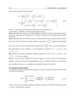
The variation of phase and energy velocity of quasilongitudinal wave is presented in Fig. 6
(a) which shows that the phase velocity does not vary with attenuation angle γ , while the
corresponding energy velocity can be influenced by γ. With γ increasing, the energy velocity
turns small. It is also noted that the phase velocity is a little bigger than the energy velocity
for quasilongitudinal wave mode.
The case of temperature wave is shown in Fig. 6 (b). Different from quasilongitudinal wave,
the phase velocity and energy velocity of temperature wave are influenced by propagation
angle θ and attenuation angle γ. Both phase velocity and energy velocity decay with γ. For
given γ, the phase velocity is also bigger than energy velocity.


244

Heat Conduction – Basic Research
Will-be-set-by-IN-TECH

16

(a)

(b)

Fig. 6. Variations of velocity with propagation angle θ at γ=0◦ , 30◦ .


245
17

Energy Transfer inMaterial
Energy Transfer in Pyroelectric Pyroelectric Material

(a)

(b)

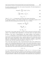
Fig. 7. Variations of velocity with propagation angle θ at γ=0◦ ,30◦ .


246

18

Heat Conduction – Basic Research

Will-be-set-by-IN-TECH

Plots of the computed velocities of quasitransverse wave I and II are given in Fig. 7. The phase
velocities of both wave modes are almost independent of γ and the energy velocity become
small with γ increasing.

4. Conclusion
In this chapter, the energy process of the pyroelectric medium with generalized heat
conduction theory is addressed in the framework of the inhomogeneous wave results
originally. The characters of inhomogeneous waves lie in that its propagation direction
is different from the biggest attenuation direction. The complex-valued wave vector is
determined by four parameters. The range of attenuation angle should be confined in
(-90◦ ,90◦ ) to make waves attenuate. Further analysis demonstrates that, in anisotropic plane,
the positive and negative attenuation angle have different influences on waves, while, in the
isotropic plane, they are the same. Based on the governing equations and state equations, the
dynamic energy conservation law is derived. The energy transfer, in an arbitrary instant, is
described explicitly by the energy conservation relation. From this relation, it is found that
energy density in pyroelectric medium consists of the electric energy density, the heat energy
density, the mechanical potential energy density, the kinetic energy density. The heat loss or
dissipation energy is equal to the reduction of the entire energy within a fixed volume plus
the reduction of this energy flux outward the surface bounding this volume. The dissipation
energy in pyroelectric medium are attributed by the heat conduction, relaxation time and
pyroelectric effect. The energy flux is obtained and it can not be influenced by the relaxation
time. The phase velocity and energy velocity of four wave modes in pyroelectric medium
are studied. Results demonstrate that the attenuation angle almost doesn’t influence phase
velocity of quasilongitudinal, quasitransverse I, II wave modes, while plays large role on
the temperature wave. The energy velocities of the four wave modes all decay with the
attenuation angle.

5. References

Auld, B. A. (1973). Acoustic fields and waves in solids, John Wiley & Sons, New York.
´
Baesu, E., Fortune, D. & Soos, E. (2003). Incremental behaviour of hyperelastic dielectrics and
piezoelectric crystals, Z. angew. Math. Phys. 54: 160–178.
Baljeet, S. (2005). On the theory of generalized thermoelasticity for piezoelectric materials,
Applied Mathematics and Computation 171: 398–405.
Borcherdt, R. D. (1973). Energy and plane waves in linear viscoelastic media, Journal of
Geophysical Research 78(14): 2442–2453.
Buchen, P. W. (1971). Plane waves in linear viscoelastic media, Geophys J R astr Soc 23: 531–542.
Busse, G. (1991). Thermal waves for material inspection, in O. Leroy & M. A. Breazeale (eds),
Physical Acoustics: Fundermentals and Applications, Plenum Press, Kortrijk, Belgium.
Cady, W. G. (1946). Piezoelectricity, An Introduction to the Theory and Applications of
Electromechanical Phenomena in Crystals, McGraw-Hill, New York.
Carcione, J. M. & Cavallini, F. (1997). Forbidden directions for tm waves in anisotropic
conducting media, Antennas and Propagation, IEEE Transactions on 45(1): 133–139.
´
´
Cattaneo, C. (1958). Sur une forme de l, equationeliminant le paradoxe d, une propagation
´
instantanee, Comptes Rend Acad Sc 247: 431–432.
Cerveny, V. & Psencik, I. (2006). Energy flux in viscoelastic anisotropic media, Geophys. J. Int.
166(3): 1299–1317.


Energy Transfer inMaterial
Energy Transfer in Pyroelectric Pyroelectric Material

247
19

Cuadras, A., Gasulla, M., Ghisla, A. & Ferrari, V. (2006). Energy harvesting from pzt
pyroelectric cells, Instrumentation and Measurement Technology Conference, 2006. IMTC
2006. Proceedings of the IEEE, pp. 1668–1672.
Dalola, S., Ferrari, V. & Marioli, D. (2010). Pyroelectric effect in pzt thick films for thermal
energy harvesting in low-power sensors, Procedia Engineering 5: 685–688.
Deschamps, M., Poiree, B. & Poncelet, O. (1997). Energy velocity of complex harmonic plane
waves in viscous fluids, Wave Motion 25: 51–60.
Eringen, A. C. & Maugin, G. A. (1990). Electrodynamics of continua, Vol. I, Springer-Verlag, New
York.
Fang, J., Frederich, H. & Pilon, L. (2010). Harvesting nanoscale thermal radiation using
pyroelectric materials, Journal of Heat Transfer 132(9): 092701–10.
Fedorov, F. I. (1968). Theory of Elastic Waves in Crystals, Plenum Press, New York.
Gael, S. & et al. (2009). On thermoelectric and pyroelectric energy harvesting, Smart Materials
and Structures 18(12): 125006.
Green, A. E. & Lindsay, K. A. (1972). Thermoelasticity, Journal of Elasticity 2(1): 1–7.
Guyomar, D., Sebald, G., Lefeuvre, E. & Khodayari, A. (2008). Toward heat energy harvesting
using pyroelectric material, Journal of Intelligent Material Systems and Structures .
Hadni, A. (1981). Applications of the pyroelectric effect, J. Phys. E: Sci. Instrum. 14: 1233–1240.
He, T., Tian, X. & Shen, Y. (2002). Two-dimensional generalized thermal shock problem of a
thick piezoelectric plate of infinte extent, Int. J. Eng. Sci. 40: 2249–2264.
Joseph, D. & Preziosi, L. (1989). Heat waves, Reviews of Modern Physics 61: 41–73.
Kaliski, S. (1965). Wave equation of thermoelasticity, Bull. Acad. Pol. Sci., Ser. Sci . Tech.
13: 211–219.
Khodayari, A., Pruvost, S., Sebald, G., Guyomar, D. & Mohammadi, S. (2009). Nonlinear
pyroelectric energy harvesting from relaxor single crystals, Ultrasonics, Ferroelectrics
and Frequency Control, IEEE Transactions on 56(4): 693–699. 0885-3010.
Kiselev, A. P. (1982).
Energy flux of elastic waves, Journal of Mathematical Sciences
19(4): 1372–1375.
Kuang, Z. B. (2002). Nonlinear continuum mechanics, Shanghai Jiaotong University Publishing

House, Shanghai.
Kuang, Z. B. (2009).
Variational principles for generalized dynamical theory of
thermopiezoelectricity, Acta Mechanica 203(1): 1–11.
Kuang, Z. B. (2010). Variational principles for generalized thermodiffusion theory in
pyroelectricity, Acta Mechanica 214(3): 275–289.
Kuang, Z. & Yuan, X. (2010). Reflection and transmission of waves in pyroelectric and
piezoelectric materials, Journal of Sound and Vibration 330(6): 1111–1120.
Lord, H. W. & Shulman, Y. (1967). A generalized dynamical theory of thermoelasiticity, J.
Mech. Phys. Solids 15: 299–309.
Mainardi, F. (1973). On energy velocity of viscoelastic waves, Lettere Al Nuovo Cimento
(1971-1985) 6: 443–449.
Majhi, M. C. (1995). Discontinuities in generalized thermoelastic wave propagation in a
semi-infinite piezoelectric rod, J. Tech. Phys 36: 269–278.
Nelson, D. F. (1979). Electric, Optic and Acoustic Interactions in Dielectrics, John Wiley, New
York.
Olsen, R. B., Bruno, D. A., Briscoe, J. M. & Dullea, J. (1984). Cascaded pyroelectric energy
converter, Ferroelectrics 59(1): 205–219.


248

20

Heat Conduction – Basic Research
Will-be-set-by-IN-TECH

Olsen, R. B. & Evans, D. (1983).
Pyroelectric energy conversion: Hysteresis loss
and temperature sensitivity of a ferroelectric material, Journal of Applied Physics

54(10): 5941–5944.
Sharma, J. N. & Kumar, M. (2000). Plane harmonic waves in piezo-thermoelastic materials,
Indian J. Eng. Mater. Sci. 7: 434–442.
Sharma, J. N. & Pal, M. (2004). Propagation of lamb waves in a transversely isotropic
piezothermoelastic plate, Journal of Sound and Vibration 270(4-5): 587–610.
Sharma, J. N. & Walia, V. (2007).
Further investigations on rayleigh waves in
piezothermoelastic materials, Journal of Sound and Vibration 301(1-2): 189–206.
Shen, D., Choe, S.-Y. & Kim, D.-J. (2007). Analysis of piezoelectric materials for energy
harvesting devices under high-igi vibrations, Japanese Journal of Applied Physics
46(10A): 6755.
Sodano, H. A., Inman, D. J. & Park, G. (2005). Comparison of piezoelectric energy harvesting
devices for recharging batteries, Journal of Intelligent Material Systems and Structures
16(10): 799–807.
Umov, N. A. (1874). The equations of motion of the energy in bodies[in Russian], Odessa.
´
´
Vernotte, P. (1958). Les paradoxes de la theorie continue de l, equation de la chaleur, Comptes
Rend Acad Sc 246: 3154.
Xie, J., Mane, X. P., Green, C. W., Mossi, K. M. & Leang, K. K. (2009). Performance of
thin piezoelectric materials for pyroelectric energy harvesting, Journal of Intelligent
Material Systems and Structures .
Yuan, X. (2009). Wave theory in pyroeletric medium, PhD thesis, Shanghai Jiaotong university.
Yuan, X. (2010). The energy process of pyroelectric medium, Journal of Thermal Stresses
33(5): 413–426.
Yuan, X. & Kuang, Z. (2008).
Waves in pyroelectrics, Journal of Thermal Stresses
31(12): 1190–1211.
Yuan, X. & Kuang, Z. (2010). The inhomogeneous waves in pyroelectrics, Journal of Thermal
Stresses 33: 172–186.

11
Steady-State Heat Transfer and Thermo-Elastic
Analysis of Inhomogeneous Semi-Infinite Solids
1Pidstryhach

Yuriy Tokovyy1 and Chien-Ching Ma2

Institute for Applied Problems of Mechanics and Mathematics
National Academy of Sciences of Ukraine, Lviv,
2Department of Mechanical Engineering, National Taiwan University
Taipei
1Ukraine
2Taiwan ROC

1. Introduction
The advancement in efficient modeling and methodology for thermoelastic analysis of
structure members requires a variety of the material characteristics to be taken into
consideration. Due to the critical importance of such analysis for adequate determination of
operational performance of structures, it presents a great deal of interest for scientists in both
academia and industry. However, the assumption that the material properties depend on
spatial coordinates (material inhomogeneity) presents a major challenge for analytical
treatment of relevant heat conduction and thermoelasticity problems. The main difficulty lies
in the need to solve the governing equations in the differential form with variable coefficients
which are not pre-given for arbitrary dependence of thermo-physical and thermo-elastic
material properties on the coordinate. Particularly, for functionally graded materials, whose
properties vary continuously from one surface to another, it is impossible, except for few
particular cases, to solve the mentioned problems analytically (Tanigawa, 1995). The analytical,
semi-analytical, and numerical methods for solving the heat conduction and thermoelasticity

problems in inhomogeneous solids attract considerable attention in recent years. The overview
of the relevant literature is given in our publications (Tokovyy & Ma, 2008, 2008a, 2009, 2009a).
On the other hand, determination of temperature gradients, stresses and deformations is
usually an intermediate step of a complex engineering investigation. Therefore analytical
methods are of particular importance representing the solutions in a most convenient form.
The great many of existing analytical methods are developed for particular cases of
inhomogeneity (e.g., in the form of power or exponential functions of a coordinate, etc.). The
methods applicable for wider ranges of material properties are oriented mostly on
representation the inhomogeneous solid as a composite consisting of tailored homogeneous
layers. However, such approaches are inconvenient for applying to inhomogeneous materials
with large gradients of inhomogeneity due to the weak convergence of the solution with
increasing the number of layers.
A general method for solution of the elasticity and thermoelasticity problems in terms of
stresses has been developed by Prof. Vihak (Vigak) and his followers in (Vihak, 1996; Vihak


250

Heat Conduction – Basic Research

et al., 1998, 2001, 2002; Vigak, 1999; Vigak & Rychagivskii, 2000, 2002). The method consists
in construction of analytical solutions to the problems of thermoelasticity based on direct
integration of the original equilibrium and compatibility equations. Originally the
equilibrium equations are in terms of stresses, and they do not depend on the physical
stress-strain relations, as well as on the material properties. At the same time the general
equilibrium relates all the stress-tensor components. This enables one to express all the
stresses in terms of the governing stresses. The compatibility equations in terms of strain are
then reduced to the governing equations for the governing stresses. When these equations
are solved, all the stress-tensor components can be found by means of the aforementioned
expressions. In addition, the method enables the derivation of: a) fundamental integral

equilibrium and compatibility conditions for the imposed thermal and mechanical loadings
and the stresses and strains; b) one-to-one relations between the stress-tensor and
displacement-vector components. Therefore, when the stress-tensor components are found,
then the displacement-vector components are also found automatically. Such relations have
been derived for the case of one-dimensional problem for a thermoelastic hollow cylinder
(Vigak, 1999a) and plane problems for elastic and thermoelastic semi-plane (Vihak &
Rychahivskyy, 2001; Vigak, 2004; Rychahivskyy & Tokovyy, 2008).
Since application of this method rests upon the direct integration of the equilibrium
equations, the proposed solution scheme offers ample opportunities for efficient analysis of
inhomogeneous solids. In contrast to homogeneous materials, the compatibility equations in
terms of stresses are with variable coefficients. This causes that the governing equations,
obtained on the basis of the compatibility ones, appear as integral equations of Volterra
type. By following this solution strategy, the one-dimensional thermoelasticity problem for a
radially-inhomogeneous cylinder has been analyzed (Vihak & Kalyniak, 1999; Kalynyak,
2000). In the same manner, the two-dimensional elasticity and thermoelasticity problems for
inhomogeneous cylinders, strips, planes and semi-planes were solved in (Tokovyy &
Rychahivskyy, 2005; Tokovyy & Ma, 2008, 2008a, 2009, 2009a). The same method has also
been extended for three-dimensional problems (Tokovyy & Ma, 2010, 2010a). Application of
this method for analysis of inhomogeneous solids exhibits several advantages. First of all,
this method is unified for various kinds of inhomogeneity and different shape of domain
and it does not impose any restriction on the material properties. Moreover, when applying
the resolvent-kernel algorithm for solution of the governing Volterra-type integral equation,
the solutions of corresponding elasticity and thermoelasticity problems for inhomogeneous
solids appear in the form of explicit functional dependences on the thermal and mechanical
loadings, which makes them to be rather usable for complex engineering analysis.
Herein, we consider an application of the direct integration method for analysis of
thermoelastic response of an inhomogeneous semi-plane within the framework of linear
uncoupled thermoelasticity (Nowacki, 1962). The solution of this problem consists of two
stages: i) solution of the in-plane steady-state heat conduction problem under certain
boundary conditions, and ii) solution of the plane thermal stress problem due to the above

determined temperature field and appropriate boundary conditions. Solution of both
problems is reduced to the governing Volterra integral equation. By making use of the
resolvent-kernel solution technique, the governing equation is solved and the solution of the
original problem is presented in an explicit form. Due to the later result, the one-to-one
relationships are set up between the tractions and displacements on the boundary of the
inhomogeneous semi-plane. Using these relations and the solution in terms of stresses, we
find solutions for the boundary value problems with displacements or mixed conditions


Steady-State Heat Transfer and Thermo-Elastic Analysis of Inhomogeneous Semi-Infinite Solids

251

imposed on the boundary. It is shown that these solutions are correct if the tractions satisfy
the necessary equilibrium conditions, the displacements meet the integral compatibility
conditions, and the heat sources and heat flows satisfy the integral condition of thermal
balance.

2. Analysis of the steady-state heat conduction problem in an
inhomogeneous semi-plane
In this section, we consider an application of the direct integration method for solution of the
in-plane steady-state (stationary) heat conduction problem for a semi-plane whose thermal
conductivity is an arbitrary function of the depth-coordinate. Having applied the Fourier
integral transformation to the differential heat conduction equation with variable coefficients,
this equation is reduced to the Volterra-type integral equation, which then is solved by making
use of the resolvent-kernel technique. As a result, the temperature distribution is found in an
explicit functional form that can be efficiently used for analysis of thermal stresses and
displacements in the semi-plane.
2.1 Formulation of the heat conduction problem
Let us consider the two-dimensional heat conduction problem for semi-plane

D  {( x , y )  (  ,  )  [0,  )} in the dimensionless Cartesian coordinate system (x, y). In
assumption of the isotropic material properties, the problem is governed by the following
heat conduction equation (Hetnarski & Reza Eslami, 2008)
T ( x , y )   
T ( x , y ) 
 
 k( y ) x   y  k( y ) y   q( x , y ),
x 




(1)

where T ( x , y ) is the steady-state temperature distribution, k(y) stands for the coefficient of
thermal conduction, and q(x, y) denotes the quantity of heat generated by internal heat
sources in semi-plane D. When the coefficient of thermal conduction is constant, then
equation (1) presents the classical equation of quasi-static heat conduction (Nowacki, 1962;
Carslaw & Jaeger, 1959)
T ( x , y )   W ( x , y ),

(2)

where    2 /x 2   2 /y 2 and W ( x , y )  q( x , y ) / k denotes the density of internal sources

of heat. In the steady-state case, the temperature T ( x , y ) can be determined from equation
(1) for k( y ) or (2) for k  const under certain boundary condition imposed at y  0
(Nowacki, 1962). We consider the boundary condition in one of the following forms:
a. the temperature distribution is prescribed on the boundary
T ( x , y )  T0 ( x ), y  0;

b.

(3)

the heat flux over the limiting line y  0 is prescribed on the boundary
T ( x , y )
  0 ( x ), y  0;
y

(4)


252

c.

Heat Conduction – Basic Research

the heat exchange condition is imposed on the boundary
T ( x , y )
  0T ( x , y )   0 , y  0.
y

(5)

Here  0 and  0 are constants, T0 ( x ) and  0 ( x ) are given functions. Assuming that the
temperature field, heat fluxes, and the density of heat sources vanish with |x|, y   , we
consider finding the solution to equation (1) or (2) under either of the boundary conditions
(3) – (5) and the supplementary conditions of integrability of the functions in question in

their domain of definition.
2.2 Solution of the stated heat conduction problem by reducing to the Volterra-type
integral equation
In the case when k  const , it has been shown (Rychahivskyy & Tokovyy, 2008) that for
construction of a correct solution to equation (2) with boundary condition (4), the following
necessary condition


D W (x , y )dxdy   0 ( x)dx

(6)

is to be fulfilled. This condition of thermal balance postulates that the resultant heat flux
trough the boundary y  0 is equal to the resultant action of internal heat sources within
domain D. In the case of boundary conditions (3) or (5), the right-hand side of condition (6)
should be replaced by the integral of the heat flux at y  0 , which is determined by the
temperature. Due to this reason, condition (6) can be regarded as an efficient tool for
verification of the solution correctness.
Note that condition (6) is natural for steady-state thermal processes in bounded solids.
However, it is not intuitive for non-stationary thermal regimes since then only certain
distribution of the temperature field is possible inside the solid implying that the heating of
the solid until an average temperature is not achievable. Thus, condition (6) for a semi-plane
is a consequence of application of solid mechanics to the oversimplified geometrical model.
By denoting
 x ( x , y )  k( y )
in

equation

(1),

when

T( x , y )
T ( x , y )
,  y ( x , y )  k( y )
x
y

k  k( y ) ,

and

following

the

strategy

presented

in

(Rychahivskyy & Tokovyy, 2008), it can be shown that condition (6) holds for the case of
inhomogeneous material. In addition, the resultant of the temperature is necessarily equal to
zero

D T ( x , y )dxdy  0

(7)

for both homogeneous and inhomogeneous cases.
Let us construct the solution to equation (1) under boundary conditions (3), (4), or (5) by
taking conditions (6) and (7) into consideration. Having applied the Fourier integral
transformation (Brychkov & Prudnikov, 1989)


Steady-State Heat Transfer and Thermo-Elastic Analysis of Inhomogeneous Semi-Infinite Solids

f ( y ; s)  





f ( x , y )exp( isx )dx

253

(8)

to the aforementioned equation and boundary conditions, we arrive at the following second
order ODE
d2 T ( y ; s)
d y2

 s 2T ( y ; s )  

d k( y ) d T ( y ; s ) 
1 

 q ( y ; s) 

k( y ) 
dy
dy 

(9)

that is accompanied with one of the following boundary conditions:

T ( y ; s)  T0 (s ), y  0;

(10)

d T ( y ; s)
  0 (s ), y  0;
dy

(11)

d T ( y ; s)
  0T ( y ; s )   0 , y  0.
dy

(12)

Here s is a parameter of the integral transformation, i 2  1 , f  x , y   L  D  . For the sake of
brevity, the parameter s will be omitted from the arguments of functions in the following
text.
A general solution to equation (9) in semi-plane D can be given in the form

T ( y )  C exp( |s|y ) 



1  q ( )
exp( |s|| y   |)d
2|s|0 k( )

1  1 d k( ) d T ( )
exp( |s|| y   |)d ,
2|s|0 k( ) d
d

(13)

where C is a constant of integration and || denotes the absolute-value function. By
applying the integration by parts to the last integral in equation (13), we can obtain the
following Volterra-type integral equation of second kind:



T (0) dk(0) 
T(y)  C 
 exp( |s|y )  q*( y )  0 T ( )K ( y , )d .
2|s|k(0) dy 

Here

q*( y ) 

K( y , )  

1  q ( )
exp( |s||y   |)d ,
2|s|0 k( )


1 d  1 dk( )
exp( |s|| y   |) 

2|s|d  k( ) d


(14)


254

Heat Conduction – Basic Research



 dk( ) d 2 k( )  exp( |s||y   |)
1   1 dk( )
|s|sgn( y   ) 

.


2|s|  k( ) d

k( )
d 2 
 d



(15)

To solve integral equation (14), different algorithms can be employed, for instance, the
Picard’s process of successive approximations (Tricomi, 1957; Kalynyak, 2000;
Tokovyy & Ma, 2008a), the operator series method (Bartoshevich, 1975), the BubnovGalerkin method (Fedotkin et al., 1983), a numerical procedure based on trapezoidal
integration and a Newton-Raphson method (Frankel, 1991), iterative-collocation method
(Hącia, 2007), discretization method, special kernels method and projection-iterative method
(Domke & Hącia, 2007), spline approximations (Kushnir et al., 2002), the quadratic-form
method (Belik et al. 2008), the greed methods (Peng & Li, 2010). Herein we employ the
resolvent-kernel algorithm (Pogorzelski, 1966; Porter & Stirling, 1990) in the same manner as
it has been done in (Tokovyy & Ma, 2008, 2009a). This method allows us to obtain the
explicit-form analytical solution that is convenient for analysis. As a result, the
transformation of temperature appears as

T (0) dk(0) 
T(y)  C 
  ( y )   ( y ),
2|s|k(0) dy 


(16)

where


 ( y )  exp( |s|y )   exp( |s| )( y , )d ,
0



 ( y )  q*( y )   q*( )( y , )d ,
0

(17)

(18)

and the resolvent-kernel is determined by the recurring kernels as
( y , ) 



 Kn  1 ( y , ),

n0

(19)



K 1 ( y , )  K ( y , ), K n  1 ( y , )   K ( y ,  )K n ( , )d , n  1, 2,...
0

Note that expression (16) is advantageous in comparison with the analogous solutions

constructed by means of the aforementioned techniques for solution of the Volterra integral
equations. First of all, solution (16) is obtained in explicit functional form. This fact can be
efficiently used for complex analysis involving solution of thermoelasticity problem. Next,
the resolvent (19) is expressed only through the kernel (15) of integral equation (14)
(“intrinsic” properties of an integral equation) and is non-dependent of the free term
(“external” properties of an integral equation). Consequently, being computed once for
certain kernel (which means for certain material properties, obviously), resolvent (19) can be
employed for various kinds of thermal loading.
To determine the unknown constant C in equation (16), one of conditions (10) – (12) should
be employed. Insertion of (16) into condition (10) yields


Steady-State Heat Transfer and Thermo-Elastic Analysis of Inhomogeneous Semi-Infinite Solids

C

255

T0 
 (0) dk(0)   (0)
,
1 

 (0) 
2|s| k(0) dy   (0)

and then the temperature can be given as
T(y) 

T0   (0)

 ( y )   ( y ).
 (0)

(20)

In the case of boundary condition (11), the constant C appears as
 d (0) 
C  q0 

 dy 

1

1



T (0) dk(0) d (0)  d (0) 


 .
2|s| k(0) dy
dy  dy 

Then the temperature can be given as
1


d (0)  d (0) 
T ( y )   q0 


  ( y )   ( y ).
dy  dy 


(21)

In the case of boundary condition (12), the constant C takes the form

d (0) 
d (0) 
C    0   0 (0) 
  0 (0) 

dy 
dy 


1



T (0) dk(0)
,
2|s|k(0) dy

and, consequently,
1



d (0) 
d (0) 
T ( y )    0   0 (0) 
  0 (0) 
  ( y )   ( y ).
dy 
dy 


(22)

Having determined the expressions for the temperature field in the form (20), (21), or (22)
and applying the formula
f (x , y ) 

1
2





f ( y ; s )exp(isx )ds

(23)



of inverse Fourier transformation (Brychkov & Prudnikov, 1989), we can obtain the
expressions for temperature field in semi-plane D.

Note that according to the resolvent-kernel theory (Verlan & Sizikov, 1986), the recurring
kernels K n  1 tend to zero as n   . Thus, for practical computations, the series in
expression (19) can be truncated. Consequently,
( y , )  N ( y , ) 

N

 Kn 1 ( y , ),

n0

where N is a natural number which depends on required accuracy of calculation.

(24)


256

Heat Conduction – Basic Research

2.3 Numerical analysis
To verify the obtained solution to the heat conduction problem, let us examine the case,
when the semi-plane is heated by a single concentrated internal heat source
q( x , y )  q0 ( x ) ( y  y 0 ).

(25)

Meanwhile the boundary y  0 remains of the constant temperature, T0  0 . Here q0 is a
constant dimensional parameter;  () denotes the Dirac delta-function. In this case, the
temperature should be computed on the basis of expression (20). The coefficient of thermal

conductivity is assumed to be in the following form
k( y )  k0 exp( y ),

(26)

where k0 and  are constants. Note that for   0 , the thermal conductivity in the form
(26) is constant, that corresponds to the case of homogeneous material. Then, on the basis of
expression (19), the resolvent ( y , )  0 and thus expression (20) presents an exact

analytical solution
T ( y ) k0
1

 exp( |s||y  y0 |)  exp( |s|( y  y0 )) .
q0
2|s|

(27)

Application of the Fourier inversion (23) to formula (27) yields the expression for the
temperature in the homogeneous semi-plane, as follows:
x 2  ( y  y0 )2
k0
1
ln 2
.
T (x , y ) 
q0
4 x  ( y  y0 )2

(28)

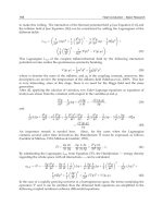
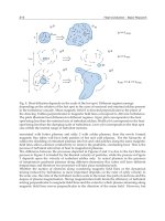
The full-field distributions of the temperature (28) and the components of corresponding
heat flux are depicted in Fig. 1 for y0  1 . Distribution of the temperature (28) versus the

Fig. 1. Full-field distributions of (a) the dimensionless temperature
versal

k0T ( x , y )
, and (b) transq0

k0 T ( x , y )
k T ( x , y )
and (c) longitudinal 0
components of the heat flux for y0  1
y
x
q0
q0


Steady-State Heat Transfer and Thermo-Elastic Analysis of Inhomogeneous Semi-Infinite Solids

257

variable y is shown in Fig. 2 for x = 0.0; 0.5 and different values y0  1.0; 2.0; 3.0; 4.0. As we
can observe in both figures, the thermal state is symmetrical with respect to the line x  0 .
The temperature vanish when mowing away from the location of the heat source (0, y0 ) .
When approaching the boundary y  0 , the temperature vanish faster than in the opposite
direction (due to satisfaction of the boundary condition). When the location of the heat

source is moving away from the boundary, then the thermal state tends to one symmetrical
with respect to the line y  y0 (Fig. 2) due to the lowering influence of the boundary (in
analogy to the case of an infinite plane).

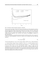
Fig. 2. Distribution of the temperature (28) versus coordinate y for x  0.0;0.5

Fig. 3. The heat flux (29) for different values of y 0  1.0; 2.0; 3.0; 4.0

Fig. 4. Dependence of the thermal conductivity on the coordinate y for different values of 
For the obtained temperature, the heat flux trough the boundary y  0 can be found as


258

Heat Conduction – Basic Research

y
k0  0
 2 02 .
q0
( x  y0 )

(29)

By taking formulae (25) and (29) into consideration, it is easy to see that condition (6) is
satisfied for the considered case. Distribution of the heat flux (29) for different values of y 0 is
shown in Fig. 3. As we can see, the heat flux over the boundary is locally distributed with the
maximum value at x  0 which decreases as the heat source is further from the boundary.
Now let   0 in (26). For this case, the exact solution can be constructed by following the
technique presented in (Ma & Lee, 2009; Ma & Chen, 2011). According to this technique, the

exact solution to the problem (1), (3), (25) can be found in the form

 
 







 
 




 exp y   /2  exp  y   /2 exp  y  /2 , y  y ,
0
0
0
q0
k0

T(y)  

2
2




q0
  4s  exp y /2  exp  y /2 exp  y0 /2 , y  y0 ,


(30)

where     2  4s 2   . To obtain the distribution of temperature due to Fourier
transform (30), the inversion formula (23) can be applied. The distributions of obtained
temperature and corresponding heat flux are examined for different values of the parameter
of inhomogeneity:   1 ,   1 , and, for comparison with above-discussed homogeneous
case,   0 (Fig. 4). For   1 , the thermal conductivity grows exponentially from 1 to
infinity; for   1 it decreases from 1 to 0.

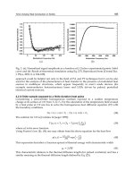
Fig. 5. Distribution of the temperature due to transformant (30) versus coordinate y at
x  0.0 for   0, 1

Fig. 6. Distribution of the heat flux across the boundary y  0 for y 0  1.0; 3.0 ,   0; 1


Steady-State Heat Transfer and Thermo-Elastic Analysis of Inhomogeneous Semi-Infinite Solids

259

Fig. 7. Distribution of the heat flux for y 0  1.0; 3.0 ,   0, 1
The effect of inhomogeneity on the temperature and heat flux over the boundary y  0 is
shown in Figs. 5 and 6, respectively. As we observe in Fig. 5, the temperature vanishes with
y   as faster as the parameter of inhomogeneity  is greater, whereas for 0  y  y0
vice-verse. Consequently, the heat flux over the boundary y  0 is greater for greater
values of  (Fig. 6).

Now we consider application of formula (20) for computation of the temperature in the
inhomogeneous semi-plane. We employ formula (24) instead of (19) in (17) and (18).
Distribution of the temperature computed by formula (20) for different values of parameter
N in (24) is shown in Fig. 7. With growing N, the result naturally tends to the exact solution
(30) and for N  5 they coincide. This result shows that expression (24) provides sufficiently
good approximation for the resolvent ( y , ) by holding few terms only.

3. Analysis of thermal stresses in an inhomogeneous semi-plane
In this section, the technique for solving the plane thermoelasticity problem for an isotropic
inhomogeneous semi-plane with boundary conditions for stresses or displacements, as well
as mixed boundary conditions, is developed by establishing one-to-one relations between
boundary tractions and displacements. This technique is based on integration of the Cauchy
relations to express displacements in terms of strains. Then, by taking the physical strainstress relations into consideration, the displacements are expressed through the stress-tensor
components. Finally, by making use of the explicit-form analytical solution to the
corresponding problem with boundary tractions, the displacements on the boundary can be
expressed through the tractions. The technique for establishment of the one-to-one relations
between the tractions and displacements on the boundary, as well as for deriving the
necessary equilibrium and compatibility conditions in the case of homogeneous semi-plane
has been developed in (Rychahivskyy & Tokovyy, 2008).
3.1 Formulation of the problem
Let us consider the plane quasi-static thermoelasticity problem in inhomogeneous semiplane D . In absence of body forces, this problem is governed (Nowacki, 1962) by the
equilibrium equations
 x ( x , y )  xy ( x , y )

 0,
x
y

 xy ( x , y )
x



 y ( x , y )
y

 0,

(31)


260

Heat Conduction – Basic Research

the compatibility equation in terms of strains
 2 x ( x , y )
y 2



 2 y ( x , y )
x 2



 2 xy ( x , y )
xy

,

(32)

the physical thermoelasticity relations

 x (x, y ) 

 * (y)
1
 x (x, y ) 
 y ( x , y )   *( y )T ( x , y ),
E* ( y )
E* ( y )

 y (x , y ) 

 * (y)
1
 y (x , y ) 
 x ( x , y )   *( y )T ( x , y ),
E* ( y )
E* ( y )
 xy ( x , y ) 

(33)

1
 xy ( x , y ),
G( y )

and the geometrical Cauchy relations

 x (x, y ) 
Here  x , y , xy
respectively;

and

u( x , y )
v( x , y )
u( x , y ) v( x , y )
, y 
,  xy 

.
x
y
y
x

 x ,  y ,  xy

(34)

denote the stress- and strain-tensor components,

 E( y )
  (y)
, plane strain,
, plane strain,



E* ( y )   1   2 ( y )
 * ( y )   1  ( y )
 E( y ),
  ( y ),
plane stress,
plane stress,


 ( y )(1   ( y )), plane strain,
* (y)  
plane stress,
 ( y ),

E( y )
is the
2(1   ( y ))
shear modulus,  ( y ) denotes the coefficient of linear thermal expansion; u( x , y ) and
v( x , y ) are the dimensionless displacements; T ( x , y ) is the temperature field that is given or
determined in the form (20), (21), or (22) by means of the technique proposed in the previous
section.
We shall construct the solutions of the set of equations (31)–(34) for each of the three
versions of boundary conditions prescribed on the line y  0 :
a. in terms of stresses
E(y) denotes the Young modulus,  ( y ) stands for the Poisson ratio; G( y ) 

 y ( x , y )   p( x ),
b.

 xy ( x , y )  q( x ),

y  0;

(35)

in terms of displacements

u( x , y )  u0 ( x ),

v( x , y )  v0 ( x ),

y  0;

(36)


261

Steady-State Heat Transfer and Thermo-Elastic Analysis of Inhomogeneous Semi-Infinite Solids

c.

mixed conditions, when one of the following couples of relations

 y ( x , y )   p( x ), v( x , y )  v0 ( x ), y  0;
 y ( x ,0)   p( x ), v( x ,0)  v0 ( x ), y  0;

(37)

 xy ( x ,0)  q( x ), u( x ,0)  u0 ( x ), y  0;
 xy ( x ,0)  q( x ), v( x ,0)  v0 ( x ), y  0

is imposed on the boundary. The boundary tractions and displacements, those are
mentioned in conditions (35)—(37), as well the temperature field, vanish with |x|  ,

y   . We consider finding the solutions (stresses and displacements) of the stated
boundary value problems.
3.2 Construction of the solutions
3.2.1 Case A: Boundary condition in terms of external tractions
Let us consider the construction of solution to the problem (31) – ( 34) under boundary
conditions (35) with given tractions p( x ) and q( x ) . The boundary displacements u0 ( x ) and
v( x ) are unknown and, thus, they should be determined in the process of solution. By
following the solution strategy (Tokovyy & Ma, 2009), the stress-tensor components can be
expressed trough the in-plane total stress    x   y as

x   y ,

 xy

|s| 
 y   p exp( |s|y ) 
 ( )  exp( |s||y   |)  exp( |s|( y   )) d ,
(38)
2 0
i|s|
is 

p exp( |s|y )    ( )  exp( |s||y   |)sgn( y   )  exp( |s|( y   )) d .
s

2 0

In turn, the total stress can be found as a solution of the Volterra-type integral equation of
second kind:

 ( y )  E* ( y )  pP( y )  A exp( |s| y )   * ( y )T ( y )    ( )M( y , )d ,


(39)

0

where
M( y , )  

E* ( y )  d 2  1 

 exp  |s||   ||y   |   exp  |s|   |y   |  d ,
8 0 d 2  G( ) 



P( y ) 



1  d2  1 

 exp  |s|( |y   |) d ,
4|s|0 d 2  G( ) 

and the constant of integration A is to be found from the following integral condition


p

0  ( y )exp( |s|y )dy  |s| 

iq
.
s


262

Heat Conduction – Basic Research

To solve equation (39), we employ the resolvent-kernel
(Tokovyy & Ma, 2009a) with the following resolvent
( y , ) 

solution

technique



 N n 1 ( y , ),

n0



N 1 ( y , )  M( y , ), N n  1 ( y , )   M( y ,  )N n ( , )d , n  1, 2,...
0

As a result, the in-plane total stress appears in the form

 ( y )  p( y )  ( y )  Af A ( y ),

(40)

where
A


 iq
1   1
 p
 |s|  (0)   s  (0)  ,

f A (0)  




( y )  E*( y )P( y )   E*( )P( )( y , )d ,
0



( y )   *( y )E*( y )T ( y )    *( )E*( )T ( )( y , )d ,
0



f A ( y )  E*( y )exp( |s| y )   E*( )exp( |s| )( y , )d .
0

Having determined the total stress  by formula (40), the stress-tensor components can be
computed by means of formulae (38). The displacement-vector components u( x , y ) and
v( x , y ) , as well as the boundary displacement u0 ( x ) and v0 ( x ) , can be also determined by

the stresses by means of correct integration of the Cauchy relations (34).
3.2.2 Integration of the Cauchy relations and determination of the displacementvector components in the inhomogeneous semi-plane due to the given boundary
tractions
By taking the boundary conditions (36) with unknown boundary displacements u0 ( x ) and
v0 ( x ) into account, the first and second relations of (34) yield

1 
 x ( , y )sgn( x   )d ,
2 
v
1 
v( x , y )  0    y ( x , )sgn( y   )d .
2 2 0
u( x , y ) 

(41)

By letting x   in the first equation of (41), we derive the integral condition


  x ( x , y )dx  0 ,

(42)


Steady-State Heat Transfer and Thermo-Elastic Analysis of Inhomogeneous Semi-Infinite Solids

263

which is necessary for compatibility of strains. Analogously, by letting y  0 in the second
equation of (41), the condition


0  y ( x , y )dy  v0 ( x )

(43)

can be obtained. By substitution of expressions (41) into the third formula of (34), we derive
following equation
2 xy ( x , y ) 

  x ( , y )
dv0 ( x )

sgn( x   )d

dx

y



  y ( x , )

0

x

sgn( y   )d ,

(44)

which presents the condition of compatibility for strains. It is easy to see that by
differentiation by variables x and y, equation (44) can be reduced to the classical
compatibility equation (32). However, for the equivalence of these two equations, the
following fitting condition
dv0 ( x )
1   x ( ,0)
  xy ( x ,0)  
sgn( x   )d
dx
2  y

(45)

is to be fulfilled. This condition is obtained by integration of equation (32) over x and y with
conditions (36) and (43) in view and comparison of the result to equation (44).
To determine the displacement-vector components, we can employ formulae (41) with

conditions (42), (43), and (45) in view. Having applied the Fourier transformation (8) to the
mentioned equations, we arrive at the formulae
i
u( y )    x ( y ),
s
1 
v ( y )    y ( )  sgn( y   )  1  d .
2 0

(46)

Putting the first and second physical relations of (33) along with (38) and (40) into the
obtained formulae yields the following expressions:
u( y )  p u ( y )  u ( y )  Af u ( y ),
v ( y )  p v ( y )   v ( y )  Af v ( y ),

(47)

where
exp( |s|y ) 
i  ( y )
|s| 
u (y)   

0 ( )  exp( |s||y   |)  exp( |s|( y   )) d  2G( y )  ,
s  E*( y ) 4G( y )


i  ( y )
|s| 

u ( y )   

( )  exp( |s||y   |)  exp( |s|( y   )) d   *( y )T ( y )  ,
s  E*( y ) 4G( y ) 0
