Heat Conduction Basic Research Part 14 ppt

Heat Conduction – Basic Research

314

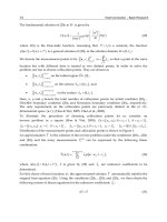
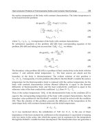
Fig. 23. Temperature distribution along red line for Fig. 22

Maximum temperature (

K
)
1556.70
Averaged kernel temperature ( 
K
)
1518.88
Averaged moderator temperature ( K )
1484.61
Surface temperature at 2.5cm (
K
)
1379.82
Surface temperature at 3.0cm (
K
)
1339.65
Computing time 43h 35m 9s
Table 7. Results for the Fourth Configuration Shown in Fig. 23


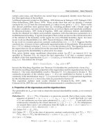
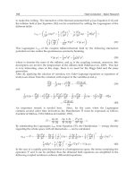
Fig. 24. Cross-sectional views for Fig. 22

Particle Transport Monte Carlo Method for Heat Conduction Problems

315
The temperature profile on the 0

z plane along red line is shown in Fig. 23 and Table 7. In
this FLS model, the maximum fuel temperature appears not at the center point but near the
central region, as the fuels are concentrated on the right side of the center point on
the
0z plane, as shown in Fig. 24. Note that the red circle in Fig. 24 denotes particles with
the dominant effect of the temperature increase on the
0

z plane.
3.2 CLCS (Coarse Lattice with Centered Sphere) model
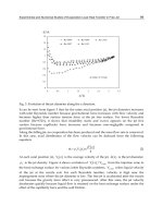
The temperature distribution was obtained again for the CLCS (Coarse Lattice with
Centered Sphere) model [14]. In this model, the tally regions used are shown in Fig. 25. The
general geometry
information is identical to that in Table 2, except that there are 9315 triso particles and each
triso particle takes one lattice cube (and vice versa), as shown in Fig. 26. The resulting
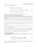
temperature distribution for the CLCS model is shown in Fig. 27.


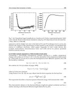
Fig. 25. Tally regions for the CLCS model


Fig. 26. Fuel particle configuration for the CLCS model

Heat Conduction – Basic Research

316

Fig. 27. Results of cubes along red line for Fig. 26
4. Concluding remarks
A Monte Carlo method for heat conduction problems was presented in this chapter. Based
on the asymptotic theory correspondence between neutron transport and diffusion
equations, it is shown that the particle transport Monte Carlo simulation can provide
solutions to the heat conduction problems with two modeling devices introduced: i)
boundary layer correction by the extended problem domain and ii) scaling factor to increase
the diffusivity of the problem.
The Monte Carlo method can be used to solve heat conduction problems with complicated
geometry (e.g. due to the extreme heterogeneity of a fuel pebble in a VHTGR, which houses
many thousands of coated fuel particles randomly distributed in graphite matrix). It can
handle typical boundary conditions, including non-constant temperature boundary
condition and heat convection boundary condition. The HEATON code was written using
MCNP as the major engine to solve these types of heat conduction problems. Monte Carlo
results for randomly sampled configurations of triso fuel particles were presented, showing
the fuel kernel temperatures and graphite matrix temperatures distinctly. The fuel kernel
temperatures can be used for more accurate neutronics calculations in nuclear reactor
design, such as incorporating the Doppler feedback. It was found that the volumetric
analytic solution commonly used in the literature predicts lower temperatures than those of
the Monte Carlo results. Therefore, it will lead to inaccurate prediction of the fuel
temperature under Doppler feedback, which will have important safety implications.
An obvious area of further application is the time transient problem. The results of the
steady-state heterogeneous calculations by Monte Carlo (as described in this chapter) can be
used to construct a two-temperature homogenized model that is then used in transient
analysis [18].
While the Monte Carlo method has its capability and efficacy of handling heat conduction
problems with very complicated geometries, the method has its own shortcomings of the

long computing time and variance due to the statistical results. It also has a limitation in that
it provides temperatures at specific points rather than at the entire temperature field.

Particle Transport Monte Carlo Method for Heat Conduction Problems

317
Appendix A: Elements of Monte Carlo method
A.1 Introduction
In a typical form of the particle transport Monte Carlo method [9,19], we simulate particle
(e.g., neutron) behavior by following a finite number, say
N, of particle histories and tallying
the appropriate events needed to calculate the quantity of interest. The simulation is
performed according to the physical events (expressed by each term in the transport
equation) that a particle would encounter through the use of random numbers. These
random numbers are usually generated by a pseudo random number generator, that
provides uniform random number

between 0 and 1. In each particle history, the random
numbers are generated and used to sample discrete events or continuous variables as the
case may be according to the probability distribution functions. The results of tally are
processed to provide estimates for the mean and variance of the quantity of interest, e.g.,
neutron flux, current, reaction rate, or some other quantities.
A.2 Basic operations of sampling
A.2.1 Sampling of random events
The discrete events such as the type of nuclides and collisions are simple to sample. For
example, suppose that there are in the medium
I nuclides with total macroscopic cross
sections,
(i)
t

,i , , ,I

 12

. Let

I
(i)
tt
i





1
, (A1)
and

(i)
t
i
t
P,i,,,I.


12

(A2)
Now draw a random number


and if

ii
PP P PP P,



 
12 1 12

(A3)
then the
i -th nuclide is selected and the neutron collides with nuclide i . After determination
of the nuclide, the type of collisions (absorption, fission, or scattering, etc.) is determined in
a similar way. If the event is scattering, the energy and direction of the scattered neutron are
sampled. In addition, the distance a neutron travels before suffering its next collision is
sampled. These values are continuous variables and thus determined by sampling according
to the appropriate probability density function
()
f
x . For example, the distance l to next
collision (within the same medium) is distributed as

()



t
l

t
f
ldl e dl
, (A4)
with its cumulative distribution function

t
l
l
F(l) f (l )dl e





0
1
. (A5)
Since
()
F
l is uniformly distributed between 0 and 1, we draw a random number

and let

Heat Conduction – Basic Research

318
F(l)



, (A6)
that in turn provides

tt
ln( ) ln( )
l





 
1
. (A7)
A.2.2 Geometry tracking
In typical Monte Carlo codes, the geometries of the problem are created with intersection
and union of surfaces. In turn, the surfaces are defined by a collection of elementary
mathematical functions. For example, the geometry in Fig. A1 would be defined by
functions that represent four straight lines and a circle.


Fig. A1. An example of problem geometry with two material media


Fig. A2. Geometry tracking
Suppose that the neutron we follow is now at point A and heading to the direction as in Fig.
A2. In order to determine next collision point, first we calculate the distance
1
()l to the

nearest material interface and draw a random number

i
, then two cases occur; i)

Particle Transport Monte Carlo Method for Heat Conduction Problems

319
if
11



t
l
i
e , the collision is in region 1 at point
1
ln /



iit
l , or ii) if
11



t
l

i
e , it says
that the collision is beyond region 1, so draw another random number
1


i
to determine the
collision point that may be in region 2 at
112
ln /




iit
l beyond
1
l along the same
direction. This process continues until the neutron is absorbed or leaks out of the problem
boundary.
A.2.3 Tally of events
To calculate neutron flux of a region, current through a surface, or reaction rate in a region,
the events that are usually tallied are i) number of collisions, ii) total track length traveled, or
iii) number of crossings through a surface. For example, suppose that we like to calculate
average scalar flux

in a volume element V with total cross section

t

. From a well-
known relation,

t
cV


 , (A8)
where
c
is the number of collisions made by neutrons inV , we can calculate

by tallying
the number of collisions:

t
c
V



1
. (A9)
We provide sample estimate of
c by

N
n
n
ˆ

cc
N



1
1
, (A10)
where
n
c is the number of collisions made inV during the n-th history and N is a large
number. In addition, we also provide sample estimate of variance on
c by


N
n
n
N
n
ˆ
S(cc)
N
N
ˆ
(c c ),
N









22
1
22
1
1
1
1
(A11)
where


N
n
n
cs
N



22
1
1
. (A12)
It can be easily shown that the sample standard deviation on
ˆ

c is

ˆ
c
S
N


, (A13)

Heat Conduction – Basic Research

320
which suggests to use a large N for accurate
ˆ
c
, since
ˆ

c
is a measure of uncertainty in the
estimated
ˆ
c
.
Fig. A3 shows an example for
n
c ; in the shaded region,
c,c,c,andc,


 
123 4
011 3
thus
ˆ
c
ˆ
c.,
S(.).,
.



  

22
1
5125
4
311
1 25 1 583
44
1 583
0 6291
4



Fig. A3. Tally of number of collisions
Appendix B: Derivation of equivalent thermal conductivities

The expressions of
2
k (equivalent thermal conductivity) for the convective medium are
derived in this Appendix for three (sphere, cylinder, slab) geometries.
B.1 Sphere geometry
The heat conduction equation in spherical coordinates is, in a region free of heat source,

kd dT
r.
dr dr
r

2
2
2
0
(B1)

Particle Transport Monte Carlo Method for Heat Conduction Problems

321
Thus,

dT
rc,
dr

2
1
(B2)

dT c
,
dr
r

1
2
(B3)

c
Tc.
r
 
1
2
(B4)
From Eq. (B4),

sb
sb
bs sb
rr
TT c c ,
rr rr


  



11
11
(B5)
and thus

sb
sb
sb
rr
c(TT),
rr


1
(B6)
The convective boundary condition equation for spherical geometry is,

s
sb
r
dT
kh(TT).
dr

2
(B7)
Substituting Eqs. (B3) and (B6) into (B7), we have

s
bs

b
r
kh(rr) .
r




2
(B8)
B.2 Cylinder geometry
The heat conduction equation in cylindrical coordinates is, in a region free of heat source,

kddT
r.
rdr dr

2
0
(B9)
Thus,

dT
rc,
dr

1
(B10)

dT c

,
dr r

1
(B11)

Tclnrc,


12
(B12)
From Eq. (B12),

Heat Conduction – Basic Research

322

s
sb s b
b
r
T T c (lnr lnr ) c ln ,
r

  


11
(B13)
and thus

sb
sb
TT
c.
ln(r / r )


1
(B14)
The convective boundary condition equation for cylindrical geometry is,

s
sb
r
dT
kh(TT).
dr

2
(B15)
Substituting Eqs. (B11) and (B14) into (B15), we have

b
s
s
r
khrln .
r





2
(B16)
B.3 Slab geometry
The heat conduction equation in slab geometry is, in a region free of heat source,

dT
k.
dx

2
2
2
0 (B17)
Thus,

dT
c,
dx

1
(B18)

Tcxc,


12
(B19)

From Eq. (B19),

sb sb
TT c(xx), 
1
(B20)
and thus

sb
sb
TT
c,
xx



1
(B21)
The convection boundary condition equation for slab geometry is,

s
sb
r
dT
kh(TT).
dr

2
(B22)
Substituting Eqs. (B18) and (B21) into (B22), we have

bs
kh(xx).
2
(B23)

Particle Transport Monte Carlo Method for Heat Conduction Problems

323
5. References
[1] H.S. Carslaw and J.C. Jaeger, Conduction of Heat in Solids, 2
nd
ed., Oxford (1959).
[2]
T.M. Shih, Numerical Heat Transfer, Hemisphere Pub. Corp., Washington, D.C. (1984).
[3]
S.V. Patankar, Numerical Heat Transfer and Fluid Flow, McGraw-Hill, New York (1980).
[4]
P.E. MacDonald, et al, “NGNP Point Design–Results of the Initial Neutronics and
Thermal-Hydraulic Assessments During FY-03”, Idaho Natural Engineering and
Environmental Laboratory, INEEL/EXT-03-00870 Rev. 1, September (2003).
[5]
James J. Duderstadt and Louis J. Hamilton, Nuclear Reactor Analysis, John Wiley & Sons,
Inc. (1976).
[6]
Jun Shentu, Sunghwan Yun, and Nam Zin Cho, “A Monte Carlo Method for Solving
Heat Conduction Problems with Complicated Geometry,” Nuclear Engineering and
Technology, 39, 207 (2007).
[7]
Jae Hoon Song and Nam Zin Cho, “An Improved Monte Carlo Method Applied to the

Heat Conduction Analysis of a Pebble with Dispersed Fuel Particles,” Nuclear
Engineering and Technology, 41, 279 (2009).
[8]
Bum Hee Cho and Nam Zin Cho, "Monte Carlo Method Extended to Heat Transfer
Problems with Non-Constant Temperature and Convection Boundary Conditions,"
Nuclear Engineering and Technology, 42, 65 (2010).
[9]
X-5 Monte Carlo Team, “MCNP – A General Monte Carlo N-Particle Transfer Code,
Version 5(Revised)”, Los Alamos National Laboratory, LA_UR-03-1987 (2008).
[10]
T.J. Hoffman and N.E. Bands, “Monte Carlo Surface Density Solution to the Dirichlet
Heat Transfer Problem”, Nuclear Science and Engineering, 59, 205-214 (1976).
[11]
A. Haji-Sheikh and E.M. Sparrow, “The Solution of Heat Conduction Problems by
Probability Methods”, ASME Journal of Heat Transfer, 89, 121 (1967).
[12]
T.J. Hoffman, “Monte Carlo Solution to Heat Conduction Problems with Internal
Source”, Transactions of the American Nuclear Society, 24, 181 (1976).
[13]
S.K. Fraley, T.J. Hoffman, and P.N. Stevens, “A Monte Carlo Method of Solving Heat
Conduction Problems”, Journal of Heat Transfer, 102, 121(1980).
[14]
Hui Yu and Nam Zin Cho, “Comparison of Monte Carlo Simulation Models for
Randomly Distributed Particle Fuels in VHTR Fuel Elements”, Transactions of the
American Nuclear Society, 95, 719 (2006).
[15]
Jae Hoon Song and Nam Zin Cho, “An Improved Monte Carlo Method Applied to Heat
Conduction Problem of a Fuel Pebble”, Transaction of the Korean Nuclear Society
Autumn Meeting, Pyeongchang, (CD-ROM), Oct. 25-26, 2007.
[16]

J. K. Carson, et al, “Thermal conductivity bounds for isotropic, porous material”,
International Journal of Heat and Mass Transfer, 48, 2150 (2005).
[17]
C. H. Oh, et al, “Development Safety Analysis Codes and Experimental Validation for a
Very High Temperature Gas-Cooled Reactor”, INL/EXT-06-01362, Idaho National
Laboratory (2006).
[18]
Nam Zin Cho, Hui Yu, and Jong Woon Kim, “Two-Temperature Homogenized Model
for Steady-State and Transient Thermal Analyses of a Pebble with Distributed Fuel
Particles,” Annals of Nuclear Energy, 36, 448 (2009); see also “Corrigendum to: Two-
Temperature Homogenized Model for Steady-State and Transient Thermal

Heat Conduction – Basic Research

324
Analyses of a Pebble with Distributed Fuel Particles,” Annals of Nuclear Energy, 37,
293 (2010).
[19]
E.E. Lewis and W.F. Miller, Jr., Computational Methods of Neutron Transport, Chapter 7,
John Wiley & Sons, New York (1984).
14
Meshless Heat Conduction Analysis by
Triple-Reciprocity Boundary Element Method
Yoshihiro Ochiai
Kinki University
Japan
1. Introduction
The main advantage of the boundary element method (BEM) formulation for the solution of
boundary value problems results from the localization of unknowns on the boundary of the
analyzed domain. The necessary condition for a pure boundary formulation is the

knowledge of the fundamental solution of the governing differential operator. In addition to
the reduction of the dimensionality, other advantages of the BEM formulation include good
conditioning of the discretized equations, high accuracy and the stability of numerical
computations because of the utilization of fundamental solutions. Sometimes, domain
integrals are also involved in integral equation formulations; in such cases, the
advantageousness of the BEM formulation is partially decreased. The most frequent reasons
for the occurrence of domain integrals are body sources, nonlinear constitutive laws and
nonvanishing initial conditions in time-dependent problems (Partridge et al., 1992, Sladek
and Sladek, 2003, Tanaka et al., 2003).
Since the fundamental solution for a diffusion operator is available in closed form, one
can attempt to achieve a pure boundary integral formulation for transient heat conduction
problems considered within the linear theory. This can be easily achieved provided that
the initial temperature and/or heat sources are distributed uniformly. Then, one can
convert the domain integrals of the fundamental solution into boundary integrals using
the higher-order polyharmonic fundamental solutions (Nowak, 1989, 1994). As regards
the discretization of the time variable, two time-marching schemes are appropriate in
formulations with time-dependent fundamental solutions. In one of them, the integration
is performed from the initial time to the current time, while in the second scheme the
integration is considered within a single time step, taking the temperature at the end of
the previous time step as the initial value (pseudo-initial) at the current time step (Ochiai,
2006). Although the domain integral of the uniform initial temperature can be avoided in
the first time-marching scheme, the number of boundary integrals increases with
increasing number of time steps even in this special case. On the other hand, the spatial
integrations are performed only once and are used at each time step in the second scheme
provided that a constant length of the time steps is used. The time-marching scheme with
integration within a single time step increases the efficiency of numerical integration over
boundary elements. The integral formulation as well as the triple-reciprocity
approximation are derived in this chapter. The higher-order polyharmonic fundamental

Heat Conduction – Basic Research

326
solutions and their time integrals are shown in the Appendies. The numerical examples
given concern the investigation of the accuracy of the proposed BEM formulation using
the triple-reciprocity approximation of either pseudo-initial temperatures or body heat
sources.
In this chapter, the steady and unsteady problems in the one-, two- and three-dimensional
cases are discussed. In the triple-reciprocity BEM, the distributions of heat generation and
initial temperature are interpolated using two Poisson equations. These two Poisson
equations are solved using boundary integral equations. This interpolation method is very
important in the triple-reciprocity BEM. This numerical process is particularly focused on
this chapter.
2. Basic equations
2.1 Steady heat conduction
Point and line heat sources can easily be treated by the conventional BEM. In this study an
arbitrarily distributed heat source
1
S
W

is treated. In steady heat conduction problems, the
temperature T under an arbitrarily distributed heat source
1
S
W is obtained by solving the
following equation (Carslaw, 1938):

2
1
s

W
T


 , (1)
where  is thermal conductivity. Denoting heat generation by
1
()
S
Wq, the boundary integral
equation for the temperature in the case of steady heat conduction is given by (Brebbia,
1984)

{( )
1
1
() (,)
cT(P) T P,Q ( )} ( )
TQ T PQ
TQ d Q
nn





1
11
(,) ()
S

TP
q
W
q
d






, (2)
where 0.5c  on the smooth boundary and 1c

in the domain. The notations

and


represent the boundary and domain, respectively. The notations p and q become P and Q on
the boundary.
In one-dimensional problems, the fundamental solution
1
(,)T
pq
in Eq. (2) used for steady
temperature analyses and its normal derivative are given by

1
1

(,)
2
Tpq r
(3)

1
(,)
1
2
Tpq
r
nn





. (4)
In two-dimensional problems,

1
11
(,) ln()
2
Tpq
r


(5)

Meshless Heat Conduction Analysis by Triple-Reciprocity Boundary Element Method

327

1
(,)
1
2
Tpq
r
nrn







, (6)
and in three-dimensional problems,

1
1
T(p,q)
4r

 (7)

1
2

(,)
1
4
Tpq
r
nn
r







, (8)
where r is the distance between the observation point p and the loading point q. As shown in
Eq. (2),when arbitrary heat generation
1
()
S
Wq exists in the domain, a domain integral is
necessary.
In the triple-reciprocity BEM, the distribution of heat generation is interpolated using integral
equations. Using these interpolated values, a heat conduction problem with arbitrary heat
generation can be solved without internal cells by the triple-reciprocity BEM. The conventional
BEM requires internal cells for the domain integral. The internal cells decrease the
advantageousness of the BEM, in which the arrangement of data is simple. In the triple-
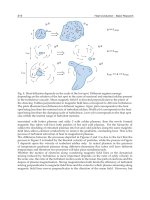
reciprocity BEM, the fundamental solution of lower order is used. The triple-reciprocity BEM
requires internal points similarly to the dual reciprocity method (DRM) (Partridge, 1992) as
shown in Fig. 1, although the boundary values

f
W need not be given analytically.



(a) Internal cells (b) Internal points
Fig. 1. Triple-reciprocity BEM.
2.2 Interpolation of heat generation
The distribution of heat generation W is interpolated using integral equations to transform the
domain integral into the boundary integral. The deformation of a thin plate is utilized to
interpolate the distribution of the heat source
1
S
W , where superscript S indicates a surface
distribution. The following equations can be used for interpolation (Ochiai, 1995a-c, 1996a, b):

2
12
SS
WW, (9)

Heat Conduction – Basic Research

328

2
23
1
()
M

SP
m
m
WWq



, (10)
where
3
P
W is a Dirac-type function, which has a value at only one point. The term
2
S
W in
Eq. (9) corresponds to the sum of curvatures
22
1
/
S
Wx

 and
22
1
/
S
W
y


 . From Eqs. (9)
and (10), the following equation can be obtained:

4
13
1
()
M
SP
m
m
WWq



. (11)
This equation is the same type of equation as that for the deformation
1
S
w of a thin
plate with point load
P, which is

4
1
1
M
S
m
m

P
w
D



, (12)
where the Poisson’s ratio is

=0 and the flexural rigidity is D=1. A natural spline originates
from the deformation of a thin beam, which is used to interpolate the one-dimensional
distribution, as shown in Fig. 2. In this chapter, the deformation of a thin plate is utilized to
interpolate the two-dimensional distribution
1
S
W . The deformation
1
S
w is given, and the force
of point load
P is unknown and is obtained inversely from the deformation of the fictitious
thin plate, as shown in Fig. 3. The term
2
S
W corresponds to the moment of the beam.


Fig. 2. Interpolation using thin beam with unknown point load.

Meshless Heat Conduction Analysis by Triple-Reciprocity Boundary Element Method

329

(a) Given internal points and boundary


(b) Obtained shape
1
S
W (c) Sum of curvatures
2
S
W
Fig. 3. Interpolation using fictitious thin plate with unknown point load.
The moment
2
S
W on the boundary is assumed to be 0, the same as in the case of the natural
spline. This means that the thin plate is simply supported. In this method, the distribution of
heat generation is assumed to be that for a freeform surface (Ochiai, 1995c). Equations (9)
and (10) are similar to the equation used to generate a freeform surface using integral
equations.
2.3 Representation of heat generation by integral equations
The distribution of heat generation is represented by an integral equation. The following
harmonic function
1
(,)Tpq and biharmonic function
2
(,)Tpq are used for interpolation
(Ochiai, 1999-2003).

1
11
(,) [ln() ]
2
Tpq B
r



(13)

2
2
1
(,) [ln() 1]
8
r
Tpq B
r


 (14)
B is an arbitrary constant.
1
(,)Tpq and
2
(,)Tpq have the relationship

2

21
(,) (,)T
pq
T
pq
. (15)

Heat Conduction – Basic Research

330
Let the number of
3
P
W be M. The heat generation
1
S
W is given by Green’s theorem and Eqs.
(9), (10) and (15) as

11
11 23
1
2
1
23
1 1
() (,)
() { (,) ()} () (,) ( )
() (,)
(1) ( , ) ( ) ( , ) ( ),

S
M
SSP
fm
m
S
M
ff
f
SP
ffmm
f m
WQ TPQ
cW P T P Q W Q d Q T P q W q
nn
WQ TPQ
TPQ WQ d TPq W q
nn




 






  









(16)
where 0.5c  on the smooth boundary and 1c

in the domain. Moreover,
2
S
W in Eq. (10)
is similarly given by

21
21 2
() (,)
() (,) ()
S
SS
WQ TPQ
cW P T P Q W Q d
nn
















13
1
(, ) ( )
M
P
mm
m
TPq W q



. (17)
The integral equations (16) and (17) are used to interpolate the distribution. The thin plate
spline F(p, q) used to make a freeform surface is defined as (Dyn, 1987, Micchelli, 1986)
F(p,q)=r
2
ln(r). (18)
Equations (14) and (18) include the same type of function. Assuming
1

() 0
S
WQ

, the values
of
3
P
W
and /
S
f
Wnare obtained using Eqs. (16) and (17).
2.4 Polyharmonic functions
The polyharmonic function ( , )
f
T
pq
is defined by

2
1
ff
TT


 . (19)
Therefore, ( , )
f
T

pq
for the Kth dimensional case can be obtained using the next equation

1
1
1
1
[]
K
ff
K
TrTdrdr
r





. (20)
From Eq. (20), ( , )
f
T
pq
for the two-dimensional case can be obtained using the next equation

1
1
[]
ff
TrTdrdr

r



. (21)
The function ( , )
f
T
pq
and its normal derivative for the two-dimensional case are explicitly
expressed as

2( 1)
2
1
(,) [ln()
2[(2 1)!!]
f
f
r
T
pq
B
r
f






1
1
1
s
g
n( 1) ]
f
e
f
e




, (22)

Meshless Heat Conduction Analysis by Triple-Reciprocity Boundary Element Method

331

23
2
(,)
1
[2( 1){ln( ) }
2 [(2 2)!!]
f
f
Tpq
r

f
B
nr
f







1
1
1
12( 1) ]
f
e
r
f
en



 


, (23)
where
(2 1)!! (2 1)(2 3)(2 5) 1ffff   
，and sgn() is the sign function.

For the one-dimensional case,

21
1
(,)
2(2 1)!
f
f
r
Tpq
f



, (24)


22
,
1
2(2 2)!
f
f
Tpq
rr
n
f
n







. (25)
For the three-dimensional case,

23
(,)
4(2 2)!
f
f
r
Tpq
f




, (26)

24
(,)
(2 3)
4(2 2)!
f
f
Tpq
fr
r

nfn








. (27)
Equations (16) and (17) are similar to the equation used to generate a freeform surface using
integral equations (Ochiai, 1995c).
Using Green’s theorem three times and Eqs. (9), (10) and (19), Eq. (2) becomes
1
1
() (,)
() { (,) ()} ()
TQ T PQ
CT P T P Q T Q d Q
nn






1
1
2
()

{(,)
S
WQ
TPQ
n







2
1
(,)
()} ()
S
TPQ
WQdQ
n



12
21
(,) ()
S
TP
q
W

q
d







1
1
() (,)
{(,) ()} ()
TQ T PQ
TPQ TQd Q
nn






1
1
2
()
{(,)
S
WQ
TPQ

n







2
1
(,)
()} ()
S
TPQ
WQdQ
n



12
32
(,) ()
S
T PqW qd







1
1
() (,)
{(,) ()} ()
TQ T PQ
TPQ TQd Q
nn







2
1
1
1
()
(1) { (, )
S
f
f
f
f
WQ
TPQ
n











1
(,)
()} ()
f
S
f
TPQ
WQdQ
n




1
33
1
(, ) ( )
M
P
mm
m

TPq W q





(28)

Heat Conduction – Basic Research

332
2.5 Interpolation for 3D case
In the three-dimensional case, the following equations are used for smooth interpolation:

2
12
() ()
SS
W
q
W
q
, (29)

2
23
1
() ( )
M
SP

Am
m
Wq W q



, (30)
where the function
3
P
A
W

expresses the state of a uniformly distributed polyharmonic
function in a spherical region with radius A. Figure 4 shows the shape of the polyharmonic
functions; the biharmonic function T
2
is not smooth at 0r

. In the three-dimensional case,
smooth interpolation cannot be obtained solely by using the biharmonic function T
2
. To
obtain smooth interpolation, a polyharmonic function with volume distribution T
2A
is
introduced. The function
f
A
T

shown in Fig. 5 is defined as (Ochiai, 2005)




Fig. 4. Polyharmonic functions (T
f
, T
fA
)

2
2
00 0
(,) [ { (,) sin } ]
A
fA f
T
pq
T
pq
addda

 

 
, (31)
where
A


is a spherical region with radius A, and S is the surface of a spherical shell with
radius a. The function T
fA
can be easily obtained using the relationships
222
2cosrRa aR

 and sindr aR d



as shown in Fig. 5. Therefore,

sin
r
ddr
aR


. (32)

Meshless Heat Conduction Analysis by Triple-Reciprocity Boundary Element Method

333
This function is written using r instead of R, similarly to Eqs. (26) and (27), although the
function obtained from Eq. (31) is a function of R. The newly defined function
f
A
T can be

explicitly written as

22
1
(,) {(2 )( ) (2 )( ) }
2(2 1)!
ff
fA
Tpq fArrA fArrA
rf


rA (33)

22
1
(,) {(2 )( ) (2 )( ) }
2(2 1)!
ff
fA
Tpq fArAr fArAr
rf


rA

. (34)
In Fig. 5, A=1. The newly defined functions
f
A

T used in the chapter can be explicitly written
as

3
1
3
A
A
T
r
 r>A (35)

22
1
3
6
A
Ar
T

 rA

(36)

32
2
2
()
65
A

AA
Tr
r
 r>A (37)

422 4
2
10 15
120
A
rrAA
T


rA

(38)

34 22 4
3
(35 42 3 )
2520
A
Ar rA A
T
r


r>A (39)

642 24 6
3
21 105 35
5040
A
rrA rAA
T
  
 rA

. (40)
The heat generation
1
S
W is given by Green’s theorem and Eqs. (29)-(31) as

2
1
1
1
()
() (1) { (,)
S
f
f
S
f
f
WQ
cW P T P Q

n








23
1
(,)
()} () (, ) ( )
M
f
SP
fAmAm
m
TPQ
WQdQ T P
q
W
q
n





(41)

Moreover,
2
S
W in Eq. (30) is similarly given by

2
21
()
() { (,)
S
S
WQ
cW P T P Q
n





1
213
1
(,)
()} () (, ) ( )
M
SP
A
mAm
m
TPQ

WQdQ T PqW q
n





. (42)
Equations (41) and (42) are similar to the equation used to generate the freeform surface
using integral equations. Using Green’s theorem three times and Eqs. (29), (30) and (15), Eq.
(2) becomes

Heat Conduction – Basic Research

334

Fig. 5. Notations in three-dimensional problem
1
1
() (,)
() { (, ) ()} ()
TQ T PQ
cT P T P Q T Q d Q
nn






2
1
1
1
()
(1) { (, )
S
f
f
f
f
WQ
TPQ
n










1
(,)
()} ()
f
S

f
TPQ
WQdQ
n




1
33
1
(, ) ( )
M
P
A
mAm
m
TPqWq





(43)
In the same manner, a polyharmonic function with surface distribution
f
B
T
is defined as
(Ochiai, 2009)

2
2
00
(,) ( (,) sin )
Bf f
Tpq TpqA dd





. (44)
The newly defined function
f
B
T
can be explicitly written as

21 21
{( ) ( ) }
(,)
2(2 1)!
ff
fB
Ar A r A
Tpq
fr





rA , (45)

21 21
{( ) ( ) }
(,)
2(2 1)!
ff
fB
AA r A r
Tpq
fr




rA

. (46)
Additionally, the temperature gradient is given by differentiating Equation (28), and
expressed as:
()
i
TP
x


2
11

(,) () (, )
{()}()
ii
TPQ TQ TPQ
TQ d Q
xn xn



 


2
1
1
1
(,) ()
(1) {
S
ff
f
i
f
TPQWQ
xn











2
1
(,)
()} ()
f
S
f
i
TPQ
WQdQ
xn






Meshless Heat Conduction Analysis by Triple-Reciprocity Boundary Element Method

335

1
3
3
1

(, )
()
M
P
m
m
i
m
TPq
Wq
x







(47)
The function ( , ) /
f
i
Tpq x and its normal derivative for the two-dimensional case are
explicitly expressed as

23
2
(,)
1
[2( 1){ln( ) }

2 [(2 2)!!]
f
f
i
Tpq
r
f
B
xr
f







1
1
1
12( 1) ]
f
i
e
r
f
ex




 


, (48)
2
24
2
(,)
1
{[ 2( 2) , , ][2( 1){ln( ) }
2 [(2 2)!!]
f
f
iiij
i
Tpq
r
nfrrnf B
xn r
f




  




1

1
1
1 2( 1) ] 2( 1) , , }
f
ii
j
e
f
frrn
e


   

(49)
2.6 Basic equations for unsteady heat conduction
In unsteady heat conduction problems with heat generation
1
(,)
S
Wqt, the temperature T is
obtained by solving

21
1
S
WT
T
t





 

, (50)
where κ and t are the thermal diffusivity and time, respectively. Denoting an arbitrary time
and the pseudo-initial temperature by

and
0
(,0)Tq , respectively, the boundary integral
equation for the temperature in the case of unsteady heat conduction is expressed as
(Wrobel, 2002)
*
1
0
(, ,,)
(,) [(,)
t
TPQt
cTPt TQ
n








*
1
(,)
(, ,,)]
TPQ
TPQt dd
n








*0
1
( , , ,0) ( ,0)TPqt Tq d



*
11
0
(,,,) (,)
t
S
TPqt W q dd









, (51)
where c=0.5 on the smooth boundary and c=1 in the domain. The notations Γ and Ω
represent the boundary and domain, respectively. The notations p and q become P and Q on
the boundary. In the case of K-dimensional problems, the time-dependent fundamental
solution
*
1
(,,,)Tpqt

in Eq. (51) used for the unsteady temperature analyses and its normal
derivative are given by

*
1
/2
1
(,,,) exp( )
4( )
K
Tpqt a
t

 




, (52)

Heat Conduction – Basic Research

336

*
1
2/21
(,,,)
exp( )
8( )
K
Tpqt
rr
a
nn
t

 







, (53)

where

2
4( )
r
a
t




. (54)
Here, r is the distance between the observation point p and the loading point q. As shown in
Eq. (51), when an arbitrary pseudo-initial temperature distribution
0
(,0)Tq exists in the
domain, a domain integral is necessary. Therefore, the triple-reciprocity BEM (Ochiai, 2001)
is used to avoid internal cells.
This study reveals that the problem of unsteady heat conduction with many time steps can
be solved effectively by the triple-reciprocity BEM. Two different numerical procedures can
be employed for the numerical solution of Eq. (51). One method requires internal cells. At
the end of each time step, the temperature at a sufficient number of internal points must be
computed for use as the initial temperature in the next time step. The other method uses the
history of boundary values, making internal cells unnecessary, if the initial temperature can
be assumed to be 0. However, the CPU time required for calculation increases rapidly with
increasing number of time steps. In the presented method, the temperature distributions in
some time steps are assumed to be pseudo-initial and are interpolated using integral
equations and internal points.
2.7 Interpolation of time-dependent value
Heat generation

1
(,)
S
Wqt is assumed to vary within each time step in accordance with the
time interpolation function such that

SS
Wqt
11
(,) W ψ , (55)
where
ψ is the time interpolation function. Let us now assume a linear variation of
1
(,)
S
Wqt,

1
f
f
tt
t




,
1
2
f

f
tt
t





, (56)
where
1
fff
ttt

  .
The following equations can be used to obtain time-dependent values of heat
generation
1
(, )
f
W
q
t :

2
12
(, ) (, )
SS
ff
W

q
tW
q
t, (57)

2
23
1
(, ) ( , )
M
SP
f
m
f
m
Wqt Wqt



. (58)

Meshless Heat Conduction Analysis by Triple-Reciprocity Boundary Element Method

337
An interpolation method for the pseudo-initial temperature distribution using the boundary
integral equations that avoids the use of internal cells is next shown. The pseudo-initial
temperature
0
(,0)T
q

in Eq. (51) is represented as
0
(,0)
S
T
q
.
The following equations can be used for the two-dimensional interpolation (Ochiai, 2001):

20 0
12
(,0) (,0)
SS
Tq Tq
, (59)

20 0
23
1
(,0) ( ,0)
M
SP
m
m
Tq Tq



. (60)
The term

0
2
S
T in Eq. (59) corresponds to the sum of the curvatures
20 2
1
/
S
Tx


and
20 2
1
/
S
T
y
. The term
S
T
0
2
is the unknown strength of a Dirac-type function. From Eqs. (59)
and (60), the following equation can be obtained.

40 0
13
1
(,0) (,0)

M
SP
m
Tq Tq



(61)
In this study, the deformation of an imaginary thin plate is utilized to interpolate the two-
dimensional distribution
0
1
S
T . The deformation
0
1
S
T is given, but the force of the point load
0
3
P
T
is unknown.
0
3
P
T
is obtained inversely from the deformation
0
1

S
T
of the fictitious thin
plate, as shown in Fig. 3.
0
2
S
T
corresponds to the moment of the thin plate. The moment
S
T
0
2
on the boundary is assumed to be 0, which is the same as that in the natural spline.
This indicates that the fictitious thin plate is simply supported.
Using Green’s second identity and Eqs. (59), (60) and (15), we obtain (Ochiai, 2001)
0
2
1
0
1
1
(,0)
(,0) (1) { (,)
S
f
f
S
f
f

TQ
cT P T P Q
n










00
23
1
(,)
(,0)} (, ) ( ,0)
M
f
SP
fmm
m
TPQ
TQ d TPqT q
n






, (62)
where M is the number of
0
3
P
T
. Moreover,
0
2
S
T
in Eq. (60) is similarly given by

0
0
2
21
(,0)
(,0) { (,)
S
S
TQ
cT P T P Q
n






00
1
213
1
(, )
(,0)} (, ) ( ,0)
M
SP
mm
m
TPQ
TQ d TPqTq
n





. (63)
The integral equations (62) and (63) are used to interpolate the pseudo-initial temperature
distribution
0
1
S
T . On the other hand, the polyharmonic function
*
(,,,)
f
T
pq

t

in the unsteady
heat conduction problem is defined by

Heat Conduction – Basic Research

338

2* *
1
(,,,) (,,,)
ff
T
pq
tT
pq
t



. (64)
Using Green’s theorem twice and Eqs. (54)- (57) and (61), Eq. (51) becomes
0
3
P
T
**
1
1

(,,,) (,,,)
ff
Tpqt rTpqtdrdr
r









2
*
1
0
1
(,)
(1) [ (, ,,)
S
t
f
f
f
f
WQ
TPQt
n













*
1
(, ,,)
(,)]
f
S
f
TPQt
WQ dd
n









*
3( ) 3
0
1
(,) ( ,,,)
M
t
PA
m
m
WqTPqtd








0
2
*
1
1
(,0)
(1) [ (, ,,0)
S
f
f
f

f
TQ
TPQt
n










*
1
0
(, ,,0)
(,0)]
f
S
f
TPQt
TQ d
n






0*
33
1
( ,0) ( , , ,0)
M
P
mm
m
Tq TPqt



. (65)
Therefore, it is clear that temperature analysis without the use of a domain integral is
possible, provided that the initial temperature
0
1
T
is interpolated using Eqs. (62) and (63). In
practice,
0
1
S
T and
2
/
S
Tn

 are obtained using results from the previous time step; however,

0
2
S
T ,
2
/
S
Tn and
0
3
P
T in Eq. (65) are not obtained in this way.
2.8 Polyharmonic function for unsteady state
The two-dimensional polyharmonic function
*
(,,,)
f
T
pq
t

in Eq. (65) is determined as

**
1
1
(,,,) (,,,)
ff
Tpqt rTpqtdrdr
r









. (66)
*
(,,,)
f
T
pq
t

in the unsteady state and its normal derivative are concretely given by


*
21
1
(,,,) () ln()
4
Tpqt Ea a C




, (67)


*
2
(,,,)
1
1exp( )
2
Tpqt
r
a
nrn







, (68)


2
*
31
(,,,) () ln()
16
r
T
pq

tEaaC




1
1 exp( ) () ln()
2]
aEa aC
aa
  


, (69)


*
3
1
(,,,)
() ln() 1
8
Tpqt
rr
Ea a C
nn








1exp( )
]
a
a


, (70)
where E
１(

) is the exponential integral function and C is Euler’s constant.