Advances in Mechatronics Part 4 pot

Artificial Intelligent Based Friction Modelling and Compensation in Motion Control System

49
1s
g
n( )
c
dF F
dx F


  



(9)
where
F is the friction as a function of displacement x ,
c
F is the Coulomb friction, 

is the
motion velocity and

is empirical parameter which determines the shapes of the model.
It is position dependent model which captures the hysteresis behavior of friction but fails to
account for stiction and Stribeck.
Another dynamic model was proposed and implemented by Canudas de Wit et al. (1995). In
addition, Canudas de wit et al. (1995) modified the Dahl model to incorporate breakaway
(stiction) friction and its dynamics together with Stribeck effect using exponential GFK to

give what is been referred to as Lugre friction. This model captures most of the
experimentally observed friction characteristics, and is the first dynamic model that seeks to
effect smooth transition between the two friction regimes without recourse to switching
function. It is mathematically given by

,
()
o
dz
z
dt g






(10)

1
() ()
to
dz
Fz F
dt


  



(11)
where
z
is average of bristle deflection,
t
F is the tangential friction force, ( )
g


is stribeck
friction for steady-state velocities,
F


is viscous friction coefficient, while
o

and
1
 are
dynamic parameters, which are respectively the frictional stiffness and frictional damping.
Lugre model has been employed for friction analysis and compensation in various control
systems (Wen-Fang, 2007).
However, Lugre model fails to capture the non-local memory effect of hysteresis. Leuven
model proposed by Swevers et. al., (2000) is an elaborate model than Lugre as it
incorporating hysteresis function with non-local memory behavior in pre-sliding regime.
Apart from its complexity that has rendered it less effective in control system application,
Lampaert et. al., (2002) pointed out two major problems associated with Leuven model
namely: discontinuity and memory stack algorithm.
GMS is a qualitative new formulation by Lampaert et.al. (2003) based on the rate-state

approach of the Lugre and the Leuven models. It is noteworthy that despite the unique
advantages of dynamic models, one of the major challenges associated with their practical
implementation is the dependency of the models on unmmeasurable internal state of the
system and/or availability of very high resolution of (order
6
10

) sensing devices
(Armstrong, 1991). Hence, many of the reported works employing complex dynamic friction
model are based on simulation study.
2.2 Non-parametric based techniques
Due to the complexity and difficulty associated with physical models of friction in terms of
model selection, parameters estimation, and implementation, non-parametric based
approach using Artificial Intelligent (AI) approach is been alternatively employed in control
systems for friction identification and compensation. Neural network (NN), fuzzy logic

Advances in Mechatronics

50
(FL)/adaptive neuro-fuzzy inference system (ANFIS), support vector machine (SVM), and
genetic algorithm are among the common AI methods that have been reportedly used in
positioning control system.
The theory of artificial neural network (ANN) is based on simulated nerve cells or neuron
which are joined together in a variety of ways to form network. The main feature of the
ANN is that it has the ability to learn effectively from the data, and has been identified as a
universal function approximator (Haykin, 1999). ANN with back propagation was proposed
by (Kemal M. Ciliza and Masaypshi Tomizukab, 2007; Wahyudi and Tijani, 2008) for friction
modeling and compensation with varying structures and applications. The performance of
classical friction model was compared with Multilayer Feedforward Network (MFN)-based
friction model for friction compensation in (Wahyudi and Tijani, 2008), and MFN was

reported to outperform the classical friction model. A hybrid ANN was developed by Kemal
and Masayoshi (2007) where static and adaptive parametric models are combined with
ANN to better capture the discontinuities at the zero velocity. A radial basis function (RBF)
approach was proposed in (Du and Nair, 1999; and Haung et al., 2000) where the center
points and variances of the Gaussian functions had to be chosen a priori. Gan and Danai
(2000) developed model-based neural network (MBNN), and structured according to
linearized state space model of the plant and incorporated into Lugre friction model in a
Linear Motor stage.
Despite the extensive use of ANN for friction modelling, no ANN structure has been agreed
upon for optimal friction modeling for a varieties of motion control systems. There is need
to extend the notion of MBNN for other friction models that are suitable for some motion
control systems. Some of the challenges associated with the use of ANN in friction modeling
include: selection of appropriate structures (layers, neurons, and models) for a particular
application, generalization and local minimal problems.
Though ANFIS has been applied in nonlinear system modeling and control (Stefan, 2000),
its application in friction modeling and compensation in motion control has not received
much attention in the literatures. ANFIS is a Tagaki Sugeno (TSK) based fuzzy inference
system implemented in the framework of adaptive networks (Jang 1995). It has the ability to
construct an input-output mapping based on both human knowledge (in the form of fuzzy
if-then rules) and stipulated input-output data pairs. Existing work related to the use of
Neuro-Fuzzy can be found in many areas such as velocity control in (Jun and Pyeong, 2000),
(Chorng-Shyan 2003). In the latter case, fuzzy inference system was introduced to
compensate for friction parameter variations. Recently Tijani et.al (2011) reported the
application of ANFIS in friction modelling and compensation in motion control system.
Their results confirmed that this technique produces better performance in friction
modelling than paramteric methods.
Application of Support Vector Regression (SVR) in adaptive friction compensation was
recently proposed (Wang et al., 2007, Ismaila et.al. 2009(b)). It is noted that SVR has not been
extensively explored as compared to ANN for friction modelling. Also, other forms of SVR
such as least square support vector regression regression (LS-SVR) has been proposed as

alternative to SVR with a more simplified optimization algorithm (Johan, Van Gestel, De
Brabanter and Vandewalle, 2002), however it is yet to be employed in friction identification.
In addition, GA was employed for the estimation of optimal parameters for Lugre
parametric models by De-peng (2005), while hybrid of ANN and Gafor friction modelling
has been reported in (Sung-Kwun et al., 2006).

Artificial Intelligent Based Friction Modelling and Compensation in Motion Control System

51
3. System modelling and identification
Development of an appropriate mathematical model is the first step in order to characterize
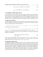
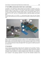
friction associated with motion control system. Figure 2 shows the experimental set-up of a
DC motor-driven rotary motion system which consists of servo motor driven by an
amplifier and position encoder attached to the shaft as the feedback sensor. The input to the
motor is the armature voltage
u
driven by a voltage source. The measurable variable is the
angular position of the shaft,

in radian, while the angular velocity of the motor shaft ( 

in
radian/s) is estimated using an appropriate digital filter. The plant was integrated into
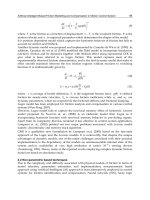
MATLAB xPC target environment as shown in Figure 3 for real-time experimental
implementation.
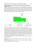
Basically, in line with model-based friction compensation approach, the system can be
decomposed into nominal (linear model) and non-linear sub-systems as shown in Figure4.
The nominal/linear sub-system is obtained from the physics of the system based on first
principle approach and system identication process for linear parameters estimation (Tijani
et.al,2009). The nonlinear sub-system on the other hand, represents the friction present in the

system. The friction occurs between various moving moving parts in the system. For
instance, it exists between the motor shaft and bearing, encoder shaft, external shaft, load
and associated bearing. As stated in section 2.1, the friction can take different form
depending on the geometary of the system and operating conditions. In this study, major
sliding friction effects dominating the sliding motion regime are considered. This consists of
stiction, Stribeck, and coulomb frcition as shown in Figure 2e. Note that the viscous friction
is regarded is included in linear sub-system model and its detailed derivation is reported in
(Tijani, 2009). The resulting second order mathematical model is given as

()
()
() ( 1)
p
sK
Gs
us s s




(12)
where 275K  and 0.1009
p


3.1 Friction identification experiments
Generally, in supervised AI-based modelling the availability of representative data is very
important. Two major experiments are required to obtain the velocity to friction relationship
for both break-away friction force and Stribeck friction. The major hardware, apart from the
Host and Target PC, are the National Instrument (NI) Multifunction input-output (I/O) data

acquisition (DAQ) PCI6024E, with BNC-2110 adapter for data acquisition to and from the
Target Pc. A Scancon incremental shaft encoder with resolution of
4
210x

(in quadrature
mode) was used for measuring the position in radian. A current sensor with 0-5Amp
current rating which is above the maximum current rating of the motor, 2Amp. was used
for measuring the armature current. A simple experiment based on Ohm’s Law was carried
out to test and model the V-I relationship of the sensor prior to the performance of the
experiment. This is required to transform the output voltage of the current sensor to
coresponding current.

Advances in Mechatronics

52




Fig. 2. DC-Motor driven rotary motion systems.


Fig. 3. MALAB xPC target set-up.


Fig. 4. Complete system model.
The resulting voltage-to-current relationship is given by

7.8555 19.6544

ss
IV
(13)
HOST
PC
DA
Q

TARGET
PC
PLANT
DRIVE


)(su
f

)( s


LINEAR MODEL
G(s)
FRICTION
MODEL

)( s


)( su
m

Servo drive
DC Motor
Load Encoder External shaft

Artificial Intelligent Based Friction Modelling and Compensation in Motion Control System

53
where
s
V is sensor output in volts and
s
I is equivalent current sensor output in amperes.
The first experiment tagged break-away experiment is to yield the break-away friction force
(
f
 ) in an open-loop mode. The break-away force is the force requires to initiate motion, in
other word it represents the stiction friction at zero velocity, i.e. the
0
()
f




. The
systematic steps followed according to (Armstrong, 1991) are:

“Warming-Up” of the Plant at beginning of each run


Gradual Increase of the motor Current at steps of 0.001volts command signal in pen
loop mode until the shaft moves (or breaks-away), this was taken to be at least 2
encoder counts.

Repetition of steps 1-2 for several times and Averaging of results in order to guarantee
repeatability
The procedures were repeated for both positive and negative directions of motion with 10
time runs for different days with a ramp input. The mean of the resulting values measured
by the current sensor in volts is then computed to give the average stiction friction force
2.531volt and 2.475volt for poistive and negative direction of motion respectively. The
difference between the friction force values in the poistive and negative directions of motion
justifies the asymetric nature of friction.
The second experiment involves identification of steady-state velocity-friction relationship.
The direct relationship between the friction torque,
f

and motor torque
m

at steady state
(i.e when
0

) is explored in this experiment. At steady state,
f
m

 , and since
m


is
proportional to the armature current
a
i
, it follows that
f

is propotional to
a
i
. The
experiement is conducted for a closed-loop system with an appropriate velocity controller.
Though any linear controller can be employed, a stiff velocity control scheme such as the
pseudo-derivative feedback with feedforward (PDFF) (Ohm,1990) has been shown to give
better performance especially at low-velocity control regime (Tijani, 2009). A suitable
velocity region is selected for both directions of motion to cover the low and high speed
above the region of Stribeck effect. For each constant velocity within this region, the average
of armature current and steady state velocity are then computed after the transient period of
0.2 second. Five different runs were carried out for each velocity input, and the overall mean
is computed. A total of 108 data sets were obtained for each direction of motion. Figure 5
and Figure 6 show samples of the steady state responses of the plant for positive and
negative directions respectively. Finally, the friction data aqcuired in voltage form based on
the output of the current sensor is transformed into actual armature current using the V-I
relationship in (13). The complete experimental data set for both directions are shown in
Figure 7.
4. Artificial intelligent based friction modelling and compensation
The development of Artificial Intelligent (AI) based friction modelling and application of
such model in friction compensation in motion control is described in this section. The
objective is to demonstrate the suitability of AI techniques in friction compensation in
motion control system. Though there exists several AI methods that can be applied based

on their approximating capability, the focus in this section is on the ANFIS and SVR based
on their unique characteristics over other AI methods.

Advances in Mechatronics

54
0.0 0.5 1.0 1.5 2.0 2.5
0.000
0.025
0.050
0.075
0.100
0.05 rad. input


Velocity (rad/s)
Time (sec.)
(a) 0.05- rad.
0.0 0.5 1.0 1.5 2.0 2.5
0.00
0.05
0.10
0.15
0.1 rad. input


Velocity (rad/s)
Time (sec.)
(b) 0.1-rad.
0.0 0.5 1.0 1.5 2.0 2.5

0.00
0.25
0.50
0.75
0.5 rad. input


Velocity (rad/s)
Time (sec.)
(c) 0.5-rad.
0.0 0.5 1.0 1.5 2.0 2.5
0.0
0.5
1.0
1.5
2.0
1 rad. input


Velocity (rad/s)
Time (sec.)
(d) 1-rad.
0.0 0.5 1.0 1.5 2.0 2.5
0
2
1.5rad. input


Velocity (rad/s)
Time (sec.)

(e) 1.5-rad.
0.0 0.5 1.0 1.5 2.0 2.5
0.0
0.5
1.0
1.5
2.0
2.5
3.0
2rad input


Velocity (rad/s)
Time (sec.)
(f) 2-rad.

Fig. 5. Samples of positive steady-state velocity responses.
0.0 0.5 1.0 1.5 2.0 2.5
-0.100
-0.075
-0.050
-0.025
0.000
-0.05 rad. input


Velocity (rad/s)
Time (sec.)
(a) -0.05-rad.
0.0 0.5 1.0 1.5 2.0 2.5

-0.15
-0.10
-0.05
0.00
-0.1 rad. input


Velocity (rad/s)
Time (sec.)
(b) -0.1-rad.
0.0 0.5 1.0 1.5 2.0 2.5
-0.75
-0.50
-0.25
0.00
-0.5 rad. input


Velocity (rad/s)
Time (sec.)
(c) -0.5-rad.
0.0 0.5 1.0 1.5 2.0 2.5
-2.0
-1.5
-1.0
-0.5
0.0
-1 rad. input

Velocity (rad/s)
Time (sec.)
(d) -1-rad.
0.0 0.5 1.0 1.5 2.0 2.5
-2.5
-2.0
-1.5
-1.0
-0.5
0.0
-1.5 rad. input


Velocity (rad/s)
Time (sec.)
(e) -1.5-rad.
0.0 0.5 1.0 1.5 2.0 2.5
-3.0
-2.5
-2.0
-1.5
-1.0
-0.5
0.0
-2 rad. input


Velocity (rad/s)
Time (sec.)
(f) -2-rad.

Fig. 6. Samples of negative steady-state velocity responses.

Artificial Intelligent Based Friction Modelling and Compensation in Motion Control System

55
-2.0 -1.5 -1.0 -0.5 0.0 0.5 1.0 1.5 2.0
-0.010
-0.005
0.000
0.005
0.010

Friction torque (Nm)
Velocity (rad/s)

Fig. 7. Complete experimental friction-velocity data set for both positive and negative
direction.
4.1 ANFIS and SVR as modeling tools
Both ANFIS and SVR are characterized with unique qualities that make them effective for
nonlinear system identification and modeling. ANFIS is an hybrid AI-paradigm, integrating
the best features of Fuzzy System (based on expert knowledge) and Neural Networks (based
on data mining) in solving the problems of transforming the expert knowledge into fuzzy
rules and tuning of membership functions associated with ordinary fuzzy inference system.
On the other hand, SVR is an extension of the well developed theories of Support vector
machine (SVM) to regression problems with introduction of

-insensitivity loss function by
Vapnik (1995). Unlike traditional learning algorithm for function estimation such as Neural
network that minimizes the error on the training data based on the principle of Empirical

risk minimization, SVR embodies the principle of structure risk minimization which
minimizes an upper bound on the expected risk. Hence, it is characterized by better ability
to generalize, and at the same time it is less prone to the problems of overfitting and local
minimal. Though initially developed for linear function estimation, the principle of linear
SVR was extended to non-linear case by the application of the kernel trick. Due to these
unique advantages, SVR has been recently employed for non-linear function approximation
and system modeling (Bi etal 2004, Ahmed etal 2008). A brief theoretical overview of the
two paradigms are given here while full detail can be obtained in the literatures (Jang, 1993,
Tijani et.al., 2011). It should be noted that there are two techniques of SVR namely
SVR and vSVR . The first is based on original concept of

-insensitivity Vapnik
(1995), and it involves the selection of appropriate

-parameter for the modelling process.
The challenges associated with the selection of

is overcome by the use of vSVR in

Advances in Mechatronics

56
which a parameter v is introduced to facilitate the optimal computation of  -sensitivity
function. Tijani (2009) reported a comparison of these two techniques. vSVR

was reporter
with both better modelling and compensation accuracy of friction in motion control system.
Hence, only the vSVR

is reported in this chapter while the reader is referred to the

literature for detailed review of the other two approaches
4.1.1 ANFIS overview
Basically, ANFIS implements Takagi Sugeno Fuzzy Inference System, and consists of five
layers minus the input layer O as shown in Figure 8. Besides the input layer O, each other
layer performs a specific function based on the associated node function as follows:
Layer 1 is responsible for the fuzzification of the input signal
1
X
and
2
X
with appropriate
membership function. It consists of adaptive nodes in which the parameters of membership
function are adjusted during learning process.
Layer 2 compute the firing strength
i

of each rule using a T-norm (min, product, etc) of the
incoming signals.
Layer 3 estimate the normalized firing strength,
i

of each fuzzy rule
Layer 4 also consists of adaptive nodes for computing the consequence parameters
i
Q
.
Layer 5 compute the overall output, O using a linear combination of all the incoming
signals from layer 4 :
Parametrically, ANFIS is represented by two parameter sets: the input/premise parameters

and the output/ consequence parameters.
4.1.2 SVR overview
Given a set of N input/output data
1
{,}
N
iii
xy

such that
n
i
x

 and
i
y


, the goal of
vSVR learning theory is to find a function
f
which minimizes the regularized risk
function(structural risk function) of the form (Sch¨olkopf and Smola, 2002):

2
1
[]: []
2
v

reg emp
RfRf wv


(14)


Fig. 8. Two inputs, one output typical ANFIS structure.

Artificial Intelligent Based Friction Modelling and Compensation in Motion Control System

57
where
2
1
2
w
is the regularization term(or complexity penalizer) used to find the flattest
function with sufficient approximation qualities,
[]
emp
R
f
is an empiric risk defined as:

1
1
[]: ( ,( ))
N
em

p
ii
i
Rf Lyfx
N



(15)
and parameter v is for automatic selection of optimal

and control of number of SVs. For
Vapnik’s
 -insensitivity, the loss function is defined as :

0()
() ()
()
if y f x
Ly y fx
yf
x otherwise






 





(16)
Methodologically, vSVR

processes are similar to that of SVR

 . It involves formulation
of the problem in the primal weight space as a constrained optimization problem by
formulating the Lagrangian, then take the conditions for optimality, and finally solve the
problem in the dual space of Lagrange multipliers called support values. Though, initially
developed for linear function estimation, the principle of linear SVR was extended to non-
linear case by the application of the kernel trick. For non-linear regression in the primal
weight space the model is of the form

() ()
T
f
xxb

 
(17)
where for the given training set
1
{,}
N
iii
xy


,
():
h
n
n


is a mapping to a high dimensional
feature space by the application of the kernel trick which is defined as
(,) () ()
T
i
j
i
j
Kx x x x  (18)
The constraint optimization problem in the primal weight space is
,,,
1
1
min ( , , , ) . ( )
2
N
T
Pii
b
i
JCv






      




Subject to:
()
T
ii
yxb

   1,2 ,iN



()
T
ii
xby


 1,2 ,iN

and , 0


 ,0


 (19)
where ,
ii

are the slack variables for soft margin
By defining the Lagrangian and applying the conditions for optimality solution, one obtains
the following v-SVR dual optimization problem:

,
,1 1
1
max ( , ) ( )( ) ( , ) ( )
2
NN
Dii
jj
i
j
ii i
ij i
JKxxy


 



    


Advances in Mechatronics

58
Subject to:
1
()0
N
ii
i


 

,

0,
ii
C
N


 


1,2, iN

and ().
N

ii
i
Cv

 

(20)
Thus, the regression estimate is given by

1
() ( )( , )
N
ii ij
i
f
xKxxb



 

(21)
where ,
ii

 are the Lagrange multipliers which are the solution to the Quadratic
optimization problem, and b follows from the complementary Karush-Kuhn-Tucker(KKT)
conditions (Scholkolpf and Smola,2002).
From the foregoing review, it is clear that the choice of Kernel function and the optimization
parameters to be selected aprior play important roles in overall performance of the

regression process. As previously reported in (Sch¨olkopf and Smola, 2002), the range
01vhas been identified as effective range of parameter v for control of errors, thereby
simplifying the selection range of parameters combination as compared to

-SVR.
4.2 Development of ANFIS friction model
The ANFIS-GP model was developed using MATLAB Fuzzy logic toolbox. First the data
was partitioned into training (60) and validation (40) data sets, and based on prior
information about the friction characteristics, two membership functions were assigned to
the input while the value of the premise parameters were initially set to satisfy  -
completeness (Lee,1990) with 0.5

 . The training was carried out using Hybrid training
with 0.0001 error target and 100 epochs. Figure 9 shows the resulting model with Gaussian
membership function.
4.3 Development of vSVR

friction model
The SVR-model was developed with reference to the original Matlab toolbox codes by Canu
et al (2005). The overall procedures are as follows:

Partitioning of data into training and validation sets.

Selection of Kernel function: e.g. Gaussian kernel

Selection and tuning of the regression parameters:

-Kernel parameter ( 01v), and
C–Capacity control for optimum performance. Various combinations of these
parameters were employed and cross-validated with testing data for both directions of

motion.

Computation of the difference of the Lagrange multipliers ( )
ii


 , support vectors
(nsv), bias term, b and epsilon,

.

Computation of the SVR/decision functions.
The resulting SVR models with training data and associated support vectors (circled ‘star
data points’) are shown in Figure10 (a) and (b) for positive and negative directions
respectively.

Artificial Intelligent Based Friction Modelling and Compensation in Motion Control System

59
-2 -1.5 -1 -0.5 0 0.5 1 1.5 2
-0.01
-0.008
-0.006
-0.004
-0.002
0
0.002
0.004
0.006
0.008

0.01
Velocity(rad/s)
Friction Torque(Nm )


ANFIS model
ANFIS Model
Friction Data
Friction Data

Fig. 9. ANFIS friction model with Gaussian membership function.
4.4 Friction compensation
The developed AI-based friction models are used in model-based friction compensation as
shown in Figure 11. The linear PD controller using root-locus technique with nominal plant
plant model given in equation (12). The use of PD controller is to enable proper evaluation
of the friction model performance since the controller does not have an integral action that
has the effect of suppressing the friction effect. The real-time scheme is implemented with
the MATLAB xPc target. ANFIS is implemented with the inbuilt MATLAB Fuzzy-Simulink
block while the resulting model parameters (difference of Lagrange multipliers and bias) of
the v-SVR are integrated to an embedded Matlab function for online real-time friction
compensation. Referring to Figure 11, the control law with friction compensation is given as:

ˆ
cin
f
uu u

 (22)
Hence it can be seen that if
ˆ

() ()
ff
uu



and the modeling error is approximately equal
zero, the effect of friction force is effectively compensated and the position accuracy
improved.
Figure 12 (a) and (b) show the the comparison of the response of the plant with and without
both ANFIS and v-SVR friction compensators for 0.1 and
1 degree step inputs . The tracking
errors for 0.1 and 1 degree for 1Hz sine wave input are shown in Figure 13 (a) and (b).
These were repeated for 0.5 and 10 degrees step (both directions) and sine wave reference
input, and the overall results are reported in Table 2 (a), (b) and Table 3 for point-to-point
and tracking control respectively in terms of response time, steady state accuracy and root
mean square error(RMSE).

Advances in Mechatronics

60
0 0.5 1 1.5 2
0
0.002
0.004
0.006
0.008
0.01
Velocity(rad/s)
Friction(Nm)

Data points
Svr function
Support vectors
Upper Margin
Lower Margin

(a) Positive direction.
-2 -1.5 -1 -0.5 0
-0.01
-0.008
-0.006
-0.004
-0.002
0
Velocity(rad/s)
Friction(Nm)


Data Points
Svr Function
Support Vectors
Upper Margin
Lower Magin

(b) Negative direction.
Fig. 10. SVRv  friction mod

Fig. 11. Control scheme for the model-based friction compensation.
PD
Controller



d


e

in
u

ref


f
u
ˆ

ref


c
u


ˆ


r


Velocity
Estimator
FRICTION
MODEL
PLANT

Artificial Intelligent Based Friction Modelling and Compensation in Motion Control System

61
5. Performance comparison of the proposed AI-models
The performance comparison of the two proposed AI-based friction models is carried out in
terms of modeling accuracy, compensation efficiency, and computational time/complexity.
The modeling accuracy refers to the performance of the model on training and validation is
data. Table 4 gives the comparison of the two models RMSE for both directions of motion.
The percentage reduction in both steady state and tracking error for each ANFIS-based and
SVRv  compensators was computed so as to compare their compensation efficiency as
shown respectively in Figure 14(a) and (b) and Figure 15. Also, the computational time for
training and prediction based on the MATLAB resources was computed to examine the
complexity of each model as reported in Table 5 .
6. Discussions
The performance improvements recorded with each of the friction compensators over only
linear PD controller indicate the importance and requirements of friction compensation for
precision positioning control especially at low reference input where the effect of negative
friction is highly deteriorating. Comparatively, a better modeling accuracy and
compensation efficiency were generally obtained with SVRv


as reported in Table 4, and
shown in Figure 14 (a) and (b) and Figure 15. Significant reduction in positioning error over
the use of only linear controller was observed in particular up to 90% reduction in steady
state error and 60% reduction in root mean square error for PTP and tracking respectively
with the v-SVR based friction compensators as against 90% and 50% reduction respectively
with ANFIS model. On the other hand, with the MATLAB resources employed, ANFIS is
less computational intensive with average computational time of 110ms per training while
SVRv  takes 220ms per each iteration in modeling of friction as indicated in Table 5. It
should be noted that, many iterative steps are required in SVR development as compared to
ANFIS. However, ANFIS is noted to have lesser prediction response with slower time
response of 1.6ms as compared to SVRv

with approximately 0.5ms. This implies a
tradeoff between desired performance accuracy in favor of SVR and less computational
efforts for model development in favor of ANFIS.
The general performance of SVR over ANFIS can be attributed to the fact that SVR
algorithm minimizes an upper bound on the expected risk, that is, SVR not only minimizes
the error on the training data as in ANFIS modeling but it also minimizes model complexity.
So it was able to generalize better than ANFIS on the noisy real-time velocity data during
the compensation especially for tracking control.

0.00 0.01 0.02 0.03 0.04 0.05
0.00
0.02
0.04
0.06
0.08
0.10
0.12

Position (degree)
T im e (sec.)
PDOnly
ANFIS
SVR

Fig. 12(a). 0.1 deg.

Advances in Mechatronics

62
0.00 0.02 0.04 0.06 0.08 0.10
0.0
0.2
0.4
0.6
0.8
1.0

Position (degree)
T im e (sec.)
PD O nly
ANFIS
SV R

Fig. 12(b). 1.0 deg.
Fig. 12. Step input responses with and without the Friction compensator.

0.00 0.25 0.50 0.75 1.00
-0 .1 0

-0 .0 5
0.00
0.05
0.10
PD O nly
Tim e
(
sec.
)
Pos. error
-0 .1 0
-0 .0 5
0.00
0.05
0.10
ANFIS

Pos. error
-0 .1 0
-0 .0 5
0.00
0.05
0.10
vSV R

Pos. error

(a) 0.1-deg. Sine input.

0.00 0.25 0.50 0.75 1.00

-0 .1 5
-0 .1 0
-0 .0 5
0.00
0.05
0.10
0.15
PD O nly
T im e (s e c .)
Pos. error
-0 .1 5
-0 .1 0
-0 .0 5
0.00
0.05
0.10
0.15
ANFIS

Pos. error
-0 .1 5
-0 .1 0
-0 .0 5
0.00
0.05
0.10
0.15
vSV R

Pos. error

(b) 1-deg. Sine input.
Fig. 13(a) and (b). Position tracking error for sinusoidal reference signal.

Artificial Intelligent Based Friction Modelling and Compensation in Motion Control System

63

POSITIVE STEP INPUTS

0.1-deg. 0.5-deg. 1-deg. 10-deg.
Friction
Compensators
ess(%)

Tr(sec.)

ess(%)

Tr(sec.)

ess(%)

Tr(sec.)

ess(%) Tr(sec.)
No
Compensator
75 N/A 37.6 N/A 7.6 0.017 1.8 0.015
ANFIS 4 0.0084 0.8 0.009 0.4 0.015 0.3 0.014

v-SVR 4 0.008 0.8 0.01 0.4 0.015 0.1 0.014
Table 2(a). Performance comparison results for positive PTP positioning control.


NEGATIVE STEP INPUTS

-0.1-deg. -0.5-deg. -1-deg. -10-deg.
Friction
Compensators
ess(%) Tr(sec.) ess(%) Tr(sec.) ess(%) Tr(sec.) ess(%) Tr(sec.)
No Compensator 76 N/A 44.26 N/A 21 0.017 1.24 0.015
ANFIS 4 0.009 0.8 0.008 0.4 0.012 0.1 0.014
v-SVR 4 0.008 0.8 0.013 0.4 0.013 0.04 0.014
Table 2(b). Performance comparison results for negative PTP positioning control.

Friction Compensators
Root Mean Square Errors (RMSE)
0.1-deg. 0.5-deg 1-deg. 10-deg.
No Compensator 0.0355 0.0656 0.0874 0.0959
ANFIS 0.0165 0.0277 0.0380 0.0587
v-SVR 0.0132 0.0255 0.0390 0.0608
Table 3. Performance comparison results for tracking positioning control.

Training RMSE Prediction RMSE
ANFIS
Positive Direction 0.000458 0.000443
Negative Direction 0.000725 0.000744
v-SVR
Positive Direction 0.000408 0.000430
Negative Direction 0.000690 0.000727

Table 4. Performance comparison in terms of the modelling accuracy.

Training
Computational
time(ms)
Prediction
Computational
time(ms)
ANFIS
Positive Direction 108.581 1.605
Negative Direction 110.080 1.605
v-SVR
Positive Direction 209.692 0.493
Negative Direction 224.828 0.493
Table 5. Performance comparison in terms of computational time.

Advances in Mechatronics

64
0.1-deg. 0.5-deg. 1-deg. 10-deg.
0
20
40
60
80
100
120
140
% error reduction
P ositiv e step in p u ts (d eg ree)

ANFIS
vSV R


-0.1 -deg . -0 .5-deg . -1-d eg. -10-deg .
0
20
40
60
80
100
120
140

% error reduction
N egative step inputs (degree)
ANFIS
vSV R

Fig. 14(a) and (b). Comparison of the ANFIS and SVRv

models in terms of %reduction in
steady state error over only PD controller for step inputs
0.1-deg. 0.5-deg. 1-deg. 10-deg.
0
20
40
60
80
100

% error reduction
Tracking inputs (degree)
ANFIS
vSV R

Fig. 15. Comparison of the ANFIS and SVRv

Models in terms %reduction in tracking
error over Only PD controller for tracking control.
Figure 14(a)
Figure 14(b)

Artificial Intelligent Based Friction Modelling and Compensation in Motion Control System

65
7. Conclusion
The application of artificial intelligent based techniques in friction modeling and
compensation in motion control system has been presented in this chapter. The chapter
focuses on comparative study of the two developed AI-friction models which have been
carried out in terms of modeling accuracy, compensation efficiency, and computational
time. In comparison, SVRv

outperformes ANFIS both in representing and compensating
the frictional effects especially for tracking control at low velocity regime. The results show
v-SVR to be better in representing friction than ANFIS with smaller RMSE for both training
and prediction of friction. Though, both perform equally in PTP control, v-SVR
outperformed ANFIS in tracking control with 60% to 50% reduction in tracking error.
Computationally, ANFIS is better with smaller computational processes and time for
modeling than SVR, but appears to be poor in prediction than SVR.
It is noted from this study that the performance of the friction model is greatly affected by

the precision of the sensor employed. This has limited the minimum velocity that can be
controlled to 0.1 degree. Apart from sensor effect, extension of these techniques to
micro/nano scale positioning control will required the incorporation of dynamic friction
model in the AI-friction model development.
Also, the velocity estimation from the position sensor used introduced noise in the feedback
signal. This is responsible for non-smoothness in the tracking responses. This can be
avoided either with the use of better position sensor together with more sophisticated
velocity filter or by using separate sensor to measure the velocity directly.
8. References
Ahmed G. Abo-Khalil and Dong-Choon Lee, (2008). MPPT Control of Wind Generation
Systems Based on Estimated Wind Speed Using SVR,IEEE Transactions on Industrial
Elecetronics,Vol.55,no. 3,March 2008.
Amontons, G., (1699). On the resistance originating in machines, Proc. of the French
Royal Academy of Sciences. pp. 206-22.
Armstrong-Helouvry B., Dupont P. and De Wit C., (1994). A survey of models, analysis tools
and compensation method for the control of machines with friction, Automatica, Vol. 30,
No. 7 (1994) pp. 1083-1138.
Armstrong-Helouvry B.,(1992) Control of Machines with Friction, Boston, MA, Kluwer, 1991
Bi.D, Y.F.Li, T.S.Tso, and G.L.Wang, (2004), Friction modeling and Compensation for Haptic
display based on Support Vector Machine, IEEE Trans. Ind. Electron.,vol. 51, no. 2, pp.
491-500,Apr.2004
Cai L. and G. Song, (1993). A smooth robust nonlinear controller for robot manipulators with joint
stick-slip friction, in Proceedings of IEEE Int. Conference on Robotics and
Automation,Atlanta,1993, pp.449-454.
Canudas de Wit, K.J. Astrom and K. Braun,(1986). Adaptive friction compensation in DC motor
drives, Proceeding of IEEE International Conference on Robotics and Automation,
San Francisco, Vol. 3, pp. 1556-1561,1986.
Canudas de Wit, H. Olsson, K. J. Astrom, and P. Lischinsky,(1995). A New Model for Control
of Systems with Friction, IEEE Transactions on Automatic Control, vol. 40, no. 3, pp.
419-425, 1995

Advances in Mechatronics

66
Canu S., Y.Grangyalet , V. Guigue,and A. Rakotomamonjy, (2005). SVM and Kernel Methods
Matlab Toolbox. PerceptionSystemes et Information, INSA de Rouen, Rouen, France,
2005.
Charles M. Close, Dean H. Frederick, and Jonathan C. Newell, (2002). Modeling and analysis
of dynamic systems, John Wiley and Sons, Inc.
Chorng-Shyan Lin, (2003). Recurrent neuro-fuzzy modeling and fuzzy MD control for flexible
servomechanisms, Journal of Intelligent and Robotic Systems 38: 213–235, © 2003
Kluwer Academic Publishers, printed in the Netherlands.
Coulomb, C. A. (1785). Theorie des machines simples, enayant egard au frottemen de leurs parties,
et a la roideur dews cordages”. Mem. Math Phys., x, 161-342.
Da Vinci, L. (1519). The Notebooks, Dover, NY.
Dahl P., (1968). A solid friction model, Technical Report TOR-0158H3107–18I-1, the Aerospace
Corporation, El Segundo, CA.
De-Peng Liu, (2005). Research on Parameter Identification of Friction Model forServo Systems
Based on Genetic Algorithms, Proceedings of the 2005 Fourth International
Conference on Machine Learning and Cybernetics, Guangzhou.
Dupont P. and B. Armstrong-Helouvry, (1993). Compensation techniques for servo with friction,
Proceeding of American Control Conference, San Francisco, Vol. 2, pp. 1915-1919,
1993.
Ehrich, N. E., (1991). An investigation of control strategies for friction compensation. M.S. Thesis,
Dept. of Electrical Engineering, University of Maryland, MA.
Envangelos G., Papadopoulos and Georgios C. Chasparis,(2002). Analysis and model based
control of servomechanisms with friction, Proc. of the International Conference on
Intelligent Robots and Systems (IROS 2002),EPFL Lausanne, Switzerland.
Farid Al-Bender and Jan Swevers, (2008). Characterization of friction force dynamics, IEEE
Control Systems Magazine, vol. 28, no.6, pp. 64-81.

Hashimoto, M., K. Koreyeda, T. Shimono, H. Tanaka, Y. Kiyosawa and H.Hirabayashi,
(1992). Experimental study on torque control using harmonic drive built-in torque sensors,
Proc. Inter. Conf on Robotics and Automation, IEEE,Nice, pp. 2026-2031.
Haykin S. (1999), Neural networks: a comprehensive foundation, 2nd Ed., New Jersey,
Prentice Hall.
Jang J.S.R. (1993). ANFIS: Adaptive-Network-Based Fuzzy Inference System”, IEEE Trans.
Systems, Man, Cybernetics,23 (5/6):665-685, 1993.
Jang J.S.R and N. Gulley, Natick, MA ,(1995). “The Fuzzy Logic Toolbox for use with MATLAB”:
The MathWorks Inc., 1995
Johan A.K. Suykens, Van Gestel T., De Brabanter J., De Moor B., Vandewalle J., (2002). Least
squares support vector machines, River Edge, NJ: World Scientific.
Jun Oh Jang and Pyeong Gi Le,(2000). Neuro-fuzzy control for dc motor friction compensation,
Proceedings of the 39Ih IEEE Conference on Decision and Control Sydney,
Australia.
Ismaila B. Tijani, Wahyudi M. and Talib H.H., (2011). Adaptive Neuro-Fuzzy Inference System
(ANFIS) for Friction Modeling and Compensation in Motion Control Syste, International
Journal of Modeling and Simulation, Volume
31, No. 1,2011, ACTA PRESS.
Ismaila B. Tijani, Wahyudi M. and Talib H.H., (2009). A Non-Parametric Friction Model for
Accurate Positioning Control using v-Support Vector Regression (v-SVR), Proc. of the
2009 IEEE/ASME International Conference on Advanced Intelligent Mechatronics

Artificial Intelligent Based Friction Modelling and Compensation in Motion Control System

67
will be held on July 14-17, 2009 in Suntec International Convention and Exhibition
Center, Singapore.
Karnopp D, (1985). Computer simulation of slip-stick friction in mechanical dynamic systems,
Journal of Dynamic Systems, Measurement, and Control, 107H1I:100–103.
Kemal M. Cılıza, Masayoshi Tomizukab (2007), (2007). Friction modeling and compensation for

motion control using hybrid neural network models, ScienceDirect, Engineering
Applications of Artificial Intelligence 20 (2007) 898–911.
Lampaert V., Swevers J., and Al-Bender F.,(2002). Modification of the Leuven integrated friction
model structure, IEEE Transactions on Automatic Control, 47, 4, pp. 683-687.
Lampaert, V., F. Al-Bender and J. Swevers, (2003). A Generalized Maxwell-Slip friction model
appropriate for control purposes, Proc. of the 2003 Int. Conference on Physics
and Control, Saint-Petersbourg, Russia, 1170-1178.
Ljung, L. (1987). System Identification: Theory for the User, Prentice-Hall, Englewood Cliffs, NJ.
Lörinc Márton and Béla Lantos, (2007). Modeling, identification, and compensation of stick-slip
friction, IEEE Trans. on Industrial Electronics, vol. 54, no. 1.
Makkar C.,W.E.Dixon,W.G.Sawyer,and G.Hu, (2005). A New Continously Differentiable
Friction Model for Control Ssystems Design, Proceedings of the 2005 IEEE/ASME
International Conference on Advaanced Intelligent Mechatronics
Monterey,California,USA,24-26 July,2005.
Morin A.J. (1833). New friction experiments carried out at Metz in 1831–1833, In Proc. of the
French Royal Academy of Sciences, volume 4, pages 1–128.
Ohm D.Y., (1990). A PDFF Controller for Tracking and Regulation in Motion Control,
Proceedings of 18
th
Conference, Intelligent Motion,Philadelphia,1990
Oppelt W., (1976). A historical review of autopilot development, research, and theory in Germany,
Journal of Dynamic Systems, Measurements, and Control, pages 215–23.
Reynolds, O., (1886). On the theory of lubrication and its application to Mr. Beauchamp Tower's
experiments, including an experimental determination of the viscosity of olive oil, Phil.
Trans. Royal Soc., 177, 157-234.
Rong-Hwang Horng, Li-Ren Lin and An-Chen Lee, (2006). LuGre model-based neural network
friction compensator in a linear motor stage, International Journal of Precision
Engineering and Manufacturing vol. 7, no.2.
Sch¨olkopf, B. and Smola A. (2002). Learning with Kernels,MIT Press,Cambridge MA, 2002
Shen, C. N. and H. Wang, (1964). Nonlinear compensation of a second- and third-order system

with dry friction. IEEE Trans. on Applications and Industry,83(71), 128-136.
Smola A.J. and B.Scholkopf,(2001). A tutorial on Support vector Regression, NeuroCOLT
Technical Report NC-TR-98-030, 2001.
Southward S.S., C.J. Radcliffe, C.R.Mac-Cluer, (1991). Robust nonlinear stick-slip friction
compensation, J.Dyn. syst.,Meas. Control 113,pp. 639-644.
Stefan Brock, (2000). Application of ANFIS controller for two - mass – system, ESIT 2000, 14-15,
Aachen, Germany.
Sung-Kwun Oh, Witold Pedrycz, Wan-Su Kim, and Hyun-Ki Kim1, (2006). GA-based
polynomial neural networks architecture and its application to multi-variable software
process, Q. Yang and G. Webb (Eds.): PRICAI 2006, LNAI 4099, pp. 834 – 838, 2006.©
Springer-Verlag Berlin Heidelberg

Advances in Mechatronics

68
Swevers J., Al-Bender F., Ganseman C., and Prajogo T., (2000). An integrated friction model
structure with improved presliding behavior for accurate friction compensation, IEEE
Trans. on Automatic Control, 45, pp. 675-686.
Tjahjowidodo, T., Al-Bender, F. and Brussel, HV, (2004). Friction Identification and
Compensation in a DC Motor, International Journal of JSPE Vol. 32, No. 3, pp. 200-
206.
Tijani Ismaila B., (2009). Friction Identification and Compensation in Motion Control System using
ANFIS and SVM, Master Thesis, Mechatronics Engineering Department,
International Islamic University Malaysia, 2009.
Tustin A. (1947), The effects of Backlash and of Speed-Dependent Friction on the Stability of Closed-
Cycle Control Systems, IEEE Journal,vol. 94,part 2A,p.143-51.
Wahyudi, Sato K. and Shimokohbe A. (2005). Robustness evaluation of three friction
compensation methods for point-to-point (ptp) positioning systems, Robotics and
autonomous system, Elsevier, Vol. 52, Issues 2-3, pp. 247-256
Wahyudi, (2003). Friction Identification and Compensation for High Precision Motion Control

System - Part 1: Friction Identification”, Proc. of Industrial Electronics Seminar (IES),
2003.
Wahyudi and Ismaila B. Tijani, (2008). Friction Compensation for Motion Control System using
Multilayer Feedforward Network, Proceeding of the 5th International Symposium on
Mechatronics and its Applications (ISMA08), Amman, Jordan, May 27-29, 2008
Wen-Fang Xie, (2007). Sliding-Mode-observer-based adaptive control for servo actuator with
friction, IEEE Trans. On Industrial Electronics, vol. 54, no.
Vapnik V., (1995). The Nature of Statistical Learning Theory, Springer,New York,1995.
Yi Guo, Zhihua Qu, Yehuda Braiman, Zhenyu Zhang and Jacob Barhen, (2008). Nanontribology
and nanoscale friction, IEEE Control Systems Magazine,vol. 28,no.6, pp. 92-100.
Zhixiang Hou, Quntai Shen and Heqing Li, (2003). Nonlinear System Identification Based on
ANFIS, IEEE Int. Conf. Neural Networks & Signal Processing, Nanjing, China,
December 14-17, 2003.