Novel Applications of the UWB Technologies Part 13 ppt

Frequency Domain Skin Artifact Removal Method for Ultra-Wideband Breast Cancer Detection 11
Fig. 3. Antenna array and tumor configuration
5. Evaluation of the performance of the frequency domain skin removal in
comparison with other methods
The present section applies the frequency domain skin removal method described in section 4
in different scenarios and compares its performance with other methods. The focus in the first
part is more on details of applying the formulation provided in Section 4 on a simplified breast
model. The second part will apply the method in a more realistic scenario and compares the
results with the other methods.
5.1 Simplified Breast Model
As discussed in Section 4, the backscattered signal of a UWB pulse is the summation of some
harmonic terms. The number of these terms depend on the number of scattering points and
the multiple scattering effect. Each harmonic term consists of a complex exponential and a
coefficient. The argument of this complex exponential is the pole of the hypothetical system
mentioned in Section 4. By removing the poles corresponding to the skin reflection from the
frequency domain signal, all the skin related information will be removed from time domain.
The process is as follows.
The received signals are first converted into frequency domain using Fast Fourier Transform
(FFT) algorithm. The frequency domain signals are then processed to extract the model
parameters stated in the previous section. Among these parameters, a
i
s are directly related
to the amplitudes of each of the backscattered pulses. This can be explained as follows. In
Equation (13), a
i
is a complex coefficient which can be written as |a
i
|e
jθ
i
where θ

i
is the phase
of a
i
. Taking the inverse Fourier transform of Equation (13) yields
x
(t)=
N
∑
i=1
|a
i
|
2α
i
cos(θ
i
)
α
2
i
+(t −4πR
i
/c)
2
(30)
As seen in Equation (30),
|a
i
| is proportional to the amplitude of the pulse in the time domain.

However, the amplitude of the pulse backscattered from the tumor is much smaller than the
skin backscatter. Hence, a threshold could be defined to remove poles with dominant a
i
values
from the frequency response of the signal. Removing the poles over the stated threshold
ensures that only the poles corresponding to the skin will be removed from the signal. This
will remove the skin effect both in the early time and the late time responses as the elimination
in frequency domain will affect the whole time domain signal. Hence, the tumor reflection will
347
Frequency Domain Skin Artifact Removal Method for Ultra-Wideband Breast Cancer Detection
12 Will-be-set-by-IN-TECH
be preserved without the skin late time response interference in the signal. After removing
the skin related poles, the frequency domain signal is reconstructed using the mathematical
model (13) and then converted back into the time domain using the inverse-FFT algorithm.
Hence, the reconstructed signal will only contain contributions from the tumor and clutter.
Clutter will be rejected later using confocal imaging algorithm described in Section 1. We will
Ant. No. x y z Ant. No. x y z
1 35.71 0 35 13 -35.71 0 35
2 34.50 10.24 35 14 -34.50 -10.24 35
3 30.93 17.86 35 15 -30.93 -17.86 35
4 25.26 26.26 35 16 -25.26 -26.26 35
5 17.86 30.93 35 17 -17.86 -30.93 35
6 9.24 35.50 35 18 -9.24 -35.50 35
7 0 35.71 35 19 0 -35.71 35
8 -9.24 35.50 35 20 9.24 -35.50 35
9 -17.86 30.93 35 21 17.86 -30.93 35
10 -25.50 26.26 35 22 25.26 -26.26 35
11 -30.93 17.86 35 23 30.93 -17.86 35
12 -34.50 10.24 35 24 34.50 -10.24 35
Table 1. Antenna Arrangement

first describe the idea in detail using a simplified simulated breast model using SEMCAD X
(version 13) software package for an antenna array with 24 elements in a circular configuration
around the breast in order to show the ability of the method to remove the skin reflection from
the backscattered signal. The breast medium is modeled by a hemisphere with a radius of
50mm and thickness of 2mm as the skin layer. A spherical tumor with a radius of 2mm is
placed on the central axis of the hemisphere and at a height of 35mm from the center of the
hemisphere (x = 0mm, y = 0mm, z = 35mm). The model and the antenna locations are shown
in Figure 3 and Table 1 respectively. The relative permittivities of the skin and breast tissues
are set to the values given by (Fear et al., 2002) (
r
(ski n)=36, 
r
(tissue)=9). The dielectric
value assigned to the tumor is the measured dielectric value of the malignant tumor 
r
= 50
(Fear et al., 2002). Figure 4 shows the signal received in channel 1 and its spectrum. As the
0 0.5 1 1.5
x 10
−9
−0.015
−0.01
−0.005
0
0.005
0.01
0.015
Time(ns)
Voltage(v)
(a) Signal received in channel 1

2 4 6 8 10 12 14
x 10
9
−2
−1.5
−1
−0.5
0
0.5
1
1.5
2
Frequency(GHz)
Voltage(v)
(b) Frequency response of the signal received in
channel 1
Fig. 4. Signal received in channel 1 and its frequency response
348
Novel Applications of the UWB Technologies
Frequency Domain Skin Artifact Removal Method for Ultra-Wideband Breast Cancer Detection 13
skin reflects the largest energy among the reflectors in the breast medium, the high energy
dominant poles in the frequency domain will correspond to the skin backscatter. Hence a
threshold may be used to remove these dominant poles. The threshold is defined based on
the ratio of the backscattered energies of the skin to the tumor and is obtained as follows.
We fix the threshold value a little higher than the ratio of the largest possible peak tumor to
the skin response times the maximum reflection coefficient value a
i
. The maximum reflection
coefficient corresponds to the largest scatterer which is the skin surface. Hence, by removing
all the poles with a

i
values larger than this threshold from early time response we make sure
that only reflections larger than the tumor reflection is removed from the signal. Many factors
can affect the skin to tumor response ratio and more study is needed to consider all the factors
affecting this ratio and obtain an optimized threshold value. Here, to show the basic idea of
the current method, we consider three factors, tumor size, skin thickness and tumor location
to determine the highest possible ratio. To experimentally estimate the highest possible skin to
tumor response ratio, the tumor reflection is isolated from the other reflections by performing
two different simulations. One simulation is done without the tumor and the second one
is with the tumor. Subtracting the results of these simulations yields the tumor signature.
According to (Ulger et al., 2003) breast skin thickness varies in the range of 0.5-3.1mm; hence
two extreme cases (0.5 and 3.1mm) are simulated in the experiments. The tumor size is set
2mm and 5mm which is well within the range of the early breast cancer. Then the tumor
location is varied on the line connecting the center to the antenna location from the center of
the breast hemisphere to 5mm below the inner layer of the skin as the tumors so close to the
skin can be detected by examining the surface of the breast.
Tables 2 and 3 show the tumor to skin peak response ratio for the skin thickness of 0.5mm and
3.1mm respectively.
Location \ Tumor size 2mm 5mm
Center 9.04E-05 1.81E-04
Under The Skin 3.80E-03 5.20E-03
Table 2. Skin to Tumor Ratio (Skin Thickness: 0.5mm)
Location \ Tumor size 2mm 5mm
Center 7.72E-05 1.69E-04
Under The Skin 2.10E-03 4.00E-03
Table 3. Skin to Tumor Ratio (Skin Thickness: 3.1mm)
As expected, the tumor to skin response ratio increases as the tumor size increases. As seen
in the tables, the maximum ratio is obtained when the tumor radius is 5mm and is located
5mm below the skin, the highest tumor to skin response ratio is 0.0021, i.e. the skin reflection
is about 476 times stronger than the largest tumor reflection. Hence, by setting the threshold a

little larger than 0.21% of the largest reflection coefficient (a
max
) and removing all the poles
with a
i
values larger than this threshold from early time response we ensure that all the
reflections larger than the tumor reflection is removed from the signal. This would be true
in all other cases as we chose the largest possible tumor response to define the threshold.
Here, we chose 0.0025
× the largest reflection coefficient as the threshold value. The poles
extracted from the signal in channel 1 are shown in Table 4; Eliminated poles are indicated by
a’
∗
’.
349
Frequency Domain Skin Artifact Removal Method for Ultra-Wideband Breast Cancer Detection
14 Will-be-set-by-IN-TECH
−50 −40 −30 −20 −10 0 10 20 30 40 50
−50
−40
−30
−20
−10
0
10
20
30
40
50
Fig. 5. Confocal imaging of the breast after removing the skin reflection

Figure 6 shows the backscattered signal after removing the skin reflection. In the figure, solid
line represents the reconstructed signal super-imposed with the original signal represented by
the dotted line. As seen in the figure the skin backscatter is removed from the signal. Figure 7
0 0.2 0.4 0.6 0.8 1 1.2 1.4 1.6 1.8 2
x 10
−9
−5
−4
−3
−2
−1
0
1
2
3
4
5
x 10
−3
Time(ns)
Voltage(v)
Fig. 6. The dotted line shows the original signal and the solid line is the signal after skin
backscatter removal.
shows a larger view of the late time part of the response. As shown in the figure, the late time
part of the signal, where the tumor response exists, has not been affected significantly.
5.2 Comparison with the Averaging and Weighted Average Methods
In this section, the performance of the frequency domain method is compared with the
averaging (Li & Hagness, 2001) and weighted average filter (Bond et al., 2003). To make the
breast model more realistic, the mapping of the dielectric values inside the breast medium is
obtained from an MRI image of a real breast as shown in Figure 8. The clutter produced due

to the heterogeneity of the breast tissue has significant effect on the effectiveness of the skin
subtraction methods. In the averaging based methods, the averaged clutter from all other
350
Novel Applications of the UWB Technologies
Frequency Domain Skin Artifact Removal Method for Ultra-Wideband Breast Cancer Detection 15
1.5 1.55 1.6 1.65 1.7 1.75 1.8 1.85 1.9 1.95 2
x 10
−9
−4
−3
−2
−1
0
1
2
3
4
x 10
−4
Time(ns)
Voltage(v)
Fig. 7. The late time response of the reconstructed signal (line with dots) vs. the original
signal (solid)
Pole No. Reflection Coefficient Pole No. Reflection Coefficient
1 0.006030024 16 0.000576253
2 *0.330168871 17 0.000817322
3 *2.769236715 18 0.001800899
4 *8.978906551 19 0.003023339
5 *17.21322261 (MAX) 20 0.002570893
6 *16.81465757 21 0.000965909

7 *7.610199166 22 0.00044818
8 *1.504612836 23 0.000653675
9 *0.255119890 24 0.001118491
10 *0.052006092 25 0.000111348
11 0.005144400 26 0.00232989
12 0.005526546 27 0.000489255
13 0.004168027 28 0.010678232
14 0.001581127 29 0.022283477
15 0.001108609 30 0.022266937
Table 4. Reflection Coefficients(Eliminated poles are identified by *)
channels is added to each channel and makes the tumor detection even more difficult. As
seen in Figure 8, different dielectric constants of the breast internal regions appear as varying
intensities in the gray scale image. The scale for this mapping is given beneath the image.
Here, the regions with different dielectric values are approximated by spheres. The radius
of the sphere is chosen as the circumference of the region divided by 2π. The center of the
spheres are located at the same height and distance as the center of the corresponding region
from the center of the breast. Assume that the vertical axis in Figure 8 is z and the horizontal
axis is x in the Cartesian coordinates. In this configuration, y would have an inward direction
perpendicular to the xz plane. To make the model 3D, the angle φ
i
(between the position
vectors of i
th
sphere center and x axis) are chosen randomly in the interval [−π , π]. In this
experiment, the tumor coordinates are x=0, y=0, z=35 (mm). Figure 9 shows the model
obtained. The locations of the sphere centers are given in Table 5.
351
Frequency Domain Skin Artifact Removal Method for Ultra-Wideband Breast Cancer Detection
16 Will-be-set-by-IN-TECH
Fig. 8. 2D mapping of the dielectric values of the different regions of the breast

tissue(source:(Kosmas & Rappaport, 2005))
Fig. 9. 3D Model Constructed based on MRI image, shaded region shows the scanning area
Region x y z 
r
Region x y z 
r
A 0 0 17 5.3 E 16 10 4 4.8
B -25 0.9 22 5.2 F 11 -9 11 5
C -28 26 5 4.8 G -36 -25 5.5 5
D 4 27 7 4.8 H 27 4.7 22 5.2
Table 5. Dielectric region centers (mm)
In this model, the skin layer thickness is set as 2mm. The antenna placement, physical
parameters of the normal breast tissue and tumor are set as described in the previous section.
As for the clutter regions, dielectric values are obtained from the MRI image as stated above.
These values are given in Table 5.
The skin reflection is removed from the simulated backscattered signals using all three
methods: frequency domain approach, averaging and weighted average filter to compare
the performance of these methods. A 2D image of the breast is formed by applying confocal
imaging process on the processed signals. The resulting images from the three methods are
shown in Figure 10. Due to the symmetry of the tumor location to the antenna elements in the
array, the tumor response is totally eliminated from the image processed by averaging and
filtering methods. This is because, the tumor response will add coherently in the averaging
process (due to the symmetry) and hence will appear in the average signal. Hence, subtracting
the average removes the tumor backscatter as well as the skin backscatter. However, in
frequency domain approach, each signal is processed separately and no other data is added
352
Novel Applications of the UWB Technologies
Frequency Domain Skin Artifact Removal Method for Ultra-Wideband Breast Cancer Detection 17
−50 −40 −30 −20 −10 0 10 20 30 40 50
−50

−40
−30
−20
−10
0
10
20
30
40
50
(a) Averaging
−50 −40 −30 −20 −10 0 10 20 30 40 50
−50
−40
−30
−20
−10
0
10
20
30
40
50
(b) Weighted Average Filter
−50 −40 −30 −20 −10 0 10 20 30 40 50
−50
−40
−30
−20
−10

0
10
20
30
40
50
(c) Pole Removal
Fig. 10. Breast images using three skin subtraction methods: Averaging(a), Weighted
Average(b), Pole removal(c)
to or subtracted from the signal, the tumor signature remains intact. This is confirmed in
Figure 10. As seen in the figure, the tumor is detected at the central axis of the breast.
To compare the performance of the three methods in general case, the tumor is located in off
center coordinates (x = 35 , y = 0, z = 15). The other parameters of the model are the same as
the previous model.
Again, the skin reflection is removed using the three mentioned methods. The results are
shown in Figure 11.
As the figure reveals, all three methods have eliminated the skin effect and the tumor is
detected in the resulting image. To further evaluate the performance of the skin removal
methods, the peak Tumor to Clutter Ratio (TCR) for the three methods is compared in Table 6.
As seen in the table, the tumor to clutter ratio is the highest for frequency domain approach
Skin-Removal Method TCR
Pole-Removal 3.831
Weighted Average 2.082
Averaging 1.837
Table 6. Tumor to Clutter Ratio (TCR)
353
Frequency Domain Skin Artifact Removal Method for Ultra-Wideband Breast Cancer Detection
18 Will-be-set-by-IN-TECH
−50 −40 −30 −20 −10 0 10 20 30 40 50
−50

−40
−30
−20
−10
0
10
20
30
40
(a) Averaging
−50 −40 −30 −20 −10 0 10 20 30 40 50
−50
−40
−30
−20
−10
0
10
20
30
40
50
(b) Weighted Average Filter
−50 −40 −30 −20 −10 0 10 20 30 40 50
−50
−40
−30
−20
−10
0

10
20
30
40
50
(c) Pole Removal
Fig. 11. Tumor at: x = 35,y=0,z=15(mm), Averaging(a), Weighted Average(b), Pole
removal(c)
and is the lowest for simple averaging. This is expected since pole removal method processes
each signal individually unlike the other two methods which add clutter from other signals
and degrade the tumor reflection.
6. Conclusion
The high contrast in the dielectric value of the skin relative to the normal breast tissue and
air produces a strong backscatter in UWB breast cancer detection method. Such strong
backscatter can totally mask the tumor reflection and hence has to be removed from the
signal. Currently, two methods are used in practice to remove skin reflection. Both methods
exploit the similarity of the skin reflection in the signals collected by an array of antennas to
reconstruct and remove the skin reflection. Although these methods can significantly reduce
the skin contribution in the backscattered signal, they have some shortcomings. Both methods
use averaging to estimate the skin backscatter from the signals collected in different elements
of the antenna array. As a result, if the tumor is approximately equidistant to some of the
elements of the array, its reflection will suffer a high attenuation in the processed signals.
This will make the tumor detection very difficult or even impossible. Another problem of the
354
Novel Applications of the UWB Technologies
Frequency Domain Skin Artifact Removal Method for Ultra-Wideband Breast Cancer Detection 19
averaging based methods is that they add the averaged version of the noise and clutter from
all channels to each individual channel which makes the tumor detection even more difficult.
In addition, as the tumor reflection should not be included in the skin reflection estimation
process, these methods need to determine the early time part of the signal where only the skin

reflection exists. However, the location of the tumor in the signal is not known prior to the
detection process.
This work introduces a new approach in removing the skin reflection from the backscattered
signal in UWB breast cancer detection. In this approach, the backscattered signals are
analyzed in frequency domain to identify and remove the skin related information from
the frequency response. Based on Geometrical Theory of Diffraction (GTD), a mathematical
model is applied on the frequency response of the signal. Then, the terms corresponding to
the skin are removed from the model and the signal is reconstructed. Performance of this
method is compared with the other existing methods in Section 5. As shown in Section 5,
the frequency domain approach can detect the tumor even when it is equidistant to all the
elements of the array. Besides, no extra noise and clutter is added to the signal as each signal is
processed individually. Thus, the frequency domain approach shows higher tumor to clutter
ratio in comparison with the other two methods. However, more investigations is needed
to determine some parameters of the process such as the threshold used to remove the skin
related terms from the frequency response. To optimize parameters such as the number of the
antenna elements needed in the array, type of the antenna, pulse shape, etc. the method has
to be applied on more realistic scenarios similar to the human breast.
7. References
Bond, E., Li, X., Hagness, S. & Van Veen, B. (2003). Microwave imaging via space-time
beamforming for early detection of breast cancer, IEEE Transactions On Antennas and
Propagation 51(8): 1690–1705.
Cuomo, K., Piou, J. & Mayhan, J. (1999). Ultrawide-band coherent processing, IEEE Microwave
Magazine 47(6): 1094–1107.
Fear, E., Li, X., Hagness, S. & Stuchly, M. (2002). Confocal microwave imaging for breast cancer
detection: Localization of tumors in three dimensions, IEEE Transactions on Biomedical
Engineering 49: 812–821.
Fear, E. & Stuchly, M. (2000). Microwave detection of breast cancer, IEEE Transactions On
Microwave Theory And Techniques 48(11): 1854 – 1863.
Hagness, S., Taflove, A. & Bridges, J. (1998). Two dimensional FDTD analysis of a
pulsed microwave confocal system for breast cancer detection: Fixed-focus and

antenna-array sensors, IEEE Trans. Biomed. Eng. 45: 1470–1479.
Haykin, S. (1996). Adaptive Filter Theory, 3rd edn, Prentice-Hall.
J. Elwood and B. Cox and A. Richardson (1993). The effectiveness of breast cancer screening
by mammography in younger women, The Online journal of current clinical trials 32.
URL: />Keller, J. (1958). A geometrical theory of diffraction, Courant Institute of Mathematical Sciences,
New York University.
Kosmas, P. & Rappaport, C. (2005). Time reversal with the FDTD method for microwave
breast cancer detection, IEEE Transactions on microwave theory and techniques
53(7): 2317–2322.
355
Frequency Domain Skin Artifact Removal Method for Ultra-Wideband Breast Cancer Detection
20 Will-be-set-by-IN-TECH
Li, X. & Hagness, S. (2001). A confocal microwave imaging algorithm for breast cancer
detection, IEEE Microwave and Wireless Components Letters 11(3): 130–132.
Moore, T., Zuerndorfer, B. & Burt, E. (1997). Enhanced imagery using
spectral-estimation-based techniques, Lincoln Laboratory Journal 10(2): 171–186.
Naishadham, K. & Piou, J. (2004). A super-resolution method for extraction of modal
responses in wideband data, IEEE Antennas and Propagation Society International
Symposium 4: 4168–4171.
Naishadham, K. & Piou, J. (2005). State-space spectral estimation of characteristic
electromagnetic responses in wideband data, IEEE Antennas and Wireless Propagation
Letters 4: 406–409.
Piou, J. (2005). A state identification method for 1-d measurements with gaps, Proc. American
Institute of Aeronautics and Astronautics Guidance Navigation and Control Conf. .
American Cancer Society (ACS) (2007). What are the key statistics for breast cancer?
URL: />_statistics_for_breast_cancer_5.asp
Center for Disease Control and Prevention (CDC) (2007). Statistics.
URL: />Ulger, H., Erdogan, N., Kumanlioglu, S. & Unur, E. (2003). Effect of age, breast size,
menopausal and hormonal status on mammographic skin thickness, Skin Research
and Technology 9: 284–289.

Zhi, W. & Chin, F. (2006). Entropy-based time window for artifact removal in uwb imaging of
breast cancer detection, IEEE Signal Processing Letters 13(10): 585–588.
356
Novel Applications of the UWB Technologies
Part 5
Novel UWB Application in
Radars and Localization Systems

17
Full-Wave Modelling of Ground-Penetrating
Radars: Antenna Mutual Coupling
Phenomena and Sub-Surface
Scattering Processes
Diego Caratelli and Alexander Yarovoy
Delft University of Technology
The Netherlands
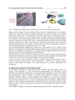
1. Introduction
Ground-penetrating radar (GPR) technology finds applications in many areas such as
geophysical prospecting, archaeology, civil engineering, environmental engineering, and
defence applications as a non-invasive sensing tool [3], [6], [18]. One key component in any
GPR system is the receiver/transmitter antenna. Desirable features for GPR antennas
include efficient radiation of ultra-wideband pulses into the ground, good impedance
matching over the operational frequency band, and small size. As the attenuation of radio
waves in geophysical media increases with frequency [9], [13], ground-penetrating radars
typically operate at frequencies below
1GHz [4]. For either impulse [13] or stepped-
frequency continuous-wave applications [17], the wider the frequency range, the better the
range resolution of the radar. Continuous wave multi-frequency radars are advantageous
over impulse radars in coping with dispersion of the medium, the noise level at the receiver
end, and the controllability of working frequency. They require, however, mutual coupling

between the transmit (Tx) and receive (Rx) antennas, which determines the dynamic range
of the system, to be kept as small as possible [12].
In this book chapter, the full-wave analysis of electromagnetic coupling mechanisms
between resistively loaded wideband dipole antennas operating in realistic GPR scenarios is
carried out. To this end, a locally conformal finite-difference time-domain (FDTD)
technique, useful to model electromagnetic structures having complex geometry, is adopted
[1], [2]. Such a scheme, necessary to improve the numerical accuracy of the conventional
FDTD algorithm [19], [21], by avoiding staircase approximation, is based on the definition of
effective material parameters [14], suitable to describe the geometrical and electrical
characteristics of the structure under analysis. By doing so, the losses in the soil, as well as
the presence of ground-embedded inhomogeneities with arbitrary shape and electrical
properties, are properly taken into account. Emphasis is devoted to the investigation of the
antenna pair performance for different Tx–Rx separations and elevations over the ground,
as well as on scattering from dielectric and metallic pipes buried at different depths and
having different geometrical and electrical characteristics. Novelty of the analysis lies in the

Novel Applications of the UWB Technologies

360
fact that at the lowest operational frequency both the receive antenna and a pipe are situated
in the near-field, whilst at the highest operational frequency only the far field is playing the
role. The obtained numerical results provide a physical insight into the underlying
mechanisms of subsurface diffraction and antenna mutual coupling processes. This
information in turn can be usefully employed to optimize the performance of detection
algorithms in terms of clutter rejection.
Finally, a frequency-independent equivalent circuit model of antenna pairs is provided in
order to facilitate the design of the RF front-end of ground-penetrating radars by means of
suitable software CAD tools. The procedure employed to extract the equivalent circuit is
based on a heuristic modification of the Cauer’s network synthesis technique [10] useful to
model ohmic and radiation losses. In this way, one can obtain a meaningful description of

the natural resonant modes describing the electromagnetic behaviour of antenna pairs for
GPR systems.
2. Locally conformal finite-difference time-domain technique
The analysis and design of complex radiating structures requires accurate electromagnetic
field prediction models. One such widely used technique is the FDTD algorithm. However,
in the conventional formulation proposed by Yee [19], [21], each cell of the computational
grid is implicitly supposed to be filled by a homogeneous material. For this reason, the
adoption of Cartesian meshes could result in reduced numerical accuracy when structures
having curved boundaries have to be modelled. In this case, locally conformal FDTD
schemes [1], [2] provide clear advantages over the use of the stair-casing approach or
unstructured and stretched space lattices, potentially suffering from significant numerical
dispersion and/or instability [19]. Such schemes, necessary to improve the numerical
accuracy of the conventional algorithm, are based on the definition of effective material
parameters suitable to describe the geometrical and electrical characteristics of the structure
under analysis.
In this section, a computationally enhanced formulation of the locally conformal FDTD
scheme proposed in [1] is described. To this end, let us consider a three-dimensional domain
D
filled by a linear, isotropic, non dispersive material, having permittivity
()

r
, magnetic
permeability
() r
, and electrical conductivity
() r
. In such a domain, a dual-space, non-
uniform lattice formed by a primary and secondary mesh is introduced. The primary mesh
D

M
is composed of space-filling hexahedrons, whose vertices are defined by the Cartesian
coordinates:



(,,)| 0,, ; 0,, ; 0,, .
ijk x y z
xyz i N j N k N 
(1)
As a consequence, the edge lengths between adjacent vertices in
D
M
result to be expressed
as:

1
1
1
,0,1,,1,
,0,1,,1,
,0,1,,1.
ii i x
jj j y
kk k z
xx x i N
yy y j N
zz z k N






  


  



  




(2)
Full-Wave Modelling of Ground-Penetrating Radars:
Antenna Mutual Coupling Phenomena and Sub-Surface Scattering Processes

361

The secondary or dual mesh
D
M

(see Fig. 1) is composed of the closed hexahedrons whose
edges penetrate the shared faces of the primary cells and connect the relevant centroids,
having coordinates
1/2
/2

iii
xxx


 ,
1/2
/2
jjj
yyy


 ,
1/2
/2
kkk
zzz


 . A set of
dual edge lengths is then introduced in
D
M

as follows:





1

1
1
/2, 1,2, , 1,
/2, 1,2, , 1,
/2, 1,2, , 1.
i
j
k
xii x
yjj y
zkk z
xx i N
yy j N
zz k N





  



  



  






(3)
As usual, the electric field components are defined along each edge of a primary lattice cell,
whereas the magnetic field components are assumed to be located along the edges of the
secondary lattice cells. In this formulation, the relationship between
E

and
H 
field
components is given by Maxwell’s equations expressed in integral form, specifically using
Faraday-Neumann’s law and Ampere’s law, respectively. In particular, the enforcement of
the Ampere’s law on the generic dual-mesh cell surface
1/2, ,
x
i
j
k
S


having boundary
1/2, , 1/2, ,
xx
i
j
ki
j

k
SC



(see Fig. 1) results in the following integral equation:


Fig. 1. Cross-sectional view of the FDTD computational grid in presence of curved
boundaries between different dielectric materials.

Novel Applications of the UWB Technologies

362

1/2, , 1/2, , 1/2, ,
(,) () (,) () (,) ,
xx x
ijk ijk ijk
xx
CS S
t E tdS E tdS
t
 

   

 
 


Hrdl rr rr (4)
where:











11 11
22 22
1/2, ,
11 11
22 22
,,,,,,,
,, , ,, ,
k
x
ijk
j jk
zz k z k
ij ij
C
yy j y j y z
ik ik
tHxyztHxyzt

Hx yz t Hx yz t o o

 
 

















Hr dl
(5)
as
j
y
 and
k
z
 tend to zero. Under the assumption that the spatial increments

i
x ,
j
y ,
k
z of the computational grid are small compared to the minimum working wavelength,
the infinitesimal terms of higher order appearing in (5) can be neglected. Furthermore, it
should be noticed that the
x

component of the electric field is continuous along the
interfaces crossing
1/2, ,
x
i
j
k
S


so that, under the mentioned hypothesis, the following
approximation can be made:



1
2
1/2, , 1/2, ,
() (,) , , , () .
x x

ijk ijk
xxjk
i
SS
EtdSExyzt dS
 


 
 

 
 

rr r (6)
Hence, combining the equations above yields:

11
11
22
22
11 11
11 11
22 22
22 22
,, ,,
,, ,,
,, ,,
,, ,,
() ()

() () () () ,
eff eff
xx xx
ijk ijk
ijk ijk
zzyy
ijk ijk
ijk ijk
tt
t
tttt


 
 






(7)
where we have introduced the normalized field quantities:



1
1
2
2

,,
() , , , ,
xixjk
i
ijk
txExyzt


 (8)



11
11
22
22
,,
() , , , ,
k
zzzk
ij
ijk
tHxyzt


  (9)



11

11
22
22
,,
() , , , ,
j
yyyj
ik
ijk
tHxyzt


  (10)
and the averaged effective permittivity
1/2, ,
eff
x
i
j
k
 , and conductivity
1/2, ,
eff
x
i
j
k
 , defined
as follows:



1/2
1/2
1
2
1
1/2 1/2
2
,,
1
,, .
j
k
kj
y
z
eff
i
i
x
zy
ijk
x y z dydz
x







 

 


 

(11)
Full-Wave Modelling of Ground-Penetrating Radars:
Antenna Mutual Coupling Phenomena and Sub-Surface Scattering Processes

363

The time derivative in (7) is then evaluated using a central-difference approximation that is
second order-accurate if
E

and H

field components are staggered in time domain [19].
This results in the following explicit time-stepping relation:


1
2
11
1
11
22

2
22
11
() ()
,, ,,
,,
,, ,,
,
n
nn
EE
xxxx
x
ijk ijk
i
j
k
ijk ijk





    (12)
where:


11
1
11

22
2
22
11 11
1
11 11
22 22
2
22 22
,, ,,
,,
,, ,,
nn
n
nn
zzyy
x
ijk ijk
ijk
i
j
ki
j
k



 




    
(13)
denotes the finite-difference expression of the normalized
x

component of the magnetic
field curl at the time step
1/2n  . In (12), the information regarding the local physical and
geometrical properties of the electromagnetic structure under analysis is transferred to the
position-dependent coefficients:

1
2
1
2
1
2
,,
()
,,
,,
1
,
1
eff
x
i
j
k

E
x
eff
ijk
x
i
j
k
Q
Q






(14)

1
2
1
2
1
2
,,
()
,,
,,
,
1

eff
x
i
j
k
E
x
eff
ijk
x
i
j
k
t
Q






(15)
with:

1
2
1
2
1
2

,,
,,
,,
.
2
eff
x
ijk
eff
x
eff
ijk
x
i
j
k
t
Q







(16)
The update equations of the remaining components of the electric and magnetic field can be
easily derived by permuting the spatial indices i ,
j
, k and applying the duality principle

in the discrete space.
As it can be readily noticed, the computation of position-dependent coefficients (14)-(16) can
be carried out before the FDTD-method time marching starts. As a consequence, unlike in
conformal techniques based on stretched space lattices, no additional correction is required
in the core of the numerical algorithm. Furthermore, the resulting FDTD update equations
(12)-(13) have a very convenient structure, leading to a 14% reduction of the number of
floating-point operations needed to determine the unknown field quantities in the generic
mesh cell compared to the Yee algorithm [19], [21]. It is also to be pointed out that the
proposed scheme has the same numerical stability properties as the conventional FDTD
formulation, although it introduces a significant improvement in accuracy over the stair-
casing approximation as well as alternative weighted averaging FDTD approaches [7]. In
order to assess the effectiveness of the developed technique, several test cases have been
considered. For the sake of brevity, only the computation of the fundamental resonant

Novel Applications of the UWB Technologies

364
frequency of a metallic cavity loaded with a cylindrical dielectric resonator is presented in
the Appendix. The obtained results clearly demonstrate the suitability of the proposed
scheme to efficiently handle the problem of modelling antennas for ground-penetrating
radar applications, where the accurate characterization of complex metal-dielectric objects
having irregular geometry (think about the shape of buried targets and ground-embedded
inhomogeneities) is required.
3. The full-wave antenna modelling
It is our intention to focus the attention on the full-wave analysis of a resistively loaded
dipole antenna pair located above a ground modelled as a lossy homogeneous half-space
having relative permittivity
6
r


 and electrical conductivity 15mS m

 . The geometry of
the structure is depicted in Fig. 2.


Fig. 2. Top and cross-sectional view of a resistively loaded dipole antenna pair located above
a lossy homogeneous half space. Structure characteristics:
40
d
lcm
,
5
d
Dmm
,
2.5mm
,
6
r

,
15mS m
. The reference system used to express the field quantities is
also shown.
The dipoles are denoted as dipole
#1
and dipole
#2
, respectively. In the considered

antenna configuration, dipole
#1
is driven by a delta-gap voltage source with internal
resistance
1
300
G
RR 
, whereas dipole
#2
is closed on a matched load having
resistance
2LG
RRR
. To properly enlarge the antenna bandwidth, thus reducing late-
time ringing phenomena, a continuous resistive loading, having Wu-King-like profile [3],
[15], [16]:
Full-Wave Modelling of Ground-Penetrating Radars:
Antenna Mutual Coupling Phenomena and Sub-Surface Scattering Processes

36
5


0
2
1,
d
d
y

y
l





(17)
has been applied to the flairs of the considered radiators. In (17),
0

denotes the electrical
conductivity value at the input terminals of the antennas (
0y

), and 40
d
lcm

is the
length of each dipole, assumed to have diameter
5
d
Dmm

. In particular,
0
 has been
determined by means of a dedicated parametric analysis. In this way, the optimal value
0

200 /
opt
Sm  , resulting in a fractional bandwidth 51%FBW  centred on the
fundamental resonant frequency
450
r
f
MHz , has been found (see Fig. 3).


Fig. 3. Frequency behaviour of the individual antenna input reflection coefficient for
different loading profiles. The antenna is elevated
3
d
hcm

over the ground.
The FDTD characterization of the structure has been carried out by using a non-uniform
computational grid with maximum cell size
min
24 2.5hmm

  , where
min
6cm

 is the
wavelength in the ground at the upper 10dB

cut-off frequency

max
1
f
GHz

of the
excitation voltage signal, which is the Gaussian voltage pulse described by the equation:

2
0
ˆ
() exp (),
GG
G
tT
vt V ut
T










(18)
where
ˆ

1
G
VmV ,
0
10
G
TT

, and:

max
ln10
0.48 .
G
Tns
f



(19)
In (18),
()ut denotes the usual Heaviside function. The source pulse is coupled into the
finite-difference equations used to update the time-domain electric field distribution within
the feed point of dipole
#1
as follows:

Novel Applications of the UWB Technologies

366


1
1
2
2
11
11
1
11 1 11 1
11 1 11 1
22
22
11 1
2
11
(,) (,)
,, ,,
,, ,,
,,
,
n
nn
n
EG EG
yy yy G
y
ij k ij k
ij k ij k
ij k









   




 
(20)
where:

1
11 1
2
1
11 1
2
1
11 1
2
(,)
,,
(,)
(,)

,,
,,
1
,
1
EG
y
ij k
EG
y
EG
ij k
y
ij k
Q
Q






(21)

1
11 1
2
1
11 1
2

1
11 1
2
,,
(,)
(,)
,,
,,
,
1
eff
y
ij k
EG
y
EG
ij k
y
i
j
k
t
Q






(22)

with:

1
11 1
2
1
11 1
2
(,)
,,
,,
,
2
EG
y
eff
ij k
y
G
ij k
t
Q
R





(23)
1

i
,
1
j
,
1
k
being the spatial indices relevant to the source. In (20), the term:

1
2
(1/2)
()
n
G
G
G
tn t
vt
R



 (24)
denotes the time-discretised nominal current delivered by the generator. Similarly, the
electric field distribution within the feed point of dipole
#2
is updated by using the finite-
difference equation:


1
2
11
11
1
22 2 22 2
22 2 22 2
22
22
22 2
2
11
(,) (,)
,, ,,
,, ,,
,,
,
n
nn
EL EL
yyyy
y
ij k ij k
ij k ij k
i
j
k






   
(25)
where:

1
22 2
2
1
22 2
2
1
22 2
2
(,)
,,
(,)
(,)
,,
,,
1
,
1
EL
y
ij k
EL
y

EL
ij k
y
ij k
Q
Q






(26)

1
22 2
2
1
22 2
2
1
22 2
2
,,
(,)
(,)
,,
,,
,
1

eff
y
ij k
EL
y
EL
ij k
y
ij k
t
Q






(27)

1
22 2
2
1
22 2
2
(,)
,,
,,
,
2

EL
y
eff
ij k
y
L
ij k
t
Q
R





(28)
Full-Wave Modelling of Ground-Penetrating Radars:
Antenna Mutual Coupling Phenomena and Sub-Surface Scattering Processes

36
7
and with
2
i ,
2
j ,
2
k denoting the spatial indices relevant to the load. The total voltage and
current signals excited at the input terminals of the antenna pair, regarded as a two-port
microwave network, are readily computed as:

1
2
,,
() (,) () ,
V
mm m
m
my
C
ij k
vt t t

  

Er dl 
(29)


1111
2222
11 11 11 11
22 22 22 22
,, ,, ,, ,,
() , ,
mmm mmm mmm mmm
I
m
nnnn
m xxzz

ij k ij k i j k i j k
C
it t

   
   



Hr dl 
(30)
where
m
V
C is an open contour extending along the delta gap, and
m
I
C a closed contour path
wrapping around the driving point of dipole #m (
1,2m

). Under the mentioned
assumptions, the normalized incident and reflected waves are evaluated as:

1
110
0
()
1
() () ,

2
Vf
af If R
R







(31)

1
110
0
()
1
() () ,
2
Vf
bf If R
R








(32)

2
() 0,af (33)

2
2
0
()
() ,
Vf
bf
R
 (34)
where
0 G
RR
denotes the reference resistance and


() ()
mm
Vf vt F ,


() ()
mm
If it F ,
[]F

being the usual Fourier transform operator. Therefore, the scattering parameters of the
structure can be easily determined as:

1
11
1
()
() ,
()
bf
Sf
af

(35)

2
21
1
()
() .
()
bf
Sf
af

(36)
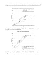
As it appears from Fig. 4a, the return-loss level is slightly affected by the Tx–Rx antenna
separation that, on the other hand, is primarily responsible for the parasitic coupling level
between the radiating elements. The impact of the antenna elevation above the ground has
been also analyzed (see Fig. 4b). It is worth noting that, as

d
h decreases, the fundamental
resonant frequency of the dipole is shifted down because of the proximity effect of the soil.
On the other hand, the ground influence on the
21
S parameter is remarkable only at high
frequencies, where the coupling level between the two radiating elements tends to decrease
as the dipoles approach the air-ground interface.
In the performed numerical computations, a ten-cell uniaxial perfectly matched layer (UPML)
absorbing boundary condition for lossy media [19] has been used at the outer FDTD mesh
boundary to simulate the extension of the space lattice to infinity. As outlined in [19], the

Novel Applications of the UWB Technologies

368
UPML is indeed perfectly matched to the inhomogeneous medium formed by the upper air
region and the lossy material modelling the soil. So, no spurious numerical reflections take
place at the air-ground interface. In particular, a quartic polynomial grading of the UPML
conductivity profile has been selected in order to have a nominal reflection error
16
PML
Re

 .


(a)


(b)

Fig. 4. Frequency behaviour of the scattering parameters of the dipole pair for different Tx–
Rx separations (a) and antenna elevations (b) over the ground modelled as a lossy
homogeneous half-space with electrical properties
6
r

 and 15mS m

 .
Full-Wave Modelling of Ground-Penetrating Radars:
Antenna Mutual Coupling Phenomena and Sub-Surface Scattering Processes

369

4. The radar detection of buried pipes
In this section, emphasis is devoted to the analysis of the dipole antenna pair located above
a lossy homogeneous/inhomogeneous material half space where an infinitely long pipe is
buried (see Fig. 5). In such configuration, the transmit element of the radar unit emits an
electromagnetic pulse that propagates into the ground, where it interacts with the target,
modelled as a y

directed circular cylinder having diameter 30
p
Dcm

, buried at a depth
40
p
hcm . This interaction results in a diffracted electromagnetic field which is measured
by the receive element of the radar. By changing the location of the radar on the soil

interface and recording the output of the receive antenna as function of time (or frequency)
and radar location, one obtains the scattering data, which can be processed to get an image
of the subsurface.


Fig. 5. Top and cross-sectional view of a resistively loaded dipole antenna pair located above
a lossy inhomogeneous ground, where an infinitely long pipe is buried. Structure
characteristics:
40
d
lcm , 5
d
Dmm , 2.5mm , 20
d
scm , 3
d
hcm , 30
p
Dcm

,
40
p
hcm .

Novel Applications of the UWB Technologies

370
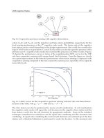
The parasitic coupling level between transmit and receive antennas is a critical parameter in
the design of ground-penetrating radars and satisfactory levels are usually achieved by

empirical design methods. Anyway, the prediction of coupling levels already at the design
stage enhances structure reliability, while also improving design cycle. To this end, the
locally conformal FDTD model presented in Section 2 has been usefully adopted. In this
way, as it can be noticed in Fig. 6, it has been found that the antenna return-loss parameter
11
S is not strongly affected by the buried target which, conversely, has a significant impact
on the frequency behaviour of the coupling level between the radiating elements, due to the
electromagnetic field interference processes occurring at the receiver end.


Fig. 6. Frequency behaviour of the scattering parameters of the dipole antenna pair for
different electrical properties of the buried pipe. Structure characteristics:
40
d
lcm ,
5
d
Dmm , 2.5mm , 20
d
scm , 3
d
hcm , 30
p
Dcm

, 40
p
hcm

.

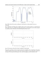
4.1 Analysis of sub-surface scattering processes
The considered antenna pair has been used to analyze the sub-surface scattering
phenomena arising from the field interaction with a PVC pipe buried at a depth
30
p
hcm . As it can be easily inferred, the intensity of the radio signal diffracted by the
pipe and measured at the input terminals of the receive antenna strongly depends on the
electrical and geometrical properties of the target. In particular, the peak-to-peak level of
the signal increases as the diameter, and hence the radar cross section of the pipe becomes
larger (see Fig. 7). Another noticeable phenomenon is the sub-surface excitation of
creeping waves. Such waves, propagating along the pipe surface, give rise to late-time
pulse contributions in the received radio signal which can be clearly noticed in Fig. 7 as
the radius of the object increases. Furthermore, it is worth noting that the strength of the
creeping wave contribution tends to reduce with the pipe size because of the field
attenuation relevant to the extra-path length.
Full-Wave Modelling of Ground-Penetrating Radars:
Antenna Mutual Coupling Phenomena and Sub-Surface Scattering Processes

371


Fig. 7. Time-domain behaviour of the radio signal diffracted by a PVC pipe buried at a
depth
30
p
hcm
in a lossy ground with electrical properties
6
r


 and 15mS m

 . The
effect of the sub-surface excitation of creeping waves can be noticed.
4.2 Impact of ground-embedded inhomogeneities
An invariable feature of real-life soils is heterogeneity. Without taking into account the
inhomogeneities altering the idealized nature of the considered ground model, it becomes a
futile effort to design a complex GPR system that will perform well over a real-life soil. To
overcome this limitation, a realistic ground model has been developed by simulating small
ellipsoidal scatterers embedded in the soil (see Fig. 5). The size, location and electrical
properties of these inhomogeneities are determined randomly within preset limits. In
particular, the maximum dimensions of the scatterers are
10
x
acm

, 10
y
acm , and
2
z
acm in x , y , and z coordinate direction, respectively. In addition, all inhomogeneities
have randomly selected values of the relative permittivity according to the following
Gaussian probability distribution:



2
2
2

2
,
1
,
2
r
r
e










(37)
with mean
13.7

 , and standard deviation 4.2


 (see Fig. 8). As it appears from Fig. 9,
the ground-embedded inhomogeneities have a considerable impact on the coupling
coefficient
21
S of the dipole pair especially at high frequencies ( 0.6

f
GHz ) where the
radiated field assumes a quasi-optical behaviour and the diffraction processes arising from
the interaction with the inhomogeneities tend to be significant, and could mask the
detection of the buried target (see Fig. 10).