Advanced Model Predictive Control Part 5 docx

6
Implementation of Multi-dimensional Model
Predictive Control for Critical Process with
Stochastic Behavior
Jozef Hrbček and Vojtech Šimák
University of Žilina , Faculty of Electrical Engineering, Department of Control and
Information Systems, Žilina
Slovak Republic
1. Introduction
Model predictive control (MPC) is a control method (or group of control methods) which
make explicit use of a model of the process to obtain the control signal by minimizing an
objective function. Control law is easy to implement and requires little computation, its
derivation is more complex than that of the classical PID controllers. The main benefit of
MPC is its constraint handling capacity: unlike most other control strategies, constraints on
inputs and outputs can be incorporated into the MPC optimization (Camacho, E., 2004).
Another benefit of MPC is its ability to anticipate to future events as soon as they enter the
prediction horizon. The implementation supposes good knowledge of system for the
purpose of model creation using the system identification. Modeling and identification as a
methodology dates back to Galileo (1564-1642), who also is important as the founder of
dynamics (Johanson, R., 1993). Identification has many aspects and phases. In our work we
use the parametric identification of real system using the measured data from control centre.
For the purpose of identification it is interesting to describe the sought process using input-
output relations. The general procedure for estimation of the process model consists of
several steps: determination of the model structure, estimation of parameters and
verification of the model. Finally we can convert the created models to any other usable
form. This chapter gives an introduction to model predictive control, and recent
development in design and implementation. The controlled object is an urban tunnel tube.
The task is to design a control system of ventilation based on traffic parameters, i.e. to find
relationship between traffic intensity, speed of traffic, atmospheric and concentration of
pollutants inside the tunnel. Nowadays the control system is designed as tetra - positional
PID controller using programmable logic controllers (PLC). More information about safety

requirements for critical processes control is mentioned in the paper (Ždánsky, J., Rástočný,
K. and Záhradník, J., 2008). The ventilation system should be optimized for chosen criteria.
Using of MPC may lead to optimize the control way for chosen criteria. Even more we can
predict the pollution in the tunnel tube according to appropriate model and measured
values. This information is used in the MPC controller as measured disturbances. By
introducing predictive control it will be made possible to greatly reduce electric power
consumption while keeping the degree of pollution within the allowable limit.

Advanced Model Predictive Control

110
2. Tunnel ventilation system
Emissions from cars are determined not only by the way they are built but also by the way
they are driven in various traffic situations. Various gases are emitted by combustion
engine. They consist largely of oxides of nitrogen (NO
x
), carbon monoxide (CO), steam
(H
2
O) and particles (opacity). Because of these dangerous gases, it is necessary to provide
fresh air in longer tunnels. The fresh air which is used to lower the concentration of CO also
serves to improve visibility. The purpose of ventilation is to reduce the noxious fumes in a
tunnel to a bearable amount by introducing fresh air. Every tunnel has some degree of
natural ventilation. But a mechanical ventilation system should have to be installed. In order
to create air stream, jet fans are installed on the ceiling or side walls of the tunnel. The fans
take in tunnel air and blow it out at higher speed along the axis of the tunnel. In the tunnel
is mounted several fans with about hundred kW each.
The design and industrial implementation of automatic control systems requires powerful
and economic techniques together with efficient tools. In order to solve a control problem it
is necessary to first describe somehow the dynamic behaviors of the system to be controlled.

Traditionally this is done in terms of a mathematical model. Mathematical models are
mathematical expressions of essential characteristics of an existing system that describe
knowledge about the system in a usable form.
Ventilation control system will base on model and sensors information about NO
x
, opacity,
velocity, number of vehicles and CO measurements. According to the amounts of pollutants
in exhaust gas, air flow driven by the vehicles and degree of pollution inside the tunnel,
optimized operation commands will given to the jet fans. “Optimum” means that pollutant
concentration is kept within the allowable limit (for CO, 75 ppm or less), and at the same
time electric power consumption is minimized. Another criterion is also possible, for
example: number of switching the jet fans.
2.1 Tunnel description
The ventilation system in urban tunnel Mrázovka in Prague represents one function unit
designed as longitudinal ventilation with a central efferent shaft and protection system
avoiding spread of harmful pollutants into the tunnel surround area. Ventilation is
longitudinal facing in direction of traffic with air suction at the south opening of the eastern
tube (ETT) and at the branch B, with air being transferred at the north opening to the
western tunnel tube (WTT) (Pavelka, M. and Přibyl, P., 2006). The task is to design a control
system of ventilation based on traffic parameters, i.e. to find relationship between traffic
intensity, speed of traffic, atmospheric and concentration of pollutants inside the tunnel. To
do that the eastern tunnel tube (ETT) has been chosen as a model example due to principle
of mixing polluted air from ETT to WTT (measured concentrations of pollutants in the WTT
are also influenced by traffic intensity in the ETT).
To get the required description, the following data has been taken from the tunnel control
centre: traffic intensity of trucks and cars, their speed, concentrations of CO (carbon
monoxide), NO
x
(oxides of nitrogen), OP (opacity-visibility) from the ETT, atmospheric
pressure etc. These values are measured by sensors installed inside the tunnel (at five

different places of the ETT). Traffic parameters are measured at three places, air flow at
three places and concentrations of NO
x
and atmospheric pressure in the north portal.
Traffic intensity is sensed by a camera system and the cars are then counted and sorted by
categories in database system. More information about monitoring of the traffic can be
found in (Pirník, R., Čapka, M. and Halgaš, J., 2010). About the security by transferring the
data is discussed in (Holečko, P., Krbilová, I., 2006).
Implementation of Multi-dimensional
Model Predictive Control for Critical Process with Stochastic Behavior

111

Traffic
Directio
n
North
Eastern Tunnel Tube (ETT)
South
Branch A
Western Tunnel Tube (WTT)
Branch B
Traffic
Direction
Traffic
Direction
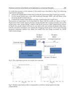
Fig. 1. Simplified diagram of road tunnel (length of 1230m)
3. Mathematical models for MPC
Mathematical models are mathematical expressions of essential characteristics of an existing
or designed system that describe knowledge about the system in a usable form. Turbulence

inside the tunnel, variety of traffic and atmospherics make the system behavior stochastic.
To make the models we use the parametric identification. The MATLABs tools allowed a
conversion between several types of models. The main tasks of system identification were
the choice of model type and model order. For Single-input Multiple-output discrete time
linear systems we can write the metrics equation for jet fan characteristics:

[]
111
2211
231
() ()
() () ()
() ()
yk G k
y
kGkuk
yk G k
 
 
=⋅
 
 
 
(1)
The “Jet Fan Model” is a model in the MPC format that characterizes effect of ventilator on
CO concentration, NO
x
concentration and visibility (opacity). It is a system with 1 input (u)
and 3 outputs (dilution of CO-Out1, NO
x

concentration-Out2 and opacity OP-Out3). One of
the main advantages of predictive control is incorporation of limiting conditions directly to
the control algorithm. The “Jet Fan Model” characteristics are shown in Fig. 2.
The “Disturbance Model” is a model of the tunnel tube in state space representation:

() () () () ()
ttttt uBxAx ⋅+⋅=
′
(2)
() () () () ()
ttttt uDxCy ⋅+⋅=

This model is used to predict the pollutions inside the tunnel tube. These data enter to the
measured disturbances input (MD) of MPC controller for the purpose of switching the jet
fans before the limit will be exceeded.
Created model was validated by several methods (Hrbček, J., 2009). The purpose of model
validation is to verify that identified model fulfills the modeling requirements according to


Advanced Model Predictive Control

112

Fig. 2. Jet fan characteristics

Fig. 2. Model of the tunnel tube. Out 1 – Concentration of CO, Out 2 –OP-opacity inside the
tunnel, Out 3 – Concentration of NOx
subjective and objective criteria of good model approximation. In method “Model and
parameter accuracy” we compare the model performance and behavior with real data. A
deterministic simulation can be used, where real data are compared with the model

response to the recorded input signal used in the identification. This test should ascertain
whether the model response is comparable to real data in magnitude and response delay.


Fig. 3. Model and parameter accuracy test for CO concentrations. Measured data is shown
by black line and simulated data are shown by gray dashed line.

State Space
Model
In 1- cars,
In 2- trucks.
In 3- Velocity
Out 1
Out 2
Out 3
Traffic intensit
y
of:
Implementation of Multi-dimensional
Model Predictive Control for Critical Process with Stochastic Behavior

113
This method showed graphically accuracy between simulated values and measured values.
Although the simulated and measured data not fit precisely, this result is sufficient for most
stochastic system like pollution inside the road tunnel.
An Akaike Final Prediction Error (FPE) for estimated model was also determinate. The
average prediction error is expected to decrease as the number of estimated parameters
increase. One reason for this behavior is that the prediction errors are computed for the data
set that was used for parameter estimation. It is now relevant to ask what prediction
performance can be expected when the estimated parameters are applied to another data

set. This test shows the flexibility of the model structure. We are looking for minimum value
of FPE coefficient.
4. Model predictive control of ventilation system
Under the term “Model Predictive Control” we understand a class of control methods that
have certain characteristic features. MPC refers to a class of computer control algorithms
that utilize an explicit process model to predict the future response of a plant. From this
model the future behaviour of the system is predicted over a finite time interval, usually
called prediction horizon, starting at the current time t.
4.1 The basic idea of predictive control
The receding horizon strategy is shown in Fig. 4.


Fig. 4. The receding horizon strategy, the basic idea of predictive control.
The future outputs for a determined horizon N, called the prediction horizon, are predicted
at each instant t using the process model. These predicted outputs y(t + k|t) 1 for k = 1…N
depend on the known values up to instant t (past inputs and outputs) and on the future
control signals u(t+k|t), k = 0 N-1, which are those to be sent to the system and calculated.
The set of future control signals is calculated by optimizing a determined criterion to keep
the process as close as possible to the reference trajectory w(t + k) (which can be the setpoint
itself or a close approximation of it). This criterion usually takes the form of a quadratic
function of the errors between the predicted output signal and the predicted reference
trajectory. The control effort is included in the objective function in most cases. An explicit
solution can be obtained if the criterion is quadratic, the model is linear, and there are no
constraints; otherwise an iterative optimization method has to be used. Some assumptions
about the structure of the future control law are also made in some cases, such as that it will
be constant from a given instant.
t
t
+1
t

+k …
t
+N
p
as
t

f
uture
y
(
t
)
t
-1
u
(
t
)
w
(
t
)
u
(
t+k|
t
)
y
(

t+k|
t
)
^

Advanced Model Predictive Control

114
The control signal u(t|t) is sent to the process whilst the next control signals calculated are
rejected, because at the next sampling instant y(t+1) is already known and step 1 is repeated
with this new value and all the sequences are brought up to date. Thus the u(t+1|t+1) is
calculated ( which in principle will be different from the u(t+1|t) because of the new
information available) using the receding horizon concept (Camacho, E. F., Bordons, C., 2004).
The notation indicates the value of the variable at the instant t + k calculated at instant t.
4.2 Application to real system
Tunnel ventilation is expected to fulfil the following requirements at least (Godan, J. at
all. 2001):
• Concentration of emissions in the tunnel kept within the acceptable limits for the
monitored harmful pollutants, in consideration of time spent by persons inside the tunnel;
• Good visibility for through passage of vehicles under polluted air inside the tunnel;
• Reduction of effects of smoke and heat on persons in the case of vehicle fire;
• Regulation of dispersion of pollutants in the air caused by petrol fumes from vehicles
into the surround environment of the tunnel.
Model Predictive Control (MPC) comes from the late seventies when it became significantly
developed (Camacho, E. F., Bordons, C., 2004) and several methods were defined. In this
work we have applied the Dynamic Matrix Control (DMC) method which is one of the most
spread approaches and creates the base of many commercially available MPC products. It is
based on the model obtained from the real system:

1

() ( ),
N
i
i
y
khuki
=
=−

(3)
where h
i
are FIR (Finite Impulse Response) coefficients of the model of the controlled
system. Predicted values may be expressed:

ˆ
ˆ
(|) ( )(|)
ˆ
() ()(|)
i
ii
yn k n h un k i dn k n
hunki hunki dnkn
+=Δ+−++=
= Δ +−+ Δ +− + +


(4)
We assume that the additive failure is constant during the prediction horizon:

ˆˆ
ˆ
(|)(|)()(|)
m
dn k n dn n
y
n
y
nn+= = − (5)
Response can be decomposed to the component depending on future values of control and
to the component determined by the system state in time n:

ˆ
(|) ( )(),
i
y
nkn hunki fnk+=Δ+−++

(6)
where f(n+k) is that component which does not depend on future values of action quantity:

()()( )().
nkii
f
nk yn h h uni
+
+= − −Δ −

(7)

Implementation of Multi-dimensional
Model Predictive Control for Critical Process with Stochastic Behavior

115
Predicted values within the prediction horizon p (usually p>>N) can be arranged to the
relation (8):

1
21
ˆ
(1|) ()(1)
ˆ
(2|) () (1)(2)

ˆ
(|) ( )(),
p
i
ipm
yn n h un fn
yn n h un h un f n
y
n
p
nhun
p
i
f
n
p

=− +
+=Δ++
+=Δ+Δ+++
+= Δ+−++

(8)
where the prediction horizon is k=1 p, with respect to m control actions. Regulation circuit
is stable if the prediction horizon is long enough. The values may be arranged to the
dynamic matrix
G:

1
21
11
0 0
0
,
:: :

pp pm
h
hh
G
hh h
−−+
= (9)
and expression used for prediction can be written in the matrix form:

ˆ
,

y
Gu f=+
(10)
where ŷ is a vector of contributions of action quantity and f are free responses.
The MATLAB’s Model Predictive Control Toolbox uses linear dynamic modeling tools. We
can use transfer functions, State-space matrices, or its combination. We can also include
delays, which are in the real system. The model of the plant is a linear time-invariant system
described by the equations:

(1) () ()() ()
() () () ()
() () () (),
uv d
mm vm dm
u u vu du
xk AxkBukBvkBdk
yk Cxk Dvk Ddk
yk Cxk Dvk Ddk
+= + +
=+ +
=+ +
(11)
where x(k) is the n
x
-dimensional state vector of the plant, u(k) is the n
u
-dimensional vector
of manipulated variables (MV), i.e., the command inputs, v(k) is the n
v
-dimensional vector of

measured disturbances (MD), d(k) is the n
d
-dimensional vector of unmeasured disturbances
(UD) entering the plant, y
m
(k) is the vector of measured outputs (MO), and y
u
(k) is the vector
of unmeasured outputs (UO). The overall n
y
-dimensional output vector y(k) collects y
m
(k)
and y
u
(k). In the above equations d(k) collects both state disturbances (B
d
≠0) and output
disturbances (D
d
≠0).
The unmeasured disturbance d(k) is modeled as the output of the linear time invariant
system:

(1) () ()
() () ().
ddd
dd
xk Axk Bnk
dk Cx k Dn k

+= +
=+
(12)
The system described by the above equations is driven by the random Gaussian noise n
d
(k),
having zero mean and unit covariance matrix. For instance, a step-like unmeasured

Advanced Model Predictive Control

116
disturbance is modeled as the output of an integrator. In many practical applications, the
matrices
A, B, C, D of the model representing the process to control are obtained by
linearizing a nonlinear dynamical system, such as

(,,,)
(,,,).
x
f
xuvd
y
hxuvd
′
=
=
(13)
at some nominal value x=x
0
, u=u

0
, v=v
0
, d=d
0
. In these equations x´ denotes either the time
derivative (continuous time model) or the successor x(k+1) (discrete time model).
The MPC control action at time k is obtained by solving the optimization problem:

2
p-1
1,
i0 1
22
2
,,target
11
min ( | ), , ( 1 | ), ( ( 1| ) ( 1))
(|) ((|) ())
(
)
{[
]},
z
uu
n
u
ijj j
j
nn

u
ij j ij j j
ii
uk k um k k w y k i k r k i
wukik wukiku ki
ε
ε
ρε
+
==
Δ
==
ΔΔ−+ ++−++
+Δ++ +− ++


(14)
where the subscript "( )j" denotes the j-th component of a vector, "(k+i|k)" denotes the value
predicted for time k+i based on the information available at time k; r(k) is the current sample
of the output reference, subject to

min min max max
min min max max
min max
min max
() () ( | ) () ();
() () ( | ) () ();
() () ( 1| ) () (),
(|)0,
0, , 1,

, , 1,
uu
jjj j j
uu
jj j jj
yy
jjj
jj
uiViukikuiVi
uiViukikuiVi
y
iV i
y
ki k
y
iV i
uk h k
where
ip
hm p
εε
εε
εε
ε
ΔΔ
−≤+≤+
Δ− ≤Δ+≤Δ+
−≤++≤+
Δ+ =
=−

=−
≥ 0,
(15)
with respect to the sequence of input increments {
( | ), , ( 1 | )ukk um kkΔΔ−+
} and to the slack
variable ε, and by setting u(k)=u(k-1)+ Δu(k|k), where Δu(k|k) is the first element of the
optimal sequence. Note that although only the measured output vector y
m
(k) is fed back to
the MPC controller, r(k) is a reference for all the outputs. When the reference r is not known
in advance, the current reference r(k) is used over the whole prediction horizon, namely
r(k+i+1)=r(k) in Equation 14.
In Model Predictive Control the exploitation of future references is referred to as anticipative
action (or look-ahead or preview). A similar anticipative action can be performed with respect
to measured disturbances v(k), namely v(k+i)=v(k) if the measured disturbance is not known in
advance (e.g. is coming from a Simulink block) or v(k+i) is obtained from the workspace. In the
prediction, d(k+i) is instead obtained by setting n
d
(k+i)=0. The w
Δu
ij, w
u
ij, w
y
ij, are nonnegative
weights for the corresponding variable. The smaller w, the less important is the behavior of the
corresponding variable to the overall performance index. And u
j,min
, u

j,max
, Δu
j,min
, Δu
j,max
, y
j,min
,
y
j,max
are lower/upper bounds on the corresponding variables. The constraints on u, Δu, and y
are relaxed by introducing the slack variable ε≥ 0. The weight ρε on the slack variable ε
Implementation of Multi-dimensional
Model Predictive Control for Critical Process with Stochastic Behavior

117
penalizes the violation of the constraints. The larger ρε with respect to input and output
weights, the more the constraint violation is penalized. The Equal Concern for the Relaxation
vectors V
u
min
,V
u
max
, V
Δu
min
, V
Du
max

, V
y
min
, V
y
max
have nonnegative entries which represent the
concern for relaxing the corresponding constraint; the larger V, the softer the constraint. V=0
means that the constraint is a hard one that cannot be violated (Bemporad A., Morari M., N.
Lawrence Ricker., 2010).
4.3 Constraints
In many control applications the desired performance cannot be expressed solely as a
trajectory following problem. Many practical requirements are more naturally expressed as
constraints on process variables. There are three types of process constraints: Manipulated
Variable Constraints: these are hard limits on inputs u(k) to take care of, for example, valve
saturation constraints; Manipulated Variable Rate Constraints: these are hard limits on the
size of the manipulated variable moves Δu(k) to directly influence the rate of change of the
manipulated variables; Output Variable Constraints: hard or soft limits on the outputs of the
system are imposed to, for example, avoid overshoots and undershoots (Maciejovski,
J.M., 2002). We use the Output constraints and Manipulated Variable Constraints.

5. Simulation in MATLAB
Models of the tunnel and ventilator have been obtained through identification of real
equipments. Higher traffic intensity causes increase of pollutant concentrations in the
tunnel. This intensity is expressed as a vector containing really measured data. The
MATLAB environment is used to simulate behavior of the system according to the Fig. 5.


Traffic Intensity,
Velocity and Atmospherics

Tunnel Tube
Disturbances Model

MPC
Controller
Required
value
u
Jet Fan
+
+
y – Output
(CO, NO
x
and Visibility)
w
r

Measured Disturbance
with predictions
w‘
Constraints

Fig. 5. Improved MPC of multi-dimensional ventilation system
It is a closed-loop control (regulation) of the system with limitations imposed to control
quantity and outputs. It uses the internal model and solves optimization problem with the
use of quadratic programming. We can choose the prediction horizon P and the control
horizon M. The output constraints were set to 6, because this is the maximum input for three
pairs of jet fans corresponding with real system. Weight matrix is selected as a diagonal
matrix, with each element weighting the corresponding control signal. For instance, if the

influence of particular control is to be reduced, then the corresponding diagonal element
will be increased to reflect this intention. Weight tuning is the essential task to set the
controller. In Fig. 7 we can see the results in comparison to Fig. 6.

Advanced Model Predictive Control

118

Fig. 6. Simulated values of CO pollution inside the tunnel with (grey line) and without
(black line) MPC controller and fan number (number of acting jet fans)
5.1 Simulation results
The presented simulation results are obtained for the following concentration limits: 6
ppm for CO concentrations, 0.02 ppm for NOx concentrations and 0.05 ppm for
visibility concentrations. These values are below really defined maximum limits.
According to the curve of the output quantity (Fig. 6) it is apparent, that no emission
value has extended the defined limit. However, the value of under-set maximum limit
may be extended since one ventilator need not be able to dilute CO concentration
sufficiently.
The abbreviation ppm is a way of expressing very dilute concentrations of substances. Just
as per cent means out of a hundred, so parts per million or ppm means out of a million. It
describes the concentration of something in air.
For this simulation we have six acting jet fans in this part of road tunnel. In the next
simulations we have used a possibility to set weighing matrices (uwt) for tuning the
controller. The control quantity u is adapted to the input of Jet Fan control unit. The black
lines represent the concentrations of pollution without using the controller. They are
named CO. The grey lines represent the concentrations of pollution with using the
controller. They are named COr. Opacity and concentration of NO
x
is below the
dangerous limits. The jet fans were switched on two times per day for chosen limits. We

can see how affect the ventilation system to reduce the pollution. In this paper we pointed
out only to concentration of CO, because this type of pollution is most dangerous for
human organism.
As it was mentioned in the previous section the weight tuning is also important part of
controller creation.
Well tuned controller leads to optimal control. After changing the weights, the jet fans were
switched on only once per day, furthermore the next day all the fans were not switched on
in the same conditions.
Implementation of Multi-dimensional
Model Predictive Control for Critical Process with Stochastic Behavior

119

Fig. 7. Weight tuning. Simulated values of CO pollution inside the tunnel with (grey line)
and without (black line) MPC controller and fan number (number of acting jet fans)
Opacity and concentration of NO
x
is below the dangerous limits. The jet fans were switched
on once per day for chosen limits. The concentrations of NO
x
and opacity (OP) are shown in
Fig. 8.


Fig. 8. Simulated values of NO
x
concentrations inside the tunnel tube (black line) and
opacity (grey line)
For this simulation the NO
x

concentrations and opacity was below defined maximum limits.
When the jet fans are switched on these pollutions are also decreased.
5.2 Implementation
The biggest advantage of Automatic Code Generation affects those developers who already
use MATLAB and Simulink for simulation and solutions design and to developers who
used to tediously rework implemented structures in a language supported by Automation
Studio in the past. In the procedures listed below the Automatic Code Generation tool
provided by B&R represents an innovation with endless possibilities that help to
productively reform the development of control systems. The basic principle is simple: The
module created in Simulink is automatically translated using Real-Time Workshop and
Real-Time Workshop Embedded Coder into the optimal language for the B&R target system

Advanced Model Predictive Control

120
guaranteeing maximum performance of the generated source code. Seamless integration
into an Automation Studio project makes the development process perfect (B&R
Automation Studio Target for Simulink. 2011). Since the tunnel ventilation system use
programmable logic controllers (PLC) it is suitable for real implementation. In our
department we have appropriate equipment for this solution.


Fig. 9. Workflow of the Automatic Code Generation
The elimination of extensive reengineering in Automation Studio allows simple transfer of
complex and sophisticated Simulink models to the PLC (Hardware-in-the-Loop). Closed-
loop controllers can also be easily tested and optimized on the target system without
requiring the user to adjust large amounts of code and run the risk of creating coding errors
(Rapid Prototyping). Rapid prototyping: Automatic Code Generation makes it possible to
quickly and easily transform sophisticated Simulink based control systems into source code
and integrate them into an Automation Studio project. Many potentially successful ideas

have been immediately rejected due to the large amount of time required for conversion into
executable machine code and the risk of developing a dead end solution.
The “Rapid Prototyping” concept brings an end to this. Using Simulink and the Automatic
Code Generation tool provided by B&R, any system, no matter how complex, can be
intuitively built, compiled and tested in a short amount of time. This practically eliminates
implementation errors as the Automatic Code Generation tool has been well-proven over
several years in critical fields like aviation or automotive industry (B&R Automation Studio
Target for Simulink. 2011). Nowadays the control algorithm is implemented and awaiting
for connection to the real system. Fig. 11. shows the model in Simulink.
We created the model in Simulink according to model for simulations. We replaced the
simulated inputs by “B&R IN” blocks and simulated output by the “B&R OUT” block. The
Real-time Workshop provides utilities to convert the SIMULINK embedded models in C
code and then, with the compiler, compile the code into a real-time executable file. Although
the underlying code is compiled into a real-time executable file via the C compiler, this
conversion is performed automatically without much input from the user. The concept in
Simulink Model
Automation Studio
Project
Automation
System (PLC)
C code
C code
Implementation of Multi-dimensional
Model Predictive Control for Critical Process with Stochastic Behavior

121
Fig. 10. shows that a simulation model can be used in the simulation testing of the predictive
control system, and after completing the test, then with simple modification to the original
Simulink programs, the same real-time predictive control system can be connected to the
actual plant for controlling the plant.

Fig. 10. The control system




Fig. 11. The control system in Simulink

Advanced Model Predictive Control

122
6. Conclusion
The paper presents a methodology that has been used for design parametric models of the
road tunnel system. We needs identification of system based on data obtained from the real
ventilation system. Model from one week data has been created and verified in MATLAB
environment. This part is the ground for best design of ventilation control system. Presented
results point out that created model by identification method should be validate by several
method. Model of a three-dimensional system has been created and simulated in MATLAB
environment using the predictive controller. Presented results confirm higher effectiveness
of predictive control approach. The weight tuning is important part of controller creation as
the simulation results had proved. The predictive controller was successfully implemented
to programmable logic controller.
7. Acknowledgment
This paper was supported by the operation program “Research and development” of
ASFEU-Agency within the frame of the project "Nové metódy merania fyzikálnych
dynamických parametrov a interakcií motorových vozidiel, dopravného prúdu a vozovky".

ITMS 26220220089 OPVaV-2009/2.2/03-SORO co financed by European fond of regional
development. “We support research activities in Slovakia / The project is co financed by
EU”.

8. References
Camacho, E. F., Bordons, C. (2004). Model Predictive Control. 2nd ed., Springer-Verlag
LondonLimited, 405 p. ISBN 1-85233-694-3
Maciejovski, J.M. (2002). Predictive Control with constrains, Prentice Hall, 331p, ISBN: 0-201-
39823-0
Ždánsky, J., Hrbček, J., Zelenka, J. (2008) Trends in Control Area of PLC Reliability and
Safety Parameters, ADVANCES in Electrical and Electronic Engineering, ISSN 1336-
1376, Vol.7/2008, p. 239-242
Johanson, R. (1993). System modeling and identification, Prentice-Hall, 512p., ISBN: 0-13-
482308-7
Hrbček, J. and Janota, A. (2008). Improvement of Road Tunnel Ventilation through
Predictive Control, Communications, 2/2008, p.15-19, ISSN: 1335-4205
Pavelka, M Přibyl, P. (2006). Simulation of Air Motion and pollutions inside the Road Tunnel–
Mathematical Model. OPTUN 228/06-EEG
EN 61508. (2002). Functional safety of electrical/electronic/programmable electronic safety-
related systems.
Bemporad A., Morari M. N. Lawrence Ricker. (2010). Model Predictive Control Toolbox.
Available from:
Implementation of Multi-dimensional
Model Predictive Control for Critical Process with Stochastic Behavior

123
Vojtech Veselý and Danica Rosinová. (2010). Robust Model Predictive Control Design, In:
Model Predictive Control, 87-108, Scyio, ISBN 978-953-307-102-2, Available from

Godan, J. at all. (2001). Tunnels, Road Tunnels and Railway Tunnels, p. 202. 135882/p-UK/Z

Liuping Wang. (2009) Model Predictive Control System Design and Implementation Using
MATLAB, Springer, p. 371, ISBN 978-1-84882-330-3
Hrbček, J. (2009). Parametric Models of Real System and the Validation Tools. Proceeding of
8th European Conference of Young Research and Science Workers in Transport and
Communications technology. p. 93-96. Žilina: June, 22. – 24. 2009. ISBN 978-80-554-
0027-3
Pirník, R., Čapka, M. and Halgaš, J. (2010). Non-invasive monitoring of calm traffic.
Proceedings of international symposium on advanced engineering & applied management –
40th anniversary in higher education, CD ver. S. II-107-112, ISBN 978-973-0-09340-7
B&R Automation Studio Target for Simulink. (2011). Available from:
/>53.html
Bubnicki, Z. (2005). Modern Control Theory. Springer, 2005, 422 p., ISBN 3-540-23951-0
Tammi, K. (2007). Active control of radial rotor vibrations, Picaset Oy, Helsinki 2007, VTT, ISBN
987-951-38-7007-2
Hrbček, J., Spalek J. and Šimák, V. (2010). Process Model and Implementation the
Multivariable Model Predictive Control to Ventilation System. Proceeding of 8th
International Symposium on Applied Machine Intelligence and Informatics, CD, p. 211-
214, Herľany, Slovakia, January 28-30, 2010, ISBN 978-1-4244-6423-4
Rossiter J. A. (2003). Model-Based Predictive Control: A Practical Approach. Crc press, 318 p.,
ISBN 0-8493-1291-4
Holečko, P., Krbilová, I. (2006). IT Security Aspects of Industrial Control Systems. Advances
in Electrical and Electronic Engineering, No. 1-2 Vol. 5/2006, pp. 136-139, ISSN 1336-
1376
Ždánsky, J., Rástočný, K. and Záhradník,J. (2008). Problems Related to the PLC Application
in the Safety Systems. Trudy rostovskogo gosudarstvennogo universiteta putej
soobščenija, No. 2(6) 2008, pp. 109–116, ISSN 1818–5509
Lewis, P. – Yang, Ch. (1997). Basic Control Systems Engineering, 1997, Prentice-Hall, ISBN 0-
13-597436-4
Přibyl, P., Janota, A. and Spalek, J. (2008). Analýza a řízení rizik v dopravě. Pozemní komunikace
a železnice. (Analysis and risk control in transport. Highway and railway). BEN Praha,

ISBN 80-7300-214-0
Noskievič, P. (1999). Modelování a identifikace systémů. (Systems modeling and identification).,
Ostrava: MONTANEX, a.s., 1999, 276 p., ISBN 80-7225-030-2
Balátě, J. (2004). Automatické řízení. (Automation control). BEN, Praha, 2004, ISBN 80-7300-148-9
Zelenka, J. – Matejka, T. (2010). The application of discrete event systems theory for the real
manufacturing system analysis and modeling. Proceedings of the conference of
cybernetics and informatics 2010, Vyšná Boca 2010, ISBN 978-80- 227-3241-3
Yinghua He, Hong Wang, and Bo Zhang. (2004). Color-Based Road Detection in Urban
Traffic Scenes, IEEE Transactions on intelligent transportation systems, vol. 5, no. 4,
december 2004. Available from:


Advanced Model Predictive Control

124
Harsányi L., Murgaš J., Rosinová D., Kozáková A. (1998). Teória automatického
riadenia.(Automation system theory). STU Bratislava, Bratislava 1998, ISBN 80-227-
1098-9
Hrbček, J. (2007). Active Control of Rotor Vibration by Model Predictive Control – a simulation
study. Report 153, Picaset Oy, Helsinki 2007, ISSN: 0356-0872, ISBN: 978-951-22-
8824-3
Ma Y., Soatto S., Košecká J., Sastry S. S. (2004). An Invitation to 3-D Vision – From Images to
Geometric Models. Springer - Verlag New York, Inc., New York 2004, ISBN 978-0387-
00893-6
Šimák, V., Hrbček, J., Pirník, R. (2010). Traffic flow videodetection, International conference
KYBERNETIKA A INFORMATIKA ´10, Vyšná Boca, Slovakia, February 10-13, 2010,
ISBN 978-80-227-3241-3
7
Fuzzy–neural Model Predictive Control of
Multivariable Processes

Michail Petrov, Sevil Ahmed, Alexander Ichtev and Albena Taneva
Technical University Sofia, Branch Plovdiv/Control Systems Department
Bulgaria
1. Introduction
Predictive control is a model-based strategy used to calculate the optimal control action, by
solving an optimization problem at each sampling interval, in order to maintain the output
of the controlled plant close to the desired reference. Model predictive control (MPC) based
on linear models is an advanced control technique with many applications in the process
industry (Rossiter, 2003). The next natural step is to extend the MPC concept to work with
nonlinear models. The use of controllers that take into account the nonlinearities of the plant
implies an improvement in the performance of the plant by reducing the impact of the
disturbances and improving the tracking capabilities of the control system.
In this chapter, Nonlinear Model Predictive Control (NMPC) is studied as a more applicable
approach for optimal control of multivariable processes. In general, a wide range of
industrial processes are inherently nonlinear. For such nonlinear systems it is necessary to
apply NMPC. Recently, several researchers have developed NMPC algorithms (Martinsen et
al., 2004) that work with different types of nonlinear models. Some of these models use
empirical data, such as artificial neural networks and fuzzy logic models. The model
accuracy is very important in order to provide an efficient and adequate control action.
Accurate nonlinear models based on soft computing (fuzzy and neural) techniques, are
increasingly being used in model-based control (Mollov et al., 2004).
On the other hand, the mathematical model type, which the modelling algorithm relies on,
should be selected. State-space models are usually preferred to transfer functions, because
the number of coefficients is substantially reduced, which simplifies the computation;
systems instability can be handled; there is no truncation error. Multi-input multi-output
(MIMO) systems are modelled easily (Camacho et al., 2004) and numerical conditioning is
less important.
A state-space representation of a Takagi-Sugeno type fuzzy-neural model (Ahmed et al.,
2010; Petrov et al., 2008) is proposed in the Section 2. This type of models ensures easier
description and direct computation of the gradient control vector during the optimization

procedure. Identification procedure of the proposed model relies on a training algorithm,
which is well-known in the field of artificial neural networks.
Obtaining an accurate model is the first stage of the of the NMPC predictive control
strategy. The second stage involves the computation of a future control actions sequence. In
order to obtain the control actions, a previously defined optimization problem has to be
solved. Different types of objective and optimization algorithms (Fletcher, 2000) can be used

Advanced Model Predictive Control

126
in the optimization procedure. Two different approaches for NMPC are proposed in Section
3. They consider the unconstrained and constrained model predictive control problem. Both
of the approaches use the proposed Takagi-Sugeno fuzzy-neural predictive model.
The proposed techniques of fuzzy-neural MPC are studied in Section 4, by experimental
simulations in Matlab
®
environment in order to control the levels in a multi tank system
(Inteco, 2009). The case study is capable to show how the proposed NMPC algorithms
handle multivariable processes control problem.
2. Multivariable fuzzy-neural predictive model
The Takagi-Sugeno fuzzy-neural models are powerful modelling tools for a wide class of
nonlinear systems. Fuzzy reasoning is capable of handling uncertain and imprecise
information while neural networks can learn from samples. Fuzzy-neural networks combine
the advantages of both artificial intelligent techniques and incorporate them in adaptive
features. Those futures, based on a real time learning algorithm are the main advantage of
the fuzzy-neural models.
The importance of the used in MPC strategy models and their adaptive characteristics is
obvious. The accuracy of the model determines the accuracy of the control action. The
proposed fuzzy-neural model is implemented in a classical NMPC scheme (Fig. 1) as a
predictor (Camacho et al., 2004).

Fig. 1. Basic structure of the proposed Fuzzy-Neural NMPC
In this chapter a nonlinear discrete time state-space implementation is considered to
represent the system dynamic:

1,
,
x
y
x(k ) f (x(k) u(k))
y(k) f (x(k) u(k))
+=
=
(1)
where x(k)
∈
n
ℜ
, u(k) ∈
m
ℜ
and y(k) ∈
q
ℜ
are state, control and output variables of the
system, respectively. The unknown nonlinear functions f
x
and f
y

can be approximated by
Takagi-Sugeno type fuzzy rules in the next form:

Fuzzy–neural Model Predictive Control of Multivariable Processes

127

11
:() () ()
(1) () ()
() () ()
l
lili
p
l
p
lll
ll l
R if z k is M and and z k is M and z k is M
xk Axk Buk
then
yk Cxk Duk
+= +



=+




(2)
where R
l
is the l
-th
rule of the rule base. Each rule is represented by an if-then conception.
The antecedent part of the rules has the following form “z
i
(k) is M
li
” where z
i
(k)

is an i
-th

linguistic variable (i
-th
model input) and M
li
is a membership function defined by a fuzzy set
of the universe of discourse of the input z
i
. Note that the input regression vector z(k) ∈
p
ℜ in
this chapter contains the system states and inputs
z(k)=[x(k) u(k)]
T

. The consequent part of
the rules is a mathematical function of the model inputs and states. A state-space
implementation is used in the consequent part of R
l
, where A
l
∈
nn×
ℜ , B
l ∈
nm×
ℜ
, C
l ∈
q
n×
ℜ
and D
l ∈
q
m×
ℜ
are the state-space matrices of the model (Ahmed et al., 2009).
The states in the next sampling time
ˆ
(1)xk+
and the system output
ˆ
()
y

k can be obtained by
taking the weighted sum of the activated fuzzy rules, using

1
1
ˆ
( 1) ()( () ())
ˆˆ
() ()( () ())
L
yl l l
l
L
yl l l
l
xk k Axk Buk
yk k Cxk Duk
μ
μ
=
=
+= +
=+


(3)
On the other hand the state-space matrices A, B, C, and D for the global state-space plant
model could be calculated as a weighted sum of the local matrices A
l
, B

l
, C
l
,

and D
l
from the
activated fuzzy rules (2):

11
11
() () B() ()
( ) ( ) D( ) ( )
LL
lyl lyl
ll
LL
lyl lyl
ll
Ak A k k B k
Ck C k k D k
μμ
μμ
==
==
==
==



(4)
where
1
L
y
l
y
l
y
l
l
μμ μ
=
=

is the normalized value of the membership function degree μ
yl
upon
the l
-th
activated fuzzy rule and L is the number of the activated rules at the moment k.


Fig. 2. Gaussian membership functions of the i
-th
input
Fuzzy implication in the l
-th
rule (2) can be realized by means of a product composition

Advanced Model Predictive Control

128

1
p
y
li
j
i
μμ
=
=
∏
(5)
where μ
ij
specifies the membership degree (Fig. 2) upon the activated j
-th
fuzzy set of the
corresponded i
-th
input signal and it is calculated according to the chosen here Gaussian
membership function (6) for the l
-th
activated rule:

2
2
()

()exp
2
iGi
j
ij i
ij
zc
z
μ
σ
−
=−
(6)
where z
i
is the current input value of the i
-th
model input, c
Gij
is the centre (position) and σ
ij
is
the standard deviation (wide) of the j
-th
membership function (j=1, 2, , s) (Fig.2).
2.1 Identification procedure for the fuzzy–neural model
The proposed identification procedure determines the unknown parameters in the Takagi-
Sugeno fuzzy model, i.e. the parameters of membership functions, according to their shape
and the parameters of the functions f
x

and f
y
in the consequent part of the rules (2). It is
realised by a five-layer fuzzy-neural network (Fig. 3). Each of the layers performs typical
fuzzy logic strategy operations:


Fig. 3. The structure of the proposed fuzzy - neural model
Layer 1. The first layer represents the model inputs through its own input nodes Z
1
, Z
2
, …,
Z
p
. The network synaptic weights are set to one, so the model inputs are directly passed
through the nodes to the next layer. Neurons here are represented by the elements of the
regression vector
z(k).

Fuzzy–neural Model Predictive Control of Multivariable Processes

129
Layer 2. The fuzzification procedure of the input variables is performed in the second layer.
The weights in this layer are the parameters of the chosen membership functions. Their
number depends on the type and the number of the applied functions. All these parameters

ij
are adjustable and take part in the premise term of the Takagi-Sugeno type fuzzy rule
base (2). In that section the membership functions for each model input variable are

represented by Gaussian functions (Fig. 2). Hence, the adjustable parameters 
ij
are the
centres c
Gij
and standard deviations σ
ij
of the Gaussian functions (6). The nodes in the second
layer of the fuzzy-neural architecture represent the membership degrees μ
ij
(z
i
) of the
activated membership functions for each model input z
i
(k) according to (6). The number of
the neurons depends on the number of the model inputs p and the number of the
membership functions s in corresponding fuzzy sets. It is calculated as
p
s× .
Layer 3. The third layer of the network interprets the fuzzy rule base (2). Each neuron in the
third layer has as many inputs as the input regression vector size p. They are the corresponding
membership degrees for the activated membership functions calculated in the previous layer.
Therefore, each node in the third layer represents a fuzzy rule R
l
, defined by Takagi-Sugeno
fuzzy model. The outputs of the neurons are the results of the applied fuzzy rule base.
Layer 4. The fourth layer implements the fuzzy implication (5). Weights in this layer are set
to one, in case the rule R
l

from the third layer is activated, otherwise weights are zeros.
Layer 5. The last layer (one node layer) represents the defuzzyfication procedure and forms
the output of the fuzzy-neural network (3). This layer also contains a set of adjustable
parameters – β
l
. These are the parameters in the consequent part of Takagi-Sugeno fuzzy
model (2). The single node in this layer computes the overall model output signal as the
summation of all signals coming from the previous layer.

5
1
L
y
l
y
l
l
If
μ
=
=

or
5
1
L
xl
y
l
l

If
μ
=
=


5
1
1
L
y
l
y
l
l
L
y
l
l
f
O
μ
μ
=
=
=


or
5

1
1
L
xl
y
l
l
L
y
l
l
f
O
μ
μ
=
=
=


(7)
where
() ()
xl l l
fAxkBuk=+ and () ()
yl l l
f
Cxk Duk=+.
2.2 Learning algorithm of the fuzzy–neural model
Two-step gradient learning procedure is used as a learning algorithm of the internal fuzzy-

neural model. It is based on minimization of an instant error function E
FNN
. At time k the
function is obtained from the following equation

2
() ()/2
FNN
Ek k
ε
=
(8)
where the error ε(k) is calculated as a difference between the controlled process output y(k)
and the fuzzy-neural model output ŷ(k):

ˆ
() () ()kykyk
ε
=− (9)
During step one of the procedure, the consequent parameters of Takagi-Sugeno fuzzy rules
are calculated according to summary expression (10) (Petrov et al., 2002).

(1) ()
FNN
ll
l
E
kk
ββη
∂β


∂
+= + −


(10)

Advanced Model Predictive Control

130
where η is a learning rate and β
l
represents an adjustable coefficient a
ij
, b
ij
, c
ij
, d
ij
(11) for the
activated fuzzy rule R
l
(2). The coefficients take part in the state matrix A
l
, control matrix B
l

and output matrices C
l

and D
l
of the l
-th
activated rule (Ahmed et al., 2009). The matrices

approximate the unknown nonlinear functions f
x
and f
y
according to defined fuzzy rule
model (2). The matrix dimensions are specified by the system parameters – numbers of
inputs m, outputs q and states n of the system.

11 1 11 1 11 1 11 1
11 1 1
nmn m
ll ll
nnn nnm
qq
n
qq
m
aa bb cc dd
ABCD
aa bb cc dd

 



 

== ==

 


 



 
 
      
 
(11)
In order to find a weight correction for the parameters in the last layer of the proposed
fuzzy-neural network the derivative
FNN
l
E
∂
β
∂
of the instant error should be determined.
Following the chain rule, the derivative is calculated considering the expressions (7) and (8)

5
5
ˆ

ˆ
FNN FNN
ll
y
EE
I
y
I
∂
∂∂
∂
∂
β
∂∂
β
∂
=⋅⋅
(12)
After the calculation of the partial derivatives, the matrix elements for each matrix of the
state-space equations corresponding to the
l
-th
activated rule (2) are obtained according to
the summary expression (12) (Petrov et al., 2002; Ahmed et al., 2010):

( 1) ( ) ( ) ( ) ( ) 1
( 1) ( ) ( ) ( ) ( ) 1 , 1
( 1) ( ) ( ) ( ) ( ) 1 , 1
( 1) ( ) ( ) ( ) ( ) 1 ,
ij ij yl i

ij ij yl j
ij ij yl j
ij ij yl j
ak ak k kxk i j n
bk bk k kuk i nj m
ck ck kkxk iqjn
dk dk k kuk i qj
ηε μ
ηε μ
ηε μ
ηε μ
+= + ==÷
+= + =÷ =÷
+= + =÷ =÷
+= + =÷ =1 m÷
(13)
The proposed fuzzy-neural architecture allows the use of the previously calculated output
error (8) in the next step of the parameters update procedure. The output error
E
FNN
is
propagated back directly to the second layer, where the second group of adjustable
parameters are situated (Fig. 3). Depending on network architecture, the membership
degrees calculated in the fourth and the second network layer are related as
μ
yl
→ μ
ij
.
Therefore, the learning rule for the second group adjustable parameters can be done in

similar expression as (10):

(1) ()
FNN
ij ij
ij
E
kk
ααη
∂α

∂

+= +−


(14)
where the derivative of the output error
E
FNN
is calculated by the separate partial
derivatives:

ˆ
ˆ
i
j
FNN FNN
i
j

i
j
i
j
y
EE
y
∂
μ
∂
∂∂
∂α ∂ ∂
μ
∂α
=⋅⋅
(15)

Fuzzy–neural Model Predictive Control of Multivariable Processes

131
The adjustable premise parameters of the fuzzy-neural model are the centre c
Gij
and the
deviation
σ
ij
of the Gaussian membership function (6). They are combined in the
representative parameter 
ij
, which corresponds to the i

-th
model input and its j
-th
activated
fuzzy set. Following the expressions (14) and (15) the parameters are calculated as follows
(Petrov et al., 2002; Ahmed et al., 2010):

2
[() ()]
(1) () ()()[ ()]
()
iGij
Gij Gij yl yl
ij
zk c k
ck ck k kf yk
k
ηε μ
σ
−
+= + −

(16)

2
3
[() ()]
(1) () ()()[ ()]
()
iGij

ij ij yl yl
ij
zk c k
kkkkfyk
k
σσηεμ
σ
−
+= + −

(17)
The proposed identification procedure for the fuzzy-neural model could be summarized in
the following steps (Table 1).

Step 1. Initialize the membership functions – number, shape, parameters;
Step 2. Assign initial values for the network inputs;
Step 3. Start the algorithm at the current moment k;
Step 4. Fuzzify the network inputs and calculate the membership degrees upon the
activated fuzzy set of the membership functions according to (6);
Step 5. Perform fuzzy implication according to (5);
Step 6. Calculate the fuzzy-neural network output, which is represented by state-space
description of the modelled system – (3) and (4);
Step 7. Calculate the instant error according to (8) and (9);
Step 8. Start training procedure for fuzzy-neural network;
Step 9. Adjust the consequent parameters according to (13);
Step 10. Adjust the premise parameters according to (16) and (17).
Repeat the algorithm from Step 3 for each sampling time.
Table 1. Fuzzy-neural model identification procedure
3. Optimization algorithm of multivariable model predictive control strategy
The model provided by the Takagi-Sugeno type fuzzy-neural network is used to formulate

the objective function for the optimization algorithm and to calculate the future control
actions. The second stage of the predictive control strategy includes an optimization
procedure. It utilizes the obtained results during the first (modelling) stage predictive model
of the system. Using the Takagi-Sugeno fuzzy-neural model (3), the optimization algorithm
computes the future control actions at each sampling period, by minimizing the typical for
MPC strategy (Generalized Predictive Control – GPC) cost function (Akesson, 2006):

1
1
2
2
0
ˆ
() ()() ()
pw
u
w
HH
H
R
Q
iH i
Jk yk i rk i uk i
+−
−
==
=+−++Δ+




(18)
where ŷ(k), r(k) and ∆u(k) are the predicted outputs, the reference trajectories, and the
predicted control increments at time k, respectively. The length of the prediction horizon is

Advanced Model Predictive Control

132
H
p
, and the first sample to be included in the horizon is H
w
. The control horizon is given by
H
u
. Q

≥0 and R

>0 are weighting matrices representing the relative importance of each
controlled and manipulated variable and they are assumed to be constant over the
H
p
.
The cost function (18) may be rewritten in a matrix form as follows

22
() () () ()
QR
Jk Yk Tk Uk=− +Δ
(19)

where
Y(k), T(k), ∆U(k), Q and R are predicted output, system reference, control variable
increment and weighting matrices, respectively,
ˆ
(|) (|) (|)
( ) , ( ) , ( )
ˆ
( - 1| ) ( - 1| ) ( - 1| )
pp u
yk k rk k uk k
Yk Tk Uk
y
kH k rkH k ukH k

Δ





==Δ=






++Δ+




 

(1) 0
0()
p
Q
Q
QH






=








 



(1) 0
0()

u
R
R
RH




=








 



The linear state-space model used for Takagi-Sugeno fuzzy rules (2) could be represented in
the following form:

ˆ
(1) () (1) ()
ˆˆ
() () ( 1) ()
xk Axk Buk B uk
y

kCxkDuk Duk
+= + −+Δ
=+−+Δ
(20)
Based on the state-space matrices A, B, C and D (4), the future state variables are calculated
sequentially using the set of future control parameters:
2
32 2
ˆ
(1) () (1) ()
ˆ
(2) ()( )(1)( )() (1)
ˆ
(3) ()( )(1)( )()( )(1) (2)

xk Axk Buk B uk
xk Axk AB Buk AB B uk B uk
xk Axk ABABBuk ABABBuk ABBuk Buk
+= + −+Δ
+= + + −+ +Δ +Δ +
+= + + + −+ + +Δ + +Δ ++Δ +
111
000

ˆ
() () (1) ( )

jjji
j
ii

iim
xk j Axk ABuk AB uk m
−−−−
===
+= + −+ Δ +

112
000

ˆ
() () (1) () (1) ( 1)
ppp
p pu
HHH
H HH
iii
p u
iii
xk H A xk ABuk ABuk ABuk A B uk H
−−−
−
===
+= + −+ Δ+ Δ+++ Δ+−




The predictions of the output
ˆ
y

for j steps ahead could be calculated as follows
2
ˆ
( 1) ( 1) ( 1) ( ) ( ) ( 1) ( ) ( ) ( 1)
ˆ
(2) ()( )(1)( )()( )(1) (2)

y k Cx k Du k CAx k CB D u k CB D u k D u k
y k CA x k CAB CB D u k CAB CB D u k CB D u k D u k
+= ++ += + + −+ +Δ +Δ +
+= +++ −+++Δ++Δ++Δ+



Fuzzy–neural Model Predictive Control of Multivariable Processes

133
11
00
ˆ
() () (1) ()( )( 1) ()

jj
j
ii
ii
y k j CAx k C AB D uk C AB D uk CB D uk j D uk j
−−
==


+= + + −+ + Δ + + Δ +−+Δ +




22
1
00
31
00

ˆ
(1) () (1) ()
(1)
pp
p
ppu
HH
H
ii
p
ii
HHH
ii
ii
yk H CA xk C AB Duk C AB D uk
CABDuk C ABD
−−
−
==

−−−
==


+−= + + −+ +Δ +


  
  
++Δ+++ +
  
  


 (1)
u
uk HΔ+ −

The recurrent equation for the output predictions
ˆ
()
p
y
k
j
+
, where j
p
= 1, 2, , H
p

–1
,
is in the
next form:
.
1
1
00
1
1
0
00
(),
ˆ
() () (1)
(),
pp
p
p
p
u
jj
j
pu
j
ij
j
i
p
ji

H
i
j
p
u
ij
CABDukijH
yk j CA xk C AB D uk
CABDukijH
−
−
==
−−
−
=
==




+Δ+ <






+= + + −+







+Δ+ >








. (21)
The prediction model defined in (21) can be generalized by the following matrix equality

() () ( -1) ()Yk xk uk Uk=Ψ +Γ +ΘΔ
(22)
where

2
1Hp
C
CA
CA
CA
−





Ψ=







2
0
p
H
i
i
D
CB D
CAB CB D
CABD
−
=




+





++
Γ=








+







2
0
21
00
00
0
u
ppu
H
i
i
HHH

ii
ii
D
CB D D
CAB CB D CB D
CABD D
C ABD C ABD
−
=
−−−
==




+




++ +






Θ=



+









++













All matrices, which take part in the equations above, are derived by the Takagi-Sugeno
fuzzy-neural predictive model (4).
It is also possible to define the vector

() () - ( -1) - ()Ek Tk uk Uk=Γ ΘΔ
(23)

This vector can be thought as a tracking error, in the sense that it is the difference between the
future target trajectory and the free response of the system, namely the response that would
occur over the prediction horizon if no input changes were made, i.e. ∆U(k)=0. Hence, the
quantity of the so called free response F(k) is defined as follows

() () ( - 1)Fk xk uk=Ψ +Γ (24)