Advanced Model Predictive Control Part 4 pdf

Bạn đang xem bản rút gọn của tài liệu. Xem và tải ngay bản đầy đủ của tài liệu tại đây (649.65 KB, 30 trang )

Distributed Model Predictive Control
BasedonDynamicGames 15
5.2 Heat-exchanger network
The heat-exchanger network (HEN) system studied here is represented schematically in
Figure 3. It is a system with only three recovery exchangers (I
1
, I
2
and I
3
)andthreeservice
(S
1
, S
2
and S
3
) units. Two hot process streams (h
1
and h
2
) and two cold process streams (c
1
and c
2
) take part of the heat exchange process. There are also three utility streams (s
1
, s
2
and
s

3
) that can be used to help reaching the desired outlet temperatures.
Fig. 3. Schematic representation of the HEN system.
The main purpose of a HEN is to recover as much energy as necessary to achieve the system
requirements from high–temperature process streams (h
1
and h
2
) and to transfer this energy
to cold–process streams (c
1
and c
2
). The beneﬁts are savings in fuels needed to produce utility
streams s
1
, s
2
and s
3
. However, the HEN has to also provide the proper thermal conditioning
of some of the process streams involved in the heat transfer network. This means that a
control system must i) drive the exit process–stream temperatures (y
1
, y
2
, y
3
and y
4

)tothe
desired values in presence of external disturbances and input constraints while ii) minimizes
the amount of utility energy.
The usual manipulated variables of a HEN are the ﬂow rates at bypasses around heat
exchangers (u
1
, u
2
and u
4
) and the ﬂow rates of utility streams in service units (u
3
, u
5
and
u
6
), which are constrained
0
≤ u
j
(k) ≤ 1.0 j = 1, ,6.
Afraction0
< u
j
< 1ofbypassj means a fraction u
j
of corresponding stream goes through
the bypass and a fraction 1
− u

j
goes through the exchangers, exchanging energy with other
streams. If u
j
= 0thebypassiscompletely closed and the whole stream goes through the
exchangers, maximizing the energy recovery. On the other hand, a value of u
j
= 1thebypass
is completely open and the whole stream goes through the bypass, minimizing the energy
recovery.
The HEN studied in this work has more control inputs than outlet temperatures to be
controlled and so, the set of input values satisfying the output targets is not unique. The
79
Distributed Model Predictive Control Based on Dynamic Games
16 Will-be-set-by-IN-TECH
possible operation points may result in different levels of heat integration and utilities
consumption. Under nominal conditions only one utility stream is required (s
1
or s
3
)forthe
operation of the HEN, the others are used to expand the operational region of the HEN.
The inclusion of the control system provides new ways to use the extra utility services (s
2
and
s
3
) to achieve control objectives by introducing new interactions that allow the redirection of
the energy through the HEN by manipulating the ﬂow rates. For example, any change in the
utility stream s

3
(u
6
) has a direct effect on output temperature of c
1
(y
4
), however the control
system will redirect this change (through the modiﬁcation of u
1
) to the output temperature of
h
1
(y
1
), h
2
(y
2
),andc
2
(y
3
). In this way, the HEN has energy recycles that induces feedback
interaction, whose strength depends on the operational conditions, and leads to a complex
dynamic: i) small energy recycles induce weak couplings among subsystems, whereas ii)large
energy recycles induce a time scale separation, with the dynamics of individual subsystems
evolving in a fast time scale with weak interactions, and the dynamics of the overall system
evolving in a slow time scale with strong interactions Kumar & Daoutidis (2002).
A complete deﬁnition of this problem can be found in Aguilera & Marchetti (1998). The

controllers were developed using the following linear model
Y
= A(s) ∗ U,
where
A
(s)=
⎡
⎢
⎢
⎢
⎢
⎣
20.6 e
−61.3s
38.8s+1
19.9 e
−28.9s
25.4s+1
17.3 e
−4.8s
23.8s+1
000
4.6 e
−50.4s
48.4s+1
0 0 79.1
31.4s+0.8
31.4s+1.0
20.1 e
−4.1s

25.6s+1.0
0
16.9 e
−24.7s
39.5s+1
−39.2
22.8s+0.8
22.8s+1.0
0000
24.4
48.2s
2
+4.0s+0.05
48.2s
2
+3.9s+0.06
00−8.4
e
−18.8s
27.9s+1
0
16.3 e
−3.5s
20.1s+1.0
⎤
⎥
⎥
⎥
⎥
⎦

and
U
=
[
u
1
u
2
u
3
u
4
u
5
u
6
]
T
,
Y
=
[
y
1
y
2
y
3
y
4

]
T
.
The ﬁrst issue that we need to address in the development of the distributed controllers is
selection of the input and output variables associated to each agent. The decomposition was
carried after consideration of the multi-loop rules (Wittenmark & Salgado, 2002). The resulting
decomposition is given in Table 1: Agent 1 corresponds to the ﬁrst and third rows of A
(s),
while agents 2 and 3 correspond to the second and fourth rows of A
(s) respectively. Agents 1
and 2 will mainly interact between them through the process stream c
1
.
For a HEN not only the dynamic performance of the control system is important but also the
cost associated with the resulting operating condition must be taken into account. Thus, the
performance index (3) is augmented by including an economic term J
U
, such that the global
cost is given by J
+ J
U
, deﬁned as follows
J
U
= u
T
SS
R
U
u

SS
. (28)
where u
SS
=
[
u
3
(k + M, k) u
5
(k + M, k) u
6
(k + M, k)
]
for the centralized MPC.Inthecaseof
the distributed and coordinated decentralized MPC, u
SS
is decomposed among the agents of the
control schemes (u
SS
= u
3
(k + M, k) for Agent 1, u
SS
= u
5
(k + M, k) forAgent2andu
SS
=
u

6
(k + M, k) for Agent 3). Finally, the tuning parameters of the MPC controllers are: t
s
=
80
Advanced Model Predictive Control
Distributed Model Predictive Control
BasedonDynamicGames 17
0.2 min; V
l
= 50; M
l
= 5; ε
l
= 0.01; q
max
= 10 l = 1, 2,3, the cost functions matrices are
giveninTable2.
MATLAB based simulation results are carried out to evaluate the proposed MPC algorithms
(coordinated decentralized and distributed MPC) through performance comparison with a
centralized and decentralized MPC.TheMPC algorithms used the same routines during the
simulations, which were run in a computer with an Intel Quad-core Q9300 CPU under Linux
operating system. One of the processors was used to execute the HEN simulator, while the
others were used to execute the MPC controllers. Only one processor was used to run the
centralized MPC controller. In the case of the distributed algorithms, the controllers were
distributed among the other processors. These conﬁgurations were adopted in order to make
a fair comparison of the computational time employed for each controller.
We consider the responses obtained for disturbance rejection. A sequence of changes is
introduced into the system: after stabilizing at nominal conditions, the inlet temperature of h
1

(T
in
h
1
) changes from 90°C to 80°C; 10 min later the inlet temperature of h
2
(T
in
h
2
) goes from 130°C
to 140°C and after another 10 min the inlet temperature of c
1
(T
in
c
1
) changes from 30°C to 40°C.
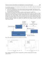
Fig. 4. Controlled outputs of the HEN system using (—) distributed MPC and ( )
coordinated decentralized MPC.
Figures 4 and 5 show the dynamic responses of the HEN operating with a distributed MPC
and a coordinated decentralized MPC. The worse performance is observed during the ﬁrst and
second load changes, most notably on y
1
and y
3
. The reasons for this behavior can be found
by observing the manipulated variables. The ﬁrst fact to be noted is that under nominal
steady-state conditions, u
4

is completely closed and y
2
is controlled by u
5
(see Figures 5.b),
achieving the maximum energy recovery. Observe also that u
6
is inactive since no heating
service is necessary at this point. After the ﬁrst load change occurs, both control variables u
2
and u
3
fall rapidly (see Figures 5.a). Under this conditions, the system activates the heater
ﬂow rate u
6
(see Figures 5.b). The dynamic reaction of the heater to the cool disturbance is
81
Distributed Model Predictive Control Based on Dynamic Games
18 Will-be-set-by-IN-TECH
also stimulated by u
2
, while u
6
takes complete control of y
1
, achieving the maximum energy
recovery. After the initial effect is compensated, y
3
is controlled through u
2

–which never
saturates–, while u
6
takes complete control of y
1
. Furthermore, Figure 5.b show that the cool
perturbation also affects y
2
,whereu
5
is effectively taken out of operation by u
4
.Theensuing
pair of load changes are heat perturbations featuring manipulated movements in the opposite
sense to those indicated above. Though the input change in h
2
allows returning the control of
y
1
from u
6
to u
3
(see Figures 5.a).
(a) u
1
( t), u
2
( t), u
3

( t) (b) u
4
( t), u
5
( t), u
6
( t)
Fig. 5. Manipulated inputs of the HEN system using (—) distributed MPC and ( )
coordinated decentralized MPC.
In these ﬁgures we can also see that the coordinated decentralized MPC fails to reject the ﬁrst
and second disturbances on y
1
and y
3
(see Figures 4.a and c) because it is not able to properly
coordinate the use of utility service u
6
to compensate the effects of active constraints on u
2
and
u
3
. This happens because the coordinated decentralized MPC is only able to address the effect
of interactions between agents but it can not coordinate the use of utility streams s
2
and s
3
to
avoid the output-unreachability under input constraint problem. The origin of the problem lies
in the cost function employed by the coordinated decentralized MPC, which does not include

the effect of the local decision variables on the other agents. This fact leads to different
steady–state values in the manipulated variables to those ones obtained by the distributed MPC
along the simulation.
Figure 6 shows the steady–state value of the recovered energy and utility services used by the
system for the distributed MPC schemes. As mentioned earlier, the centralized and distributed
MPC algorithms have similar steady–state conditions. These solutions are Pareto optimal,
hence they achieve the best plant wide performance for the combined performance index.
On the other hand, the coordinated decentralized MPC exhibited a good performance in energy
terms, since it employs less service energy, however it is not able of achieving the control
objectives, because it is not able of properly coordinate the use of utility ﬂows u
5
and u
6
.As
it was pointed out in previous Sections, the fact that the agents achieve the Nash equilibrium
does not implies the optimality of the solution.
Figure 7 shows the CPU time employed for each MPC algorithm during the simulations. As
it was expected, the centralized MPC is the algorithm that used more intensively the CPU.
Its CPU time is always larger than the others along the simulation. This fact is originated
on the size of the optimization problem and the dynamic of the system, which forces the
82
Advanced Model Predictive Control
Distributed Model Predictive Control
BasedonDynamicGames 19
Fig. 6. Steady-state conditions achieved by the HEN system for different MPC schemes.
Fig. 7. CPU times for different MPC schemes.
83
Distributed Model Predictive Control Based on Dynamic Games
20 Will-be-set-by-IN-TECH
centralized MPC to permanently correct the manipulated variable along the simulation due to

the system interactions. On the other hand, the coordinated decentralized MPC used the CPU
less intensively than the others algorithms, because of the size of the optimization problem.
However, its CPU time remains almost constant during the entire simulation since it needs to
compensate the interactions that had not been taken into account during the computation.
In general, all algorithms show larger CPU times after the load changes because of the
recalculation of the control law. However, we have to point out that the value of these peak
are smaller than sampling time.
6. Conclusions
In this work a distributed model predictive control framework based on dynamic games is
presented. The MPC is implemented in distributed way with the inexpensive agents within
the network environment. These agents can cooperate and communicate each other to achieve
the objective of the whole system. Coupling effects among the agents are taken into account
in this scheme, which is superior to other traditional decentralized control methods. The
main advantage of this scheme is that the on-line optimization can be converted to that
of several small-scale systems, thus can signiﬁcantly reduce the computational complexity
while keeping satisfactory performance. Furthermore, the design parameters for each agent
such as prediction horizon, control horizon, weighting matrix and sample time, etc. can
all be designed and tuned separately, which provides more ﬂexibility for the analysis and
applications. The second part of this study is to investigate the convergence, stability,
feasibility and performance of the distributed control scheme. These will provide users better
understanding to the developed algorithm and sensible guidance in applications.
7. Acknowledgements
The authors wishes to thank: the Agencia Nacional de Promoción Cientíﬁca y Tecnológica,the
Universidad Nacional de Litoral and the Consejo Nacional de Investigaciones Cientíﬁcas y Técnicas
(CONICET) from Argentina, for their support.
8. Appendices
A. Proof of Lemma 1
Proof. From deﬁnition of the J(·) we have
J
(

x(k) , U
q
(k), A
)
=
J

x(k) ,

U
q
j
∈N
1
(k) ···U
q
j
∈N
m
(k)

, A

(29)
From deﬁnition of U
q
j
∈N
l
.we have

J
(
x(k) , U
q
(k), A
)
=
J

x(k) ,

α
j∈N
1
˜
U
q
1
(k)+

1
− α
j∈N
1

U
q −1
j
∈N
1

(k) ···
α
j∈N
m
˜
U
q
j
∈N
m
(k)+

1
− α
j∈N
m

U
q −1
j
∈N
m
(k)

, A

=J

x(k) ,


α
j∈N
1

˜
U
q
j
∈N
1
(k) ···U
q −1
j
∈N
m
(k)

···
α
j∈N
m

U
q −1
j
∈N
1
(k) ···
˜
U

q
j
∈N
m
(k)

, A

84
Advanced Model Predictive Control
Distributed Model Predictive Control
BasedonDynamicGames 21
By convexity of J(·) we have
J
(
x(k) , U
q
(k), A
)
≤
m
∑
l=1
α
l
J

x(k) ,
˜
U

q
j
∈N
l
(k), U
q −1
j
∈I−N
l
(k), A

(30)
and from Algorithm 1 we know that
J

x
(k),
˜
U
q
j
∈N
l
(k), U
q −1
j
∈I−N
l
(k), A


≤ J

x(k) , U
q −1
(k), A

,
then
J
(
x(k) , U
q
(k), A
)
≤
J

x(k) ,
˜
U
q
j
∈N
l
(k), U
q −1
j
∈I−N
l
(k), A


≤ J

x(k) , U
q −1
(k), A

. (31)
Subtracting the cost functions at q
− 1andq we obtain
ΔJ

x
(k), U
q −1
(k), A

≤−ΔU
q −1
j
∈N
l
(k)
T
R ΔU
q −1
j
∈N
l
(k).

This shows that the sequence of cost

J
q
l
(k)

is non-increasing and the cost is bounded below
by zero and thus has a non-negative limit. Therefore as q
→ ∞ the difference of cost ΔJ
q
(k) →
0suchthattheJ
q
(k) → J
∗
(k).BecauseR > 0, as ΔJ
q
(k) → 0 the updates of the inputs
ΔU
q −1
(k) → 0asq → ∞, and the solution of the optimisation problem U
q
(k) converges to a
solution
¯
U
(k). Depending on the cost function employed by the distributed controllers,
¯
U(k)

can converge to U
∗
(k) (see Section 3.1).
B. Proof of Theorem 1
Proof. First it is shown that the input and the true plant state converge to the origin, and then
it will be shown that the origin is an stable equilibrium point for the closed-loop system. The
combination of convergence and stability gives asymptotic stability.
Convergence. Convergence of the state and input to the origin can be established by showing
that the sequence of cost values is non-increasing.
Showing stability of the closed-loop system follows standard arguments for the most part
Mayne et al. (2000), Primbs & Nevistic (2000). In the following, we describe only the most
important part for brevity, which considers the nonincreasing property of the value function.
The proof in this section is closely related to the stability proof of the FC-MPC method in
Venkat et al. (2008).
Let q
(k) and q(k + 1) stand for iteration number of Algorithm 1 at time k and k + 1respectively.
Let J
(k)=J
(
x(k) , U(k), A
)
and J(k + 1)=J
(
x(k + 1), U(k + 1), A
)
denote the cost value
associated with the ﬁnal combined solution at time k and k
+ 1. At time k + 1, let J
l
(k +

1)=J

x(k + 1), U
q
j
∈N
l
(k), U
q −1
j
∈I−N
l
(k), A

denote the global cost associated with solution of
subsystem l at iterate q.
The global cost function J
(
x(k) , U(k)
)
can be used as a Lyapunov function of the system, and
its non-increasing property can be shown following the chain
J
(
x(k + 1), U(k + 1), A
)
≤···≤
J
(
x(k + 1), U

q
(k + 1), A
)
≤···
···≤
J

x(k + 1), U
1
(k + 1), A

≤ J
(
x(k) , U(k), A
)
−
x(k)
T
Qx(k) − u(k)
T
Ru( k)
85
Distributed Model Predictive Control Based on Dynamic Games
22 Will-be-set-by-IN-TECH
The inequality J
(
x(k + 1), U
q
(k + 1), A
)

≤
J

x(k + 1), U
q −1+
(k + 1), A

is consequence of
Lemma 1. Using this inequality we can trace back to q
= 1
J
(
x(k + 1), U(k + 1), A
)
≤···≤
J
(
x(k + 1), U
q
(k + 1), A
)
≤···
···≤
J

x(k + 1), U
1
(k + 1), A

.

At time step q
= 1, we can recall the initial feasible solution U
0
(k + 1). At this iteration,
the distributed MPC optimizes the cost function with respect the local variables starting from
U
0
(k + 1), therefore ∀l = 1, ,m
J

x
(k + 1), U
1
j
∈N
l
(k), U
0
j
∈I−N
l
(k), A

≤ J

x(k + 1), U
0
(k), A

≤

∞
∑
i=1
x(k + i, k
T
Qx(k + i, k)+u(k + i, k)
T
Ru( k + i, k)
≤
J
(
x(k) , U(k), A
)
−
x(k)
T
Qx(k) − u(k)
T
Ru( k)
Due to the convexity of J and the convex combination up date (Step 2.c of Algorithm 1), we
obtain
J

x
(k), U
1
(k), A

≤
m

∑
l=1
α
l
J

x(k + 1), U
1
j
∈N
l
(k), U
0
j
∈I−N
l
(k), A

(32)
then,
J

x
(k), U
1
(k), A

≤
m
∑

l=1
α
l

J
(
x(k) , U(k), A
)
−
x(k)
T
Qx(k) − u(k)
T
Ru( k)

,
≤ J
(
x(k) , U(k), A
)
−
x(k)
T
Qx(k) − u(k)
T
Ru( k).
Subtracting J
∗
(k) from J
∗

(k + 1)
J
∗
(k + 1) − J
∗
(k) ≤−x(k)
T
Qx(k) − u(k)
T
Ru( k) ∀k. (33)
This shows that the sequence of optimal cost values
{
J
∗
(k)
}
decreases along closed-loop
trajectories of the system. The cost is bounded below by zero and thus has a non–negative
limit. Therefore as k
→ ∞ the difference of optimal cost ΔJ
∗
(k + 1) → 0. Because Q and R
are positive deﬁnite, as ΔJ
∗
(k + 1) → 0 the states and the inputs must converge to the origin
x
(k) → 0andu(k) → 0ask → ∞.
Stability. Using the QP form of (6), the feasible cost at time k
= 0 can be written as follows
J

(0)=x(0)
T
¯
Qx
(0),where
¯
Q is the solution of the Lyapunov function for dynamic matrix
¯
Q
= A
T
QA + Q.
From equation (33) it is clear that the sequence of optimal costs
{
J
∗
(k)
}
is non-increasing,
which implies J
∗
(k) ≤ J
∗
(0) ∀k > 0. From the deﬁnition of the cost function it follows that
x
T
(k)Qx(k) ≤ J
∗
(k) ∀k, which implies
x

T
(k)Qx(k) ≤ x(0)
T
¯
Qx
(0) ∀k.
Since Q and
¯
Q are positive deﬁnite it follows that

x(k)

≤ γ

x(0)

∀k > 0
86
Advanced Model Predictive Control
Distributed Model Predictive Control
BasedonDynamicGames 23
where
γ
=

λ
max
(
¯
Q

)
λ
min
(Q)
.
Thus, the closed-loop is stable. The combination of convergence and stability implies that the
origin is asymptotically stable equilibrium point of the closed-loop system.
C. Proof of Theorem 2
Proof. The optimal solution of the distributed control system with communications faults is
given by
˜
U
(k)=
(
I −K
0
RCT
)
−1
K
1
RCT Γx(k). (34)
Using the matrix decomposition technique, it gives
(
I −K
0
RCT
)
−1
=

(
I −K
0
)
−1

2I
−

I
+
(
I −K
0
)
−1
(
I + K
0
− 2K
0
RCT
)]
−1

+
(
I −K
0
)

−1
In general
(
I −K
0
)
−1
and
(
I + K
0
− 2K
0
RCT
)
−1
all exist, therefore the above equation
holds. Now, from (34) we have
K
1
Γx(k)=
(
I −K
0
)
U(k),then
˜
U(k) canbewrittenasa
function of the optimal solution U
(k) as follows

˜
U
(k)=
(
S + I
)
U(k)
where S = 2I −

I
+
(
I −K
0
)
−1
(
I + K
0
− 2K
0
RCT
)

−1
.
The cost function of the system free of communication faults J
∗
can be written as function of
U

(k) as follows
J
∗
=



K
−1
1
(
I −K
0
)
U(k) −HU(k)



2
Q
+

U(k)

2
R
=

U(k)


2
F
(35)
where
F =

K
−1
1
(
I −K
0
)
−H

T
Q

K
−1
1
(
I −K
0
)
−H

+ R.
In the case of the system with communication failures we have
˜

J
≤ J
∗
+

U(k)

2
W
(36)
where
W = S
T

H
T
QH + R

S. Finally, the effect of communication can be related with J
∗
through

U(k)

2
W
≤

W


λ
min
(F )
J
∗
, (37)
where λ
min
denotes the minimal eigenvalue of F. From the above derivations, the relationship
between
˜
J and J
∗
is given by
˜
J
≤

1
+

W

λ
min
(F )

J
∗
. (38)

and the degradation is
˜
J
− J
∗
J
∗
≤

W

λ
min
(F )
. (39)
87
Distributed Model Predictive Control Based on Dynamic Games
24 Will-be-set-by-IN-TECH
Inspection of (36) shows that

W

depends on R and T . So in case of all communication
failures existed,

W

can arrive at the maximal value
W
max

=

2I
−

I
+
(
I −K
0
)
−1
(
I + K
0
)

−1

T

H
T
QH + R


2I
−

I

+
(
I −K
0
)
−1
(
I + K
0
)

−1

,
and the upper bound of performance deviation is
˜
J
− J
∗
J
∗
≤

W
max

λ
min
(F )
. (40)

9. References
Aguilera, N. & Marchetti, J. (1998). Optimizing and controlling the operation of heat
exchanger networks, AIChe Journal 44(5): 1090–1104.
Aske, E., Strand, S. & Skogestad, S. (2008). Coordinator mpc for maximizing plant throughput,
Computers and Chemical Engineering 32(1-2): 195–204.
Bade, S., Haeringer, G. & Renou, L. (2007). More strategies, more nash equilibria, Journal of
Economic Theory 135(1): 551–557.
Balderud, J., Giovanini, L. & Katebi, R. (2008). Distributed control of underwater vehicles,
Proceedings of the Institution of Mechanical Engineers, Part M: Journal of Engineering for
the Maritime Environment 222(2): 95–107.
Bemporad, A., Filippi, C. & Torrisi, F. (2004). Inner and outer approximations of polytopes
using boxes, Computational Geometry: Theory and Applications 27(2): 151–178.
Bemporad, A. & Morari, M. (1999). Robust model predictive control: A survey, in
robustness in identiﬁcation and control, Lecture Notes in Control and Information
Sciences 245: 207–226.
Braun, M., Rivera, D., Flores, M., Carlyle, W. & Kempf, K. (2003). A model predictive
control framework for robust management of multi-product, multi-echelon demand
networks, Annual Reviews in Control 27(2): 229–245.
Camacho, E. & Bordons, C. (2004). Model predictive control,Springer.
Camponogara, E., Jia, D., Krogh, B. & Talukdar, S. (2002). Distributed model predictive
control, IEEE Control Systems Magazine 22(1): 44–52.
Cheng, R., Forbes, J. & Yip, W. (2007). Price-driven coordination method for solving
plant-wide mpc problems, Journal of Process Control 17(5): 429–438.
Cheng, R., Fraser Forbes, J. & Yip, W. (2008). Dantzig–wolfe decomposition and plant-wide
mpc coordination, Computers and Chemical Engineering 32(7): 1507–1522.
Dubey, P. & Rogawski, J. (1990). Inefﬁciency of smooth market mechanisms, Journal of
Mathematical Economics 19(3): 285–304.
Dunbar, W. (2007). Distributed receding horizon control of dynamically coupled nonlinear
systems, IEEE Transactions on Automatic Control 52(7): 1249–1263.
Dunbar, W. & Murray, R. (2006). Distributed receding horizon control for multi-vehicle

formation stabilization, Automatica 42(4): 549–558.
88
Advanced Model Predictive Control
Distributed Model Predictive Control
BasedonDynamicGames 25
Goodwin, G., Salgado, M. & Silva, E. (2005). Time-domain performance limitations arising
from decentralized architectures and their relationship to the rga, International Journal
of Control 78(13): 1045–1062.
Haimes, Y. & Chankong, V. (1983). Multiobjective decision making: Theory and methodology,North
Holland, New York.
Henten, E. V. & Bontsema, J. (2009). Time-scale decomposition of an optimal control problem
in greenhouse climate management, Control Engineering Practice 17(1): 88–96.
Hovd, M. & Skogestad, S. (1994). Sequential design of decentralized controllers, Automatica
30: 1601–1601.
Jamoom, M., Feron, E. & McConley, M. (2002). Optimal distributed actuator control grouping
schemes, Proceedings of the 37th IEEE Conference on Decision and Control,Vol.2,
pp. 1900–1905.
Jia, D. & Krogh, B. (2001). Distributed model predictive control, American Control Conference,
2001. Proceedings of the 2001,Vol.4.
Jia, D. & Krogh, B. (2002). Min-max feedback model predictive control for distributed control
with communication, American Control Conference, 2002. Proceedings of the 2002,Vol.6.
Kouvaritakis, B. & Cannon, M. (2001). Nonlinear pr edictive control: theory and practice,Iet.
Kumar, A. & Daoutidis, P. (2002). Nonlinear dynamics and control of process systems with
recycle, Journal of Process Control 12(4): 475–484.
Lu, J. (2003). Challenging control problems and emerging technologies in enterprise
optimization, Control Engineering Practice 11(8): 847–858.
Maciejowski, J. (2002). Predictive control: with constraints, Prentice Hall.
Mayne, D., Rawlings, J., Rao, C. & Scokaert, P. (2000). Constrained model predictive control:
Stability and optimality, Automatica 36: 789–814.
Motee, N. & Sayyar-Rodsari, B. (2003). Optimal partitioning in distributed model predictive

control, Proceedings of the American Control Conference, Vol. 6, pp. 5300–5305.
Nash, J. (1951). Non-cooperative games, Annals of mathematics pp. 286–295.
Neck, R. & Dockner, E. (1987). Conﬂict and cooperation in a model of stabilization policies: A
differential game approach, J. Econ. Dyn. Cont 11: 153–158.
Osborne, M. & Rubinstein, A. (1994). A course in game theory, MIT press.
Perea-Lopez, E., Ydstie, B. & Grossmann, I. (2003). A model predictive control strategy for
supply chain optimization, Computers and Chemical Engineering 27(8-9): 1201–1218.
Primbs, J. & Nevistic, V. (2000). Feasibility and stability of constrained ﬁnite receding horizon
control, Automatica 36(7): 965–971.
Rossiter, J. (2003). Model-based predictive control: a practical approach, CRC press.
Salgado, M. & Conley, A. (2004). Mimo interaction measure and controller structure selection,
International Journal of Control 77(4): 367–383.
Sandell Jr, N., Varaiya, P., Athans, M. & Safonov, M. (1978). Survey of decentralized
control methods for large scale systems, IEEE Transactions on Automatic Control
23(2): 108–128.
Vaccarini, M., Longhi, S. & Katebi, M. (2009). Unconstrained networked decentralized model
predictive control, Journal of Process Control 19(2): 328–339.
Venkat, A., Hiskens, I., Rawlings, J. & Wright, S. (2008). Distributed mpc strategies with
application to power system automatic generation control, IEEE Transactions on
Control Systems Technology 16(6): 1192–1206.
Šiljak, D. (1996). Decentralized control and computations: status and prospects, Annual
Reviews in Control 20: 131–141.
89
Distributed Model Predictive Control Based on Dynamic Games
26 Will-be-set-by-IN-TECH
Wittenmark, B. & Salgado, M. (2002). Hankel-norm based interaction measure for
input-output pairing, Proc. of the 2002 IFAC World Congress.
Zhang, Y. & Li, S. (2007). Networked model predictive control based on neighbourhood
optimization for serially connected large-scale processes, Journal of process control
17(1): 37–50.

Zhu, G. & Henson, M. (2002). Model predictive control of interconnected linear and nonlinear
processes, Industrial and Engineering Chemistry Research 41(4): 801–816.
90
Advanced Model Predictive Control
5
Efficient Nonlinear Model Predictive
Control for Affine System
Tao ZHENG and Wei CHEN
Hefei University of Technology
China
1. Introduction
Model predictive control (MPC) refers to the class of computer control algorithms in which a
dynamic process model is used to predict and optimize process performance. Since its lower
request of modeling accuracy and robustness to complicated process plants, MPC for linear
systems has been widely accepted in the process industry and many other fields. But for
highly nonlinear processes, or for some moderately nonlinear processes with large operating
regions, linear MPC is often inefficient. To solve these difficulties, nonlinear model
predictive control (NMPC) attracted increasing attention over the past decade (Qin et al.,
2003, Cannon, 2004). Nowadays, the research on NMPC mainly focuses on its theoretical
characters, such as stability, robustness and so on, while the computational method of
NMPC is ignored in some extent. The fact mentioned above is one of the most serious
reasons that obstruct the practical implementations of NMPC.
Analyzing the computational problem of NMPC, the direct incorporation of a nonlinear
process into the linear MPC formulation structure may result in a non-convex nonlinear
programming problem, which needs to be solved under strict sampling time constraints and
has been proved as an NP-hard problem (Zheng, 1997). In general, since there is no accurate
analytical solution to most kinds of nonlinear programming problem, we usually have to
use numerical methods such as Sequential Quadric Programming (SQP) (Ferreau et al., 2006)
or Genetic Algorithm (GA) (Yuzgec et al., 2006). Moreover, the computational load of NMPC
using numerical methods is also much heavier than that of linear MPC, and it would even

increase exponentially when the predictive horizon length increases. All of these facts lead
us to develop a novel NMPC with analytical solution and little computational load in this
chapter.
Since affine nonlinear system can represents a lot of practical plants in industry control,
including the water-tank system that we used to carry out the simulations and experiments,
it has been chosen for propose our novel NMPC algorithm. Follow the steps of research
work, the chapter is arranged as follows:
In Section 2, analytical one-step NMPC for affine nonlinear system will be introduced at first,
then, after description of the control problem of a water-tank system, simulations will be
carried out to verify the result of theoretical research. Error analysis and feedback
compensation will be discussed with theoretical analysis, simulations and experiment at last.
Then, in Section 3, by substituting reference trajectory for predicted state with stair-like
control strategy, and using sequential one-step predictions instead of the multi-step

Advanced Model Predictive Control

92
prediction, the analytical multi-step NMPC for affine nonlinear system will be proposed.
Simulative and experimental control results will also indicate the efficiency of it. The
feedback compensation mentioned in Section 2 is also used to guarantee the robustness to
model mismatch.
Conclusion and further research direction will be given at last in Section 4.
2. One-step NMPC for affine system
2.1 Description of NMPC for affine system
Consider a time-invariant, discrete, affine nonlinear system with integer k representing the
current discrete time event:

k+1 k k k k
x =f(x )+g(x )×u +ξ (1a)
s. t.

n
k
xXR (1b)

m
k
uUR (1c)

n
k
ξ R
(1d)
In the above,
kkk
u,x,ξ are input, state and disturbance of the system respectively,
nn
f:R R ,
nn×m
g:R R are corresponding nonlinear mapping functions with proper
dimension.
Assume
k+
j
|k
ˆ
x are predictive values of
k+
j
x at time k,
kkk-1

Δu=u-u
and
k+
j
|k
ˆ
Δuare the
solutions of future increment of
k+
j
u at time k, then the objective function
k
J
can be written
as follow:

p-1
k k+p|k k+
j
|k k+
j
|k
j=0
ˆˆ
J=F(x )+ G(x ,Δu)

(2)
The function F (.) and G (. , .) represent the terminal state penalty and the stage cost
respectively, where p is the predictive horizon.
In general,

k
J usually has a quadratic form. Assume
k+
j
|k
w
is the reference value of
k
j
x

at
time k which is called reference trajectory (the form of
k
j
|k
w

will be introduced with detail
in Section 2.2 and 3.1 for one-step NMPC and multi-step NMPC respectively), semi-positive
definite matrix Q and positive definite matrix R are weighting matrices, (2) now can be
written as :

pp1
22
k k j|k k j| k k j| k
QR
j1 j0
ˆ
Jxw u


 



(3)
Corresponding to (1) and (3), the NMPC for affine system at each sampling time now is
formulated as the minimization of
k
J , by choosing the increments sequence of future
control input
k| k k 1| k k p 1|k
[u u u ]

  , under constraints (1b) and (1c).

Efficient Nonlinear Model Predictive Control for Affine System

93
By the way, for simplicity, In (3), part of
k
J is about the system state
k
x , if the output of the
system
kk
y
Cx , which is a linear combination of the state (C is a linear matrix), we can
rewrite (3) as follow to make an objective function
k

J about system output:

pp1
22
k k j| k k j| k k j| k
QR
j1 j0
ˆ
JCxw u

 



pp1
22
kj|k kj|k kj|k
QR
j1 j0
ˆ
yw u

 



(4)
And sometimes,
k
j

|k
u


in
k
J could also be changed as
k
j
|k
u

to meet the need of practical
control problems.
2.2 One-step NMPC for affine system
Except for some special model, such as Hammerstein model, analytic solution of multi-step
NMPC could not be obtained for most nonlinear systems, including the NMPC for affine
system mentioned above in Section 2.1. But if the analytic inverse of system function exists
(could be either state-space model or input-state model), the one-step NMPC always has the
analytic solution. So all the research in this chapter is not only suitable for affine nonlinear
system, but also suitable for other nonlinear systems, that have analytic inverse system
function.
Consider system described by (1a-1d) again, the one-step prediction can be deduced directly
as follow with only one unknown data
k| k k| k k 1
uuu


 at time k:

 



.
Especially, if
k
 is a stationary stochastic noise with zero mean and variance
2
k
E[ ], it is
easy known that
k1|k
E[x ] 0



, and
T2
k1|k k1|k k1|k k1|k
E[(x E[x ]) (x E[x ])] n
 

 
 
, in
another word, both the mean and the variance of the predictive error have a minimum
value, so the prediction is an optimal prediction here in (5).
Then if the setpoint is
sp

x , and to soften the future state curve, the expected state value at
time k+1 is chosen as
k1|k k sp
wx(1)x


 , where
[0,1)
is called soften factor, thus
the objective function of one-step NMPC can be written as follow:

22
kk1|kk1|k k|k
QR
ˆ
Jx w u

  (6)
To minimize
k
J without constraints (1b) and (1c), we just need to have
k
k| k
J
0
u



and

2
k
2
k| k
J
0
u



, then:

T11
k| k k k k k 1|k k 1| k
ˆ
u(
g
(x ) Q
g
(x ) R) (
g
(x ) Q (x w ))


     (7)

Advanced Model Predictive Control

94
Mark

T
kk
Hg(x)Qg(x)R and
1
k k 1| k k 1| k
ˆ
F
g
(x ) Q (w x )

  , so the increment of
instant future input is:

1
k| k
uHF

 (8)
But in practical control problem, limitations on input and output always exist, so the result
of (8) is usually not efficient. To satisfy the constraints, we can just put logical limitation on
amplitudes of
k
u and
k
x , or some classical methods such as Lagrange method could be
used. For simplicity, we only discuss about the Lagrange method here in this chapter.
First, suppose every constraint in (1b) and (1c) could be rewritten in the form as
T
ik|k i
au b, i1,2,q  , then the matrix form of all constraints is:

k|k
Au B

 (9)
In which,
T
TT T
12 q
Aaa a



T
12 q
Bbb b





.
Choose Lagrange function as
TT
ki k i i k|k i
L( ) J (a u b)   
, i1,2,q

 , let
k| k i i

k| k
L
Hu F a 0
u

 

and
T
ik|ki
i
L
au b 0




, then:

1
k| k i i
uH(Fa)


  
(10a)

T1
ii
i

T1
ii
aH F b
aH a



 (10b)
If
i
0
in (10b), means that the corresponding constraint has no effect on
k|k
u

, we can
choose
i
0 , but if
i
0


in (10b), the corresponding constraint has effect on
k
u
indeed,
so we must choose
ii


 , finally, the solution of one-step NMPC with constraints could
be:

1T
k| k
uH(FA)


   (11)
In which,
T
12 q

   


2.3 Control problem of the water-tank system
Our plant of simulations and experiments in this chapter is a water-tank control system as
that in Fig. 1. and Fig. 2. (We just used one water-tank of this three-tank system). Its affine
nonlinear model is achieved by mechanism modeling (Chen
et al., 2006), in which the
variables are normalized, and the sample time is 1 second here:

k1 k k k
x x 0.2021 x 0.01923u

 
(12a)
s. t.
k

x [0%,100%]

(12b)

Efficient Nonlinear Model Predictive Control for Affine System

95

k
u [0%,100%]

(12c)
In (12),
k
x is the height of water in the tank, and
k
u is the velocity of water flow into the
tank, from pump P
1
and valve V
1
, while valve V
2
is always open. In the control problem of
the water-tank, for convenience, we choose the system state as the output, that means
kk
y
x
, and the system functions are
kk k

f(x ) x 0.2021 x and
k
g
(x ) 0.01923
.

Fig. 1. Photo of the water-tank system

Fig. 2. Structure of the water-tank system
To change the height of the water level, we can change the velocity of input flow, by
adjusting control current of valve V
1,
and the normalized relation between the control
current and the velocity
k
u is shown in Fig. 3.

Advanced Model Predictive Control

96
0% 25% 50% 75% 100%
0%
20%
40%
60%
80%
100%
control current

u

Fig. 3. The relation between control current and input
k
u
2.4 One-step NMPC of the water-tank system and its feedback compensation
Choose objective function
22
kk1|kk1|k k|k
ˆ
J (x w ) 0.001 u

 ,
sp
x 30%

and soften
factor 0.95 , to carry out all the simulations and the experiment in this section. (except for
part of Table 1., where we choose 0.975

 )
Suppose there is no model mismatch, the simulative control result of one-step NMPC for
water-tank system is obtained as Fig. 4. and it is surely meet the control objective.

0 50 100 150
10%
20%
30%
40%
x

0 50 100 150
40%
50%
60%
70%
80%
u
time(sec)

Fig. 4. Simulation of one-step NMPC without model mismatch and feedback compensation
To imitate the model mismatch, we change the simulative model of the plant from
k1 k k k
x x 0.2021 x 0.01923u

 
to
k1 k k k
x x 110% 0.2021 x 90% 0.01923u

   
, but
still use
k1 k k k
x x 0.2021 x 0.01923u

  to be the predictive model in one-step NMPC,
the result in Fig. 5. now indicates that there is obvious steady-state error.

Efficient Nonlinear Model Predictive Control for Affine System

97
0 50 100 150
10%
20%
30%
40%
x
0 50 100 150
40%
50%
60%
70%
80%
u
time(sec)

Fig. 5. Simulation of one-step NMPC with model mismatch but without feedback
compensation
Proposition 1: For affine nonlinear system
k1 k k k
xf(x)
g
(x ) u




, if the setpoint is
sp
x,

steady-state is
s
u and
s
x , and the predictive model is
k1 k k k
xf(x)
g
(x ) u


, without
consideration of constraints, the steady-state error of one-step NMPC is
ss s ss
ssp
(f (x ) f(x )) (
g
(x )
g
(x )) u
ex x
1



 

, in which

is the soften factor.

Proof: If the system is at the steady-state, then we have
k1 k s
xxx


 and
k1 k s
uuu

.
Since
k1 k s
uuu

, so
k
u0

 , from (8), we know matrix F=0, or equally
1
k1|k k1|k
ˆ
(w x ) 0


.
Update the process of one-step NMPC at time k, we have:

k1|k k sp s sp
wx(1)xx(1)x



  (13)

1
k1|k k k k1 s s s
ˆ
xf(x)
g
(x ) u f(x )
g
(x ) u



(14)
(13)-(14), and notice that
ss ss
xf(x)
g
(x ) u




for steady-state, we get:
0
s sp s sss s ss sp s
x(1 )x f(x)
g

(x ) u x f(x )
g
(x ) u (1 )x (1 )x         
ss s ss sps
(f (x ) f(x )) (
g
(x )
g
(x )) u (1 ) (x x )



 
So:

ss s ss
ssp
(f (x ) f(x )) (
g
(x )
g
(x )) u
ex x
1



 

(15)

Proof end.
Because the soften factor
[0,1)

 , thus 1 0

 always holds, the necessary condition for
e0 is
ss s ss
(f (x ) f(x )) (
g
(x )
g
(x )) u 0

 . When there is model mismatch, there will be
steady-state error, while this error is independent of weight matrix Q and dependent of the

Advanced Model Predictive Control

98
soften factor  . For corresponding discussion on steady-state error of one-step NMPC with
constraints, the only difference is (11) will take the place of (8) in the proof.
Table 1. is the comparison on
ssp
ex x

 between simulation and theoretical analysis, and
they have the same result. (simulative model
k1 k k k

x x 110% 0.2021 x 90% 0.01923u

    ,
predictive model
k1 k k k
x x 0.2021 x 0.01923u

  )



Q

ssp
ex x


Simulation(%)
ssp
ex x


Value of (15)(%)
0.975
0 -8.3489 -8.3489
0.001 -8.3489 -8.3489
0.01 -8.3489 -8.3489
0.95

0 -4.5279 -4.5279

0.001 -4.5279 -4.5279
0.01 -4.5279 -4.5279
Table 1. Comparison on
ssp
ex x

 between simulation and theoretical analysis
From (15) we know, we cannot eliminate this steady-state error by adjusting

, so feedback
compensation could be used here, mark the predictive error
k
e at time k as follow:

1
kkk|k1k k|k1 k1 k1
ˆˆ
exx x(x
g
(x ) u )

   
(16)
In which,
k
x is obtained by system feedback at time k, and
k|k 1
ˆ
x


is the predictive value of
k
x at time k-1.
Then add
k
e to the predictive value of
k1
x

at time k directly, so (5) is rewritten as follow:

1
k 1|k k k k 1 k k |k k k 1|k k k|k k
ˆˆ
xf(x)
g
(x ) u
g
(x ) u e x
g
(x ) u e
 

 
(17)
Use this new predictive value to carry out one-step NMPC, the simulation result in Fig. 6.
verify its robustness under model mismatch, since there is no steady-state error with this
feedback compensation method.
The direct feedback compensation method above is easy to understand and carry out, but it
is very sensitive to noise. Fig. 7. is the simulative result of it when there is noise add to the

system state, we can see that the input vibrates so violently, that is not only harmful to the
actuator in practical control system, but also harmful to system performance, because the
actuator usually cannot always follow the input signal of this kind.
To develop the character of feedback compensation, simply, we can use the weighted
average error
k
e
instead of single
k
e
in (17):

s
1
k 1|k k 1|k k k|k i k 1 i
i1
ˆˆ
xxg(x)u he
 



1
k1|k k k|k k
ˆ
x
g
(x ) u e



,
s
i
i1
h1



(18)
Choose i 20
 ,
i
h0.05

, the simulative result is shown in Fig. 8. Compared with Fig. 7. it
has almost the same control performance, but the input is much more smooth now. Using
the same method and parameters, experiment has been done on the water-tank system, the
result in Fig. 9. also verifies the efficiency of the proposed one-step NMPC for affine systems
with feedback compensation.

Efficient Nonlinear Model Predictive Control for Affine System

99

0 50 100 150
10%
20%
30%
40%
x
0 50 100 150
40%
60%
80%
100%
u
time(sec)

Fig. 6. Simulation of one-step NMPC with model mismatch and direct feedback compensation

0 50 100 150
10%
20%
30%
40%
x

0 50 100 150
40%
60%
80%
100%
u
time(sec)

Fig. 7. Simulation of one-step NMPC with model mismatch, noise and direct feedback
compensation

Advanced Model Predictive Control

100

40 60 80 100 120 140 160 180
10%
20%
30%
40%
x
40 60 80 100 120 140 160 180
40%
60%
80%
100%
u
time(sec)

Fig. 8. Simulation of one-step NMPC with model mismatch, noise and smoothed feedback
compensation

0 50 100 150 200
10%
20%
30%
40%
x
0 20 40 60 80 100 120 140 160 180 200
30%
40%
50%
60%
time (sec)
control current
0 20 40 60 80 100 120 140 160 180 200
40%
60%
80%
100%
u

Fig. 9. Experiment of one-step NMPC with setpoint
sp

x 30%


Efficient Nonlinear Model Predictive Control for Affine System

101
3. Efficient multi-step NMPC for affine system
Since reference trajectory and stair-like control strategy will be used to establish efficient
multi-step NMPC for affine system in this chapter, we will introduce them in Section 3.1 and
3.2 at first, and then, the multi-step NMPC algorithm will be discussed with theoretical
research, simulations and experiments.
3.1 Reference trajectory for future state
In process control, the state usually meets the objective in the form of setpoint along a softer
trajectory, rather than reach the setpoint immediately in only one sample time. This may
because of the limit on control input, but a softer change of state is often more beneficial to
actuators, even the whole process in practice. This trajectory, usually called reference
trajectory, often can be defined as a first order exponential curve:

kj|k kj1|k sp
ww(1)x,j1,2,,p1


 
(19)
In which,
sp
x still denotes the setpoint, [0,1)

 is the soften factor, and the initial value of

the trajectory is
k| k k
wx

.The value of

determines the speed of dynamic response and
the curvature of the trajectory, the larger it is, the softer the curve is. Fig. 10. shows different
trajectory with different

. Generally speaking, suitable

could be chosen based on the
expected setting time in different practical cases.

0 50 100 150
0
setpoint
time
x
alfa=0
alfa=0.8
alfa=0.9
alfa=0.95

Fig. 10. Reference trajectory with different soften factor


3.2 Stair-like control strategy
To lighten the computational load of nonlinear optimization, which is one of the biggest obstacles

in NMPC’s application, stair-like control strategy

is introduced here. Suppose the first unknown
control input’s increment
kkk1
uuu


 , and the stair coefficient

is a positive real
number, then the future control input’s increment can be decided by the following expression:

jj
kj kj1 k
uu u,
j
1,2, ,p 1


       (20)

Advanced Model Predictive Control

102
Instead of the full future sequence of control input’s increment:
kk1 kp1
[u u u ]




 ,
which has p independent variables. Using this strategy, in multi-step NMPC, it now need
only compute
k
u . The computational load now is independent of the length of predictive
horizon, which is very convenient for us to choose long predictive horizon in NMPC to
obtain a better control performance (Zheng
et al., 2007).
Since the dynamic optimization process will be repeated at every sample time, and only
instant input
kk-1 k
uu u


will be carried out actually in NMPC, this strategy is efficient
here. In the strategy, it supposes the future increase of control input will be in a same
direction, which is the same as the experience in control practice of the human beings, and
prevents the frequent oscillation of the input, which is very harmful to the actuators in real
control plants. Fig. 11. shows the input sequences with different

.
3.3 Multi-step NMPC for affine system
The one-step NMPC in Section 2 is simple and fast, but it also has one fatal disadvantage.
Its predictive horizon is only one step, while long predictive horizon is usually needed for
better performance in MPC algorithms. One-step prediction may lead overshooting or other
bad influence on system’s behaviour. So we will try to establish a novel efficient multi-step
NMPC based on proposed one-step NMPC in this section.
In this multi-step NMPC algorithm, the first step prediction is the same as (5), then follows
the prediction of

k1|k
ˆ
x

in (5), the one-step prediction of
kj|k
ˆ
x,j2,3,,p


 could be
obtained directly:

0 1 2 3 4 5
0
2
4
6
8
10
12
14
16
time
u
beta=2

beta=1
beta=0.5

Fig. 11. Stair-like control strategy

Efficient Nonlinear Model Predictive Control for Affine System

103

k
j
|k k
j
1| k k
j
1| k k
j
1|k
ˆˆ ˆ
x f(x ) g(x ) u
 

 (21)
Since
k
j

1| k
ˆ
x

already contains nonlinear function of former data, one may not obtain the
analytic solution of (21) for prediction more than one step. Take the situation of j=2 for
example:

k 2|k k 1|k k 1|k k 1|k
ˆˆ ˆ
x f(x ) g(x ) u
 

kkk|k kkk|kk1|k
f(f(x ) g(x ) u ) g(f(x ) g(x ) u ) u


 (22)
For most nonlinear f(.) and g(.), the embedding form above makes it impossible to get an
analytic solution of
k1
u

and further future input. So, using reference trajectory, we
modified the one-step predictions when
j
2
as follow:

k

j
|k k
j
1| k k
j
1| k k
j
1
ˆ
xf(w)g(w)u
 

j1
k
j
1| k k
j
1|k k 1 k i |k
i0
f(w )
g
(w ) (u u )

   



(23)
Using the stair-like control strategy, mark
k|k

u

, (23) can be transformed as:
j1
i
kj|k kj1|k kj1|k k1
i0
ˆ
xf(w)
g
(w ) (u )

 





j1
i
kj1|k kj1|k k1 kj1|k
i0
f(w ) g(w ) u g(w )

   





j1
1i
kj|k kj1|k
i0
ˆ
xg(w)






(24)
Here,
1
k
j
|k
ˆ
x

contains only the known data at time k, while the other part is made up by the
increment of future input, thus the unknown data are separated linearly by (24), so the
analytic solution of

can be achieved.
For
j
1,2, ,p  , write the predictions in the form of matrix: