Advanced Model Predictive Control Part 11 pptx

Nonlinear Autoregressive with Exogenous Inputs
Based ModelPredictive Control for Batch Citronellyl Laurate Esterification Reactor
289
Eaton, J.W. and Rawlings, J.B. (1992) Model predictive control of chemical processes.
Chemical Engineering Science. 47, 705-720.
Foss, B.A., Johansen, T.A. and Sorensen, A.V. (1995). Nonlinear predictive control using
local models-applied to a batch fermentation process. Control Engineering Practice. 3
(3), 389-396.
Garcia, C.E. and Morari, M., (1982) Internal model control. 1. A Unifying review and some
new results, Ind Eng Chem Process Des Dev, 21: 308-323.
Garcia, T., Coteron, A., Martinez, M. and Aracil, J. (1996) Kinetic modelling for the
esterification reactions catalysed by immobilized lipases” Chemical Engineering
Science. 51, 2846-2846
Garcia, T., Sanchez, N., Martinez, M. and Aracil, J. (1999) Enzymatic synthesis of fatty esters-
Part I: Kinetic approach. Enzyme and Microbial Technology. 25, 584-590.
Garcia, T., Coteron, A., Martinez, M. and Aracil, J. (2000) Kinetic model for the esterification
of oleic acid and cetyl alcohol using immobilized lipase as catalyst. Chemical
Engineering Science. 55, 1411-1423
Garcia, R.M., Wornle, F., Stewart, B.G. and Harrison D.K. (2002) Real-Time remote network
control of an inverted pendulum using ST-RTL. Proceeding for 32nd ASEE/IEEE
Frontiers in Education Conference Boston. 18-23
Gattu, G. and Zafiriou, E. (1992) Nonlinear quadratic dynamic matrix control with state
estimation. Ind. Eng. Chem. Res., 31 (4), 1096-1104.
Harris, T.J. and Yu, W. (2007) Controller assessment for a class of nonlinear systems. Journal
of Process Control, 17: 607-619
Henson, M.A. (1998) Nonlinear model predictive control: Current status and future
directions. Computers and Chemical Engineering, 23, 187-202
Hua, X., Rohani, S., and Jutan, A. (2004). Cascade closed-loop optimization and control of
batch reactors. Chemical Engineering Sciencel 59, 5695-5708
Li, S., Lim, K.Y. and Fisher, D.G. (1989) A State Space Formulation for Model Predictive
Control. AIChe Journal. 35(2), 241-249.

Liu, Z.H. and Macchietto, S. (1995). Model based control of a multipurpose batch reactor.
Computers Chem. Engng 19, 477-482.
Mayne, D.Q., Rawlings, J.B., Rao, C.V. & Scokaert, P.O.M. (2000). Constrained model
predictive control: Stability and optimality. Automatica, 36, 789-814.
M’sahli, F., Abdennour, R. B. and Ksouri, M. (2002) Nonlinear Model-Based Predictive
Control Using a Generalised Hammerstein Model and its Application to a Semi-
Batch Reactor. International Journal Advanced Manufacturing Technology 20, 844–852.
Morari, M. & Lee, J.H. (1999) Model predictive control: Past, present and future, Computers
and Chemical Engineering, 23, 667-682
Mu, J., Rees, D. and Liu, G.P., 2005, Advanced controller design for aircraft gas turbine
engines. Control Engineering Practice, 13: 1001–1015
Nagy, Z.K., Mahn, B., Franke, R. and Allgower, F. (2007). Evaluation study of an efficient
output feedback nonlinear model predictive control for temperature tracking in an
industrial batch reactor. Control Engineering Practice 15, 839–850.

Advanced Model Predictive Control
290
Ozkan, G., Hapoglu, H. and Alpbaz, M. (2006). Non-linear generalised predictive control of
a jacketed well mixed tank as applied to a batch process- A polymerisation
reaction. Applied Thermal Engineering 26, 720–726.
Petersson, A.E.V., Gustafsson, L.M., Nordblad, M,, Boerjesson, P., Mattiasson, B., &
Adlercreutz, P. (2005) Wax esters produced by solvent-free energy efficient
enzymatic synthesis and their applicability as wood coatings. Green Chem. 7(12),
837–843.
Qin, S.J., T.A. Badgwell (2003). A survey of industrial model predictive control technology,
Control Engineering Practice, 11(7), 733-764.
Serri N.A., Kamaruddin

A.H., and Long

W.S. (2006). Studies of reaction parameters on
synthesis of Citronellyl laurate ester via immobilized Candida rugosa lipase in
organic media. Bioprocess and Biosystems Engineering 29, 253-260.
Shafiee, G., Arefi, A.A., Jahed-Motlagh, M.R. and Jalali, A.A. (2008) Nonlinear predictive
control of a polymerization reactor based on piecewise linear Wiener model.
Chemical Engineering Journal. 143, 282-292
Valivety, R.H., Halling, P.J., Macrae, A.R. (1992) Reaction rate with suspended lipase
catalyst shows similar dependence on water activity in different organic solvents.
Biochim Biophys Acta 1118. 3, 218–222.
Yadav, G.D., Lathi, P.S. (2003). Kinetics and mechanism of synthesis of butyl isobutyrate
over immobilized lipases. Biochemical Engineering Journal. 16, 245-252.
Yadav G.D., Lathi P.S. (2004) Synthesis of citronellol laurate in organic media catalyzed by
immobilizied lipases: kinetic studies, Journal of Molecular Catalysis B:Enzymatic, 27,
113-119.
Yadav, G.D., Lathi, P.S. (2005) Lipase catalyzed transeterification of methyl acetoacetate
with n-butanol. Journal of Molecular Catalysis B: Enzymatic, 32, 107-113
Zulkeflee, S.A. & Aziz, N. (2007) Kinetic Modelling of Citronellyl Laurate Esterification
Catalysed by Immobilized Lipases. Curtin University of Technology Sarawak
Engineering Conference, Miri, Sarawak, Malaysia, Oct 26-27.
Zulkeflee, S.A. & Aziz, N. (2008) Modeling and Simulation of Citronellyl Laurate
Esterification in A batch Reactor. 15
th
Regional Symposium on Chemical Engineering in
conjunction with the 22
nd
Symposium of Malaysian Chemical Engineering (RSCE-
SOMCHE), Kuala Lumpur, Malaysia, Dec 2-3.
Zulkeflee, S.A. & Aziz, N. (2009) IMC based PID controller for batch esterification reactor.
International Conference on Robotics, Vision, Signal Processing and Power Applications
(RoViSP’09), Langkawi Kedah, Malaysia, Dec 19-20.

14
Using Model Predictive Control for Local
Navigation of Mobile Robots
Lluís Pacheco, Xavier Cufí and Ningsu Luo
University of Girona
Spain
1. Introduction
Model predictive control, MPC, has many interesting features for its application to mobile
robot control. It is a more effective advanced control technique, as compared to the standard
PID control, and has made a significant impact on industrial process control (Maciejowski,
2002). MPC usually contains the following three ideas:
• The model of the process is used to predict the future outputs along a horizon time.
• An index of performance is optimized by a control sequence computation.
• It is used a receding horizon idea, so at each instant of time the horizon is moved
towards the future. It involves the application of the first control signal of the sequence
computed at each step.
The majority of the research developed using MPC techniques and their application to
WMR (wheeled mobile robots) is based on the fact that the reference trajectory is known
beforehand (Klancar & Skrjanc, 2007). The use of mobile robot kinematics to predict future
system outputs has been proposed in most of the different research developed (Kühne et al.,
2005; Gupta et al., 2005). The use of kinematics have to include velocity and acceleration
constraints to prevent WMR of unfeasible trajectory-tracking objectives. MPC applicability
to vehicle guidance has been mainly addressed at path-tracking using different on-field
fixed trajectories and using kinematics models. However, when dynamic environments or
obstacle avoidance policies are considered, the navigation path planning must be
constrained to the robot neighborhood where reactive behaviors are expected (Fox et al.,
1997; Ögren & Leonard, 2005). Due to the unknown environment uncertainties, short
prediction horizons have been proposed (Pacheco et al., 2008). In this context, the use of
dynamic input-output models is proposed as a way to include the dynamic constraints
within the system model for controller design. In order to do this, a set of dynamic models

obtained from experimental robot system identification are used for predicting the horizon
of available coordinates. Knowledge of different models can provide information about the
dynamics of the robot, and consequently about the reactive parameters, as well as the safe
stop distances. This work extends the use of on-line MPC as a suitable local path-tracking
methodology by using a set of linear time-varying descriptions of the system dynamics
when short prediction horizons are used. In the approach presented, the trajectory is
dynamically updated by giving a straight line to be tracked. In this way, the control law
considers the local point to be achieved and the WMR coordinates. The cost function is
formulated with parameters that involve the capacity of turning and going straight. In the

Advanced Model Predictive Control

292
case considered, the Euclidean distance between the robot and the desired trajectory can be
used as a potential function. Such functions are CLF (control Lyapunov function), and
consequently asymptotic stability with respect to the desired trajectory can be achieved. On-
line MPC is tested by using the available WMR. A set of trajectories is used for analyzing the
path-tracking performance. In this context, the different parameter weights of the cost
function are studied. The experiments are developed by considering five different kinds of
trajectories. Therefore, straight, wide left turning, less left turning, wide right turning, and
less right turning are tested. Experiments are conducted by using factorial design with two
levels of quantitative factors (Box et al., 2005). Studies are used as a way of inferring the
weight of the different parameters used in the cost function. Factor tuning is achieved by
considering aspects, such as the time taken, or trajectory deviation, within different local
trajectories. Factor tuning depicts that flexible cost function as an event of the path to be
followed, can improve control performance when compared with fixed cost functions. It is
proposed to use local artificial potential attraction field coordinates as a way to attract WMR
towards a local desired goal. Experiments are conducted by using a monocular perception
system and local MPC path-tracking. On-line MPC is reported as a suitable navigation
strategy for dynamics environments.

This chapter is organized as follows: Section 1 gives a brief presentation about the aim of the
present work. In the Section 2, the WMR dynamic models are presented. This section also
describes the MPC formulation, algorithms and simulated results for achieving local path-
tracking. Section 3 presents the MPC implemented strategies and the experimental results
developed in order to adjust the cost function parameters. The use of visual data is
presented as a horizon where trajectories can be planned by using MPC strategies. In this
context local MPC is tested as a suitable navigation strategy. Finally, in Section 4 some
conclusions are made.
2. The control system identification and the MPC formulation
This section introduces the necessary previous background used for obtaining the control
laws that are tested in this work as a suitable methodology for performing local navigation.
The WMR PRIM, available in our lab, has been used in order to test and orient the research
(Pacheco et al., 2009). Fig. 1 shows the robot PRIM and sensorial and system blocs used in


Fig. 1. (a) The robot PRIM used in this work; (b) The sensorial and electronic system blocs

Using Model Predictive Control for Local Navigation of Mobile Robots

293
the research work. The mobile robot consists of a differential driven one, with two
independent wheels of 16cm diameters actuated by two DC motors. A third spherical omni-
directional wheel is used to guarantee the system stability. Next subsection deals with the
problem of modeling the dynamics of the WMR system. Furthermore, dynamic MPC
techniques for local trajectory tracking and some simulated results are introduced in the
remaining subsections. A detailed explanation of the methods introduced in this section can
be found in (Pacheco et al., 2008).
2.1 Experimental model and system identification
The model is obtained through the approach of a set of lineal transfer functions that include
the nonlinearities of the whole system. The parametric identification process is based on black

box models (Norton, 1986; Ljung, 1989). The nonholonomic system dealt with in this work is
considered initially to be a MIMO (multiple input multiple output) system, as shown in Fig. 2,
due to the dynamic influence between two DC motors. This MIMO system is composed of a
set of SISO (single input single output) subsystems with coupled connection.


Fig. 2. The MIMO system structure
The parameter estimation is done by using a PRBS (Pseudo Random Binary Signal) such as
excitation input signal. It guarantees the correct excitation of all dynamic sensible modes of
the system along the whole spectral range and thus results in an accurate precision of
parameter estimation. The experiments to be realized consist in exciting the two DC motors
in different (low, medium and high) ranges of speed. The ARX (auto-regressive with
external input) structure has been used to identify the parameters of the system. The
problem consists in finding a model that minimizes the error between the real and estimated
data. By expressing the ARX equation as a lineal regression, the estimated output can be
written as:

ˆ
y
θ
ϕ
=
(1)
with
ˆ
y
being the estimated output vector, θ the vector of estimated parameters and φ the
vector of measured input and output variables. By using the coupled system structure, the
transfer function of the robot can be expressed as follows:

RRRLRR
LRLLLL
Y GGU
YGGU
  
=
  
  
(2)

Advanced Model Predictive Control

294
where Y
R
and Y
L
represent the speeds of right and left wheels, and U
R
and U
L
the
corresponding speed commands, respectively. In order to know the dynamics of robot system,
the matrix of transfer function should be identified. In this way, speed responses to PBRS input
signals are analyzed. The filtered data, which represent the average value of five different
experiments with the same input signal, are used for identification. The system is identified by
using the identification toolbox “ident” of Matlab for the second order models. Table 1 shows
the continuous transfer functions obtained for the three different lineal speed models.

Linear

Transfer
Function

High velocities

Medium velocities

Low velocities
G
DD

2
2
0.20 3.15 9.42
6.55 9.88
ss
ss
−+
++

2
2
0.20 3.10 8.44
6.17 9.14
ss
ss
++
++

2

2
0.16 2.26 5.42
5.21 6.57
ss
ss
++
++

G
ED

2
2
0.04 0.60 0.32
6.55 9.88
ss
ss
−−−
++

2
2
0.02 0.31 0.03
6.17 9.14
ss
ss
−−−
++

2

2
0.02 0.20 0.41
5.21 6.57
ss
ss
−−+
++

G
DE

2
2
0.01 0.08 0.36
6.55 9.88
ss
ss
−−−
++

2
2
0.01 0.13 0.20
6.17 9.14
ss
ss
++
++

2

2
0.01 0.08 0.17
5.21 6.57
ss
ss
−−−
++

G
EE

2
2
0.31 4.47 8.97
6.55 9.88
ss
ss
++
++

2
2
0.29 4.11 8.40
6.17 9.14
ss
ss
++
++

2

2
0.25 3.50 6.31
5.21 6.57
ss
ss
++
++

Table 1. The second order WMR models
The coupling effects should be studied as a way of obtaining a reduced-order dynamic
model. It can be seen from Table 1 that the dynamics of two DC motors are different and the
steady gains of coupling terms are relatively small (less than 20% of the gains of main
diagonal terms). Thus, it is reasonable to neglect the coupling dynamics so as to obtain a
simplified model. In order to verify the above facts from real results, a set of experiments
have been done by sending a zero speed command to one motor and different non-zero
speed commands to the other motor. The experimental result confirms that the coupled
dynamics can be neglected. The existence of different gains in steady state is also verified
experimentally. Finally, the order reduction of the system model is carried out through the
analysis of pole positions by using the root locus method. It reveals the existence of a
dominant pole and consequently the model order can be reduced from second order to first
order. Table 2 shows the first order transfer functions obtained. Afterwards, the system
models are validated through the experimental data by using the PBRS input signal.

Linear
Transfer
Function

High velocities

Medium velocities

Low velocities
G
DD

0.95
0.42 1s +

0.92
0.41 1s +

0.82
0.46 1s +

G
EE

0.91
0.24 1s +

0.92
0.27 1s +

0.96
0.33 1s +

Table 2. The reduced WMR model

Using Model Predictive Control for Local Navigation of Mobile Robots

295
2.2 Dynamic MPC techniques for local trajectory tracking
The minimization of path tracking error is considered to be a challenging subject in mobile
robotics. In this subsection the LMPC (local model predictive control) techniques based on
the dynamics models obtained in the previous subsection are presented. The use of dynamic
models avoids the use of velocity and acceleration constraints used in other MPC research
based on kinematic models. Moreover, contractive constraints are proposed as a way of
guaranteeing convergence towards the desired coordinates. In addition, real-time
implementations are easily implemented due to the fact that short prediction horizons are
used. By using LMPC, the idea of a receding horizon can deal with local on-robot sensor
information. The LMPC and contractive constraint formulations as well as the algorithms
and simulations implemented are introduced in the next subsections.
2.2.1 The LMPC formulation
The main objective of highly precise motion tracking consists in minimizing the error
between the robot and the desired path. Global path-planning becomes unfeasible since the
sensorial system of some robots is just local. In this way, LMPC is proposed in order to use
the available local perception data in the navigation strategies. Concretely, LMPC is based
on minimizing a cost function related to the objectives for generating the optimal WMR
inputs. Define the cost function as follows:

()
()
() ()
() ()
() ()
()()
1
00
1
1

1
0
1
1
0
,min
T
ld ld
n
T
ld l ld l
i
n
T
im
Uk ik
ld ld
i
i
m
T
i
Xk nk X PXk nk X
Xk ik XX QXk ik XX
Jnm
kik R kik
UkikSUkik
θθθθ
−
=

−
=−


+

=


=
−
=



+− +−








 
++− +−

 





=




++− +− 







++ +






(3)
The first term of (3) refers to the attainment of the local desired coordinates, X
ld
=(x
d
,y
d
),

where (x
d
, y
d
) denote the desired Cartesian coordinates. X(k+n/k) represents the terminal
value of the predicted output after the horizon of prediction n. The second one can be
considered as an orientation term and is related to the distance between the predicted robot
positions and the trajectory segment given by a straight line between the initial robot
Cartesian coordinates X
l0
=(x
l0
, y
l0
) from where the last perception was done and the desired
local position, X
ld
, to be achieved within the perceived field of view. This line orientation is
denoted by θ
ld
and denotes the desired orientation towards the local objective. X(k+i/k) and
θ(k+i/k) (i=1,…n-1) represents the predicted Cartesian and orientation values within the
prediction horizon. The third term is the predicted orientation error. The last one is related
to the power signals assigned to each DC motor and are denoted as U. The parameters P, Q,
R and S are weighting parameters that express the importance of each term. The control
horizon is designed by the parameter m. The system constraints are also considered:

()
]
(

() ()
() ()
01
0,1
/
or /
ld ld
ld ld
GUkG
XK n k X Xk X
knk k
α
α
θθαθθ


<≤ ∈




+−≤ −




+−≤ −




(4)

Advanced Model Predictive Control

296
where X(k) and θ(k) denote the current WMR coordinates and orientation, X(k+n/k) and
θ(k+n/k) denote the final predicted coordinates and orientation, respectively. The limitation
of the input signal is taken into account in the first constraint, where G
0
and G
1
respectively
denote the dead zone and saturation of the DC motors. The second and third terms are
contractive constraints (Wang, 2007), which result in the convergence of coordinates or
orientation to the objective, and should be accomplished at each control step.
2.2.2 The algorithms and simulated results
By using the basic ideas introduced in the previous subsection, the LMPC algorithms have
the following steps:
1.
Read the current position
2.
Minimize the cost function and to obtain a series of optimal input signals
3.
Choose the first obtained input signal as the command signal.
4.
Go back to the step 1 in the next sampling period.
The minimization of the cost function is a nonlinear problem in which the following
equation should be verified:

()

()
()

f
x
yf
x
fy
αβ α β
+≤ + (5)
The use of interior point methods can solve the above problem (Nesterov et al., 1994; Boyd
& Vandenberghe, 2004). Gradient descent method and complete input search can be used
for obtaining the optimal input. In order to reduce the set of possibilities, when optimal
solution is searched for, some constraints over the DC motor inputs are taken into account:
•
The signal increment is kept fixed within the prediction horizon.
•
The input signals remain constant during the remaining interval of time.
The above considerations will result in the reduction of the computation time and the
smooth behavior of the robot during the prediction horizon (Maciejowski, 2002). Thus, the
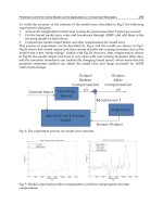
set of available input is reduced to one value, as it is shown in Fig. 3.


Fig. 3. LMPC strategy with fixed increment of the input during the control horizon and
constant value for the remaining time
Both search methods perform accurate path-tracking. Optimal input search has better time
performance and subinterval gradient descent method does not usually give the optimal
solution. Due to these facts obtained from simulations, complete input search is selected for
the on-robot experiences presented in the next section.

Using Model Predictive Control for Local Navigation of Mobile Robots

297
The evaluation of the LMPC performance is made by using different parametric values in the
proposed cost function (3). In this way, when only the desired coordinates are considered,
(P=1, Q=0, R=0, S=0), the trajectory-tracking is done with the inputs that can minimize the cost
function by shifting the robot position to the left. The reason can be found in Table 2, where
the right motor has more gain than the left one for high speeds. This problem can be solved,
(P=1, Q=1, R=0, S=0) or (P=1, Q=0, R=1, S=0) by considering either the straight-line trajectory
from the point where the last perception was done to the final desired point belonging to the
local field of perception or the predicted orientations. Simulated results by testing both
strategies provide similar satisfactory results. Thus, the straight line path or orientation should
be considered in the LMPC cost function. Fig. 4 shows a simulated result of LMPC for WMR
by using the orientation error, the trajectory distance and the final desired point for the cost
function optimization (P=1, Q=1, R=1, S=0). Obtained results show the need of R parameter
when meaningful orientation errors are produced.
The prediction horizon magnitude is also analyzed. The possible coordinates available for
prediction when the horizon is larger (n=10, m=5), depict a less dense possibility of coordinates
when compared with shorter horizons of prediction. Short prediction horizon strategy is more
time effective and performs path-tracking with better accuracy. For these reasons, a short
horizon strategy (n=5, m=3) is proposed for implementing experimental results.


Fig. 4. Trajectory tracking simulated result by using the orientation error, trajectory distance
and the final desired point for the optimization.
The sampling time for each LMPC step was set to 100ms. Simulation time performance of
complete input search and gradient descent methods is computed. For short prediction
horizon (n=5, m=3), the simulation processing time is less than 3ms for the complete input
search strategy and less than 1ms for the gradient descent method when algorithms are
running in a standard 2.7 GHz PC. Real on-robot algorithm time performance is also

compared for different prediction horizons by using the embedded 700 Mhz PC and
additional hardware system. Table 3 shows the LMPC processing time for different horizons
of prediction when complete optimal values search or the gradient descent method are used.
Surprisingly, when the horizon is increased the computing time is decreased. It is due to the
fact that the control horizon is also incremented, and consequently less range of signal
increments are possible because the signal increment is kept fixed within the control
horizon. Thus, the maximum input value possibilities decrease with larger horizons. Hence
for n=5 there are 1764 possibilities (42x42), and for n=10 there are 625 (25x25).

Advanced Model Predictive Control

298
Horizon of prediction
(n)
Complete
search method
Gradient
descent method
n=5 45ms 16ms
n=8 34ms 10ms
n=10 25ms 7ms
Table 3. LMPC processing times
3. Tuning the control law parameters by using path-tracking experimental
results
In this section, path-tracking problem and the cost function parameter weights are analyzed,
within a constrained field of perception provided by the on-robot sensor system. The main
objective is to obtain further control law analysis by experimenting different kind of
trajectories. The importance of the cost function parameter weights is analyzed by
developing the factorial design of experiments for a representative set of local trajectories.
Statistical results are compared and control law performance is analyzed as a function of the

path to be followed. Experimental LMPC results are conducted by considering a constrained
horizon of perception provided by a monocular camera where artificial potential fields are
used in order to obtain the desired coordinates within the field of view of the robot.
3.1 The local field of perception
In order to test the LMPC by using constrained local perception, the field of view obtained
by a monocular camera has been used. Ground available scene coordinates appear as an
image, in which the camera setup and pose knowledge are used, and projective perspective
is assumed to make each pixel coordinate correspond to a 3D scene coordinate (Horn, 1998).
Fig. 5 shows a local map provided by the camera, which corresponds to a field of view with
a horizontal angle of 48º, a vertical angle of 37º, H set to 109cm and a tilt angle of 32º.


Fig. 5. Available local map coordinates (in green), the necessary coordinates free of obstacles
and the necessary wide-path (in red).

Using Model Predictive Control for Local Navigation of Mobile Robots

299
It is pointed out that the available floor coordinates are reduced due to the WP (wide-path)
of the robot (Schilling, 1990). It should also be noted that for each column position
corresponding to scene coordinates Y
j
, there are R row coordinates X
i
. Once perception is
introduced, the problem is formulated as finding the optimal cell that brings the WMR close
to the desired coordinates (X
d
, Y
d

) by searching for the closest local desired coordinates (X
ld
,
Y
ld
) within the available local coordinates (X
i
, Y
j
). In this sense, perception is considered to
be a local receding horizon on which the trajectory is planned. The local desired cell is
obtained by minimizing a cost function J that should act as a potential field corridor. Thus,
the cost function is minimized by attracting the robot to the desired objective through the
free available local cell coordinates. It is noted that from local perception analysis and
attraction potential fields a local on field path can be obtained. The subsequent subsections
infer control law parameter analysis by considering a set of path possibilities obtained
within the perception field mentioned in this section.
3.2 The path-tracking experimental approach by using LMPC methods
The path tracking performance is improved by the adequate choice of a cost function that is
derived from (3) and consists of a quadratic expression containing some of the following
four parameters to be minimized:
•
The squared Euclidean approaching point distance (APD) between the local desired
coordinates, provided by the on-robot perception system, and the actual robot position.
It corresponds with the parameter “P” of the LMPC cost function given by (3).
•
The squared trajectory deviation distance (TDD) between the actual robot coordinate and
a straight line that goes from the robot coordinates, when the local frame perception
was acquired, and the local desired coordinates belonging to the referred frame of
perception. It corresponds with the parameter “Q” of the cost function shown by (3).

•
The third parameter consists of the squared orientation deviation (OD); it is expressed by
the difference between the robot desired and real orientations. It corresponds with the
parameter “R” of the LMPC cost function depicted by (3).
•
The last parameter refers to changes allowed to the input signal. It corresponds with the
parameter “S” of the LMPC cost function given by (3).
One consideration that should be taken into account is the different distance magnitudes. In
general, the approaching distance could be more than one meter. However, the magnitude
of the deviation distance is normally in the order of cm, which becomes effective only when
the robot is approaching the final desired point. Hence, when reducing the deviation
distance further to less than 1cm is attempted, an increase, in the weight value for the
deviation distance in the cost function, is proposed.
The subsequent subsections use statistical knowledge for inferring APD (P) and TDD (Q) or
APD (P) and OD (R) factor performances as a function of the kind of paths to be tracked.
Other cost function parameters are assumed to be equal to zero.
3.3 Experimental tuning of APD and TDD factors
This subsection presents the results achieved by using factorial design in order to study the
LMPC cost function tuning when APD and TDD factors are used. Path-tracking
performance is analyzed by the mean of the different factor weights. The experiments are
developed by considering five different kinds of trajectories within the reduced field of view
as shown in Fig. 5. Therefore, straight, wide left turning, less left turning, wide right turning

Advanced Model Predictive Control

300
and less right turning trajectories are tested. Experiments are conducted by using factorial
design with two levels of quantitative factors (Box et al, 2005). Referred to the cost function,
let us assume that high value (H) is equal to “1” and low value (L) is equal to “0.5”. For each
combination of factors three different runs are experimented. The averaged value of the

three runs allows statistical analysis for each factor combination. From these standard
deviations, the importance of the factor effects can be determined by using a rough rule that
considers the effects when the value differences are similar or greater than 2 or 3 times their
standard deviations. In this context, the main effects and lateral effects, related to APD and
TDD, are analyzed. Fig. 6 shows the four factor combinations (APD, TDD) obtained by both
factors with two level values.


Fig. 6. The different factor combinations and the influence directions, in which the
performances should be analyzed.
The combinations used for detecting lateral and main effect combinations are highlighted by
blue arrows. Thus, the main effect of APD factor, ME
APD
, can be computed by the following
expression:

32 10
22
APD
YY YY
ME
++
=−
(6)
Path-tracking statistical performances to be analyzed in this research are represented by Y.
The subscripts depict the different factor combinations. The main effect for TDD factor,
ME
TDD
, is computed by:

31 20
22
TDD
YYYY
ME
++
=−
(7)
The lateral effects are computed by using the following expression:

_30APD TDD
LE Y Y=− (8)
The detailed measured statistics with parameters such as time (T), trajectory error (TE), and
averaged speeds (AS) are presented in (Pacheco & Luo, 2011). The results were tested for
straight trajectories, wide and less left turnings, and wide and less right turnings. The main
and lateral effects are represented in Table 4.

Using Model Predictive Control for Local Navigation of Mobile Robots

301
The performance is analyzed for the different trajectories:
•
The factorial analysis for straight line trajectories, (σ
T
= 0.16s, σ
TE
= 0.13cm, σ
AS
=
2.15cm/s), depicts a main time APD effect of -0.45s, and an important lateral effect of -

0.6s and -0.32cm. Speed lateral effect of only 1.9cm/s is not considered as meaningful.
Considering lateral effects that improve time and accuracy, high values (APD, TDD) are
proposed for both factors.
•
The analysis for wide left turning trajectories, (σ
T
= 0.26s, σ
TE
= 0.09cm, σ
AS
= 0.54cm/s)
show negative APD main effect of 0.53s, and 0.15cm. However, the TDD factor tends to
decrease the time and trajectory deviation. The 0.3cm/s speed TDD main factor is
irrelevant. In this case, low value for APD factor and high value for the TDD factor is
proposed.
•
The factor analysis for less left turning, (σ
T
= 0.29s, σ
TE
= 0.36cm, σ
AS
= 0.84cm/s),
depicts a considerable lateral effect of -0.46s and -0.31cm. Speed -0.2cm/s lateral effect is
not important. In this sense high values are proposed for APD and TDD factors.
•
The analysis for wide right turning, (σ
T
= 0.18s, σ
TE

= 0.15cm, σ
AS
= 1.04cm/s) does not
provide relevant clues, but small time improvement seems to appear when TDD factor
is set to a low value. Low values are proposed for APD and TDD factors.
•
Finally, the factorial analysis for less right turning trajectories, (σ
T
= 0.12s, σ
TE
= 0.18cm,
σ
AS
= 1.94cm/s), depicts APD and lateral effects that increase the trajectory time with
0.32s and 0.44s. Main or lateral effects related to the speed have not been detected. Low
values are proposed for APD and TDD factors.

Straight line trajectory
Parameter
Performance
Main Effect
TDD factor
Main Effect
APD factor
Lateral Effect
TDD & APD factors
Time -0.05s -0.45s -0.6s
Trajectory accuracy -0.18cm -0.14cm -0.32cm
Averaged speed 1.25cm/s 0.6cm/s 1.9cm/s
Wide left turn trajectory

Time -0.34s 0.53s 0.16s
Trajectory accuracy -0.17cm 0.15cm -0.01cm
Averaged speed 0.3cm/s 0.4cm/s 0.7cm/s
Slight left turn trajectory
Time -0.24s 0.02s -0.46s
Trajectory accuracy -0.14cm -0.17cm -0.31cm
Averaged speed 0.8cm/s -1cm/s -0.2cm/s
Wide right turn trajectory
Time 0.27s -0.10s 0.17s
Trajectory accuracy -0.22cm 0.1cm -0.12cm
Averaged speed 0.7cm/s 0.2cm/s 0.9cm/s
Slight right turn trajectory
Time 0.12s 0.32s 0.44s
Trajectory accuracy -0.18cm -0.06cm -0.25cm
Averaged speed -1.3cm/s 2.8cm/s 1.5cm/s
Table 4. Main and lateral effects

Advanced Model Predictive Control

302
3.4 Experimental performance by using fixed or flexible APD & TDD factors
Once factorial analysis is carried out, this subsection compares path-tracking performance
by using different control strategies. The experiments developed consist in analyzing the
performance when a fixed factor cost function or a flexible factor cost function is used. The
trajectories to be analyzed are formed by straight lines, less right or left turnings, and wide
right or left turnings. The fixed factor cost function maintains the high values for APD and
TDD factors, while the flexible factor cost function is tested as function of the path to be
tracked.
Different experiments are done; see (Pacheco & Luo, 2011). As instance one experiment
consists in tracking a trajectory that is composed of four points ((0, 0), (-25, 40), (-25, 120), (0,

160)) given as (x, y) coordinates in cm. It consists of wide left turning, straight line and wide
right turning trajectories. The results obtained by using fixed and flexible factor cost
function are depicted in Table 5. Three runs are obtained for each control strategy and
consequently path-tracking performance analysis can be done.
Results show that flexible factor strategy improves an 8% the total time performance of the
fixed factor strategy. The turning trajectories are done near 50% of the path performed.
Remaining path consists of a straight line trajectory that is performed with same cost


Fig. 7. (a) Trajectory-tracking experimental results by using flexible or fixed cost function. (b)
WMR orientation experimental results by using flexible or fixed cost function. (c) Left wheel
speed results by using flexible or fixed cost function. (d) Right wheel speed results by using
flexible or fixed cost function.

Using Model Predictive Control for Local Navigation of Mobile Robots

303
function values for fixed and flexible control laws. It is during the turning actions, where the
two control laws have differences, when time improvement is nearly 16%. Fig. 7 shows an
example of some results achieved. Path-tracking coordinates, angular position, and speed
for the fixed and flexible cost function strategies are shown.
It can be seen that flexible cost function, when wide left turning is performed approximately
during the first three seconds, produces less maximum speed values when compared with
fixed one. However, a major number of local maximum and minimum are obtained. It
results in less trajectory deviation when straight line trajectory is commanded. In general
flexible cost function produces less trajectory error with less orientation changes and
improves time performance.


Trajectory points: (0,0), (-25,40), (-25,120), (0,160) ((x,y) in cm)

Time
(s)
Trajectory error
(cm)
Averaged Speed
(cm/s)
Experiment
Fixed
Law
Flexible
Law
Fixed
Law
Flexible
Law
Fixed
Law
Flexible
Law
Run 1 10,5 10,3 3,243 3,653 18,209 16,140
Run 2 10,9 9,8 3,194 2,838 16,770 16,632
Mean 10,70 10,05 3,219 3,245 17,489 16,386
Variance 0,0800 0,1250 0,0012 0,3322 1,0354 0,1210
Standart
deviation
0,2828 0,3536 0,0346 0,5764 1,0175 0,3479
Table 5. Results obtained by using fixed or flexible cost function
Developed experiences with our WMR platform show that flexible LMPC cost function
related with the path to be tracked can improve the control system performance.

3.5 Experimental tuning using APD and OD factors
In a similar way APD and OD factors can be used. This subsection compares path-tracking
performance by using different control strategies. The experiments developed consist in
analyzing the performance when a fixed factor cost function or a flexible factor cost function
is used. The trajectories to be analyzed are formed by straight lines, less right or left
turnings, and wide right or left turnings. The fixed factor cost function maintains the high
values for APD and OD factors, while the flexible factor cost function is tested as function of
the path to be tracked. The experiments developed show the measured performance
statistics, time, trajectory accuracy, and averaged speeds, for straight trajectories, wide and
less left turnings, and wide and less right turnings. The standard deviation obtained as well
as the main and lateral effects are represented in Table 6. The time, trajectory error and
averaged speed standard deviations are respectively denoted by σ
T
, σ
TE
, and σ
AS
. Table 6
represents the experimental statistic results obtained for the set of proposed trajectories. The
standard deviations computed for each kind of trajectory by testing the different factor
weights under different runs are also depicted.
The main and lateral effects were calculated by using (6), (7), (8), and the mean values
obtained for the different factor combinations. Therefore, in Table 6 are highlighted the

Advanced Model Predictive Control

304
significant results achieved using experimental factorial analysis. The inferred results
obtained can be tested using different trajectories.

Straight trajectory
Parameters
OD APD APD & OD
Time (s) σ
T
= 0.06s
0,02 -0,13 -0,10
Trajectory error (cm) σ
TE
= 0.69cm
-0,24 1,34 1,10
Speed (cm/s) σ
AS
= 0.88cm/s
0,87 0,70
1,57
Wide left turning
Parameters
OD APD APD & OD
Time (s) σ
T
= 0.06s
-0,10
0,20 0,10
Trajectory error (cm) σ
TE
= 0.18cm
0,36 0,38 0,02
Speed (cm/s) σ
AS

= 0.59cm/s
0,36 -0,87 -0,52
Less left turning
Parameters
OD APD APD & OD
Time (s) σ
T
= 0.09s
-0,12 0,07 -0,05
Trajectory error (cm) σ
TE
= 0.11cm
0,58 1,08 0,50
Speed (cm/s) σ
AS
= 0.92cm/s
0,60 -0,13 0,47
Wide right turning
Parameters
OD APD APD & OD
Time (s) σ
T
= 0.11s
0,10 0,35 0,45
Trajectory error (cm) σ
TE
= 0.08cm
0,44 0,45 0,01
Speed (cm/s) σ
AS

= 0.67cm/s
-0,58
-1,67 -2,25
Less right turning
Parameters
OD APD APD & OD
Time (s) σ
T
= 0.26s
-0,07 0,07 0,00
Trajectory error (cm) σ
TE
= 0.20cm
1,38 0,65 -0,73
Speed (cm/s) σ
AS
= 0.13cm/s
-0,33 -0,14 -0,48
Table 6. Main and lateral effects
The experiments developed consist in analyzing the time performance when a fixed factor
cost function or a flexible factor cost function is used. The trajectories to be analyzed are
formed by straight lines, less right or left turnings, and wide right or left turnings. The fixed
factor cost function maintains the high values for APD and OD factors, while the flexible
factor cost function is tested as function of the trajectory to be tracked. The experiments
presented consist in tracking a trajectory that is composed of three points ((0, 0), (-25, 40), (-
25, 120)) given as (x, y) coordinates in cm. The results obtained by using fixed and flexible
factor cost function are depicted in Table 7.

Using Model Predictive Control for Local Navigation of Mobile Robots

305
Trajectory (x,y) in cm: (0,0), (-25,40), (-25,120)
Features Time (s) Error (cm)
Aver. speed
(cm/s)
Experiment Fixed Flexible Fixed Flexible Fixed Flexible
Run 1 7,2 7,0 3,8 3,0 19,4 17,5
Run 2 7,4 6,6 2,2 3,5 16,5 20,1
Mean 7,3 6,8 3,0 3,2 18,0 18,8
Variance 0,02 0,1 1,3 0,1 4,2 3,4
Stand. dev. 0,14 0,3 1,1 0,3 2,0 1,9
Table 7. Experimental performances
Two runs are obtained for each strategy and consequently time performance analysis can be
done. The averaged standard deviation between the two cost function systems is of 0.22s,
and the difference of means are 0.5s. Thus, flexible factor strategy improves a 6.85% the time
performance of the fixed factor strategy. However, left turning is done only a 33% of the
trajectory. Thus, time improvement during the left turning is of near 20%. Fig. 8 shows an
example of some results achieved. Path-tracking coordinates, angular position, and speed
for the fixed and flexible cost function strategies are shown. Trajectory error and averaged
speed statistical results are not significant, due to the fact that the differences of means
between fixed and flexible laws are less than two times the standard deviations.
4. Conclusion
This research can be used on dynamic environments in the neighborhood of the robot. On-
line LMPC is a suitable solution for low level path-tracking. LMPC is more time expensive
when compared with traditional PID controllers. However, instead of PID speed control
approaches, LMPC is based on a horizon of available coordinates within short prediction
horizons that act as a reactive horizon. Therefore, path planning and convergence to
coordinates can be more easily implemented by using LMPC methods. In this way,
contractive constraints are used for guaranteeing the convergence towards the desired
coordinates. The use of different dynamic models avoids the need of kinematical constraints

that are inherent to other MPC techniques applied to WMR. In this context the control law is
based on the consideration of two factors that consist of going straight or turning. Therefore,
orientation deviation or trajectory deviation distance can be used as turning factors. The
methodology used for performing the experiments is shown. From on-robot depicted
experiences, the use of flexible cost functions with relationships to the path to be tracked can
be considered as an important result. Thus, control system performance can be improved by
considering different factor weights as a function of path to be followed.
The necessary horizon of perception is constrained to just few seconds of trajectory
planning. The short horizons allow real time implementations and accuracy trajectory
tracking. The experimental LMPC processing time was 45ms, (m=3, n=5), running in the
WMR embedded PC of 700MHz. The algorithms simplicity is another relevant result
obtained. The factorial design, with two levels of quantitative factors, is presented as an easy
way to infer experimental statistical data that allow testing feature performances as function


Advanced Model Predictive Control

306








Fig. 8. (a) Trajectory-tracking experimental results by using flexible or fixed cost function. (b)
WMR orientation experimental results by using flexible or fixed cost function. (c) Left wheel
speed results by using flexible or fixed cost function. (d) Right wheel speed results by using
flexible or fixed cost function.

of the different factor combinations. Further studies on LMPC should be done in order to
analyze its relative performance with respect to other control laws or to test the cost function
performance when other factors are used. The influence of the motor dead zones is also an
interesting aspect that should make further efforts to deal with it.
5. Acknowledgement
This work has been partially funded by the Commission of Science and Technology of Spain
(CICYT) through the coordinated projects DPI2007-66796-C03-02 and DPI 2008-06699-C02-
01.

Using Model Predictive Control for Local Navigation of Mobile Robots

307
6. References
Box, G. E. P., Hunter, J. S., Hunter W. G. (2005). Statistics for Experimenters, Ed. John Wiley
& Sons, ISBN 0-471-71813-0, New Jersey (USA).
Boyd, S. & Vandenberghe, L. (2004). Convex Optimization, Cambridge University Press,
ISBN-13: 9780521833783, New York (USA).
Fox, D.; Burgard, W. & Thrun, S. (1997). The dynamic window approach to collision
avoidance. IEEE Robotics & Automation Magazine, Vol. 4, No. 1, (Mar 1997) 23-33,
ISSN 1070-9932
Gupta, G.S.; Messom, C.H. & Demidenko, S. (2005). Real-time identification and predictive
control of fast mobile robots using global vision sensor. IEEE Trans. On Instr. and
Measurement, Vol. 54, No. 1, (February 2005) 200-214, ISSN 1557-9662
Horn, B. K. P. (1998). Robot Vision. MIT press, Ed. McGraw–Hill, ISBN 0-262-08159-8,
London (England)
Klancar, G & Skrjanc, I. (2007). Tracking-error model-based predictive control for mobile
robots in real time, Robotics and Autonomous Systems, Vol. 55, No. 6, (June 2007 ),
pp. 460-469, ISSN: 0921-8890.
Kühne, F.; Lages, W. F. & Gomes da Silva Jr., J. M., (2005). Model predictive control of a
mobile robot using input-output linearization, Proceedings of Mechatronics and

Robotics, ISBN 0-7803-9044-X, Niagara Falls Canada, July 2005
Ljung, L. (1991). Issues in System Identification. IEEE Control Systems Magazine, Vol. 11,
No.1, (January 1991) 25-29, ISSN 0272-1708
Maciejowski, J.M. (2002). Predictive Control with Constraints, Ed. Prentice Hall, ISBN 0-201-
39823-0, Essex (England)
Nesterov, I. E.; Nemirovskii, A. & Nesterov, Y. (1994). Interior_Point Polynomial Methods
in Convex Programming. Siam Studies in Applied Mathematics, Vol 13,
Publications, ISBN 0898713196
Norton, J. (1986). An Introduction to Identification. Academic Press, ISBN 0125217307,
London and New York, 1986
Ögren, P. & Leonard, N. E. (2005). A convergent dynamic window approach to obstacle
avoidance. IEEE Transaction on Robotics, Vol. 21, No. 2., (April 2005) 188-195,
ISSN: 1552-3098
Pacheco, L., Luo, N., Cufí, X. (2008). Predictive Control with Local Visual Data, In: Robotics,
Automation and Control, Percherková, P., Flídr, M., Duník, J., pp. 289-306,
Publisher I-TECH, ISBN 978-953-7619-18-4, Printed in Croatia.
Pacheco, L., Luo, N.; Ferrer, I. and Cufí, X. (2009). Interdisciplinary Knowledge Integration
Through an Applied Mobile Robotics Course, The International Journal
of Engineering Education, Vol. 25, No. 4, (July, 2009), pp. 830-840, ISSN:
0949-149X
Pacheco, L., Luo, N. (2011) Mobile robot local trajectory tracking with dynamic
model predictive control techniques, International Journal of Innovative
Computing, Information and Control, Vol.7, No.6, (June 2011), in press, ISSN 1349-
4198
Schilling, R.J. (1990). Fundamental of Robotics. Prentice-Hall (Ed.), New Jersey (USA) 1990,
ISBN 0-13-334376-6

Advanced Model Predictive Control

308

Wan, J. (2007) Computational reliable approaches of contractive MPC for discrete-time
systems, PhD Thesis, University of Girona.
15
Model Predictive Control and Optimization
for Papermaking Processes
Danlei Chu, Michael Forbes, Johan Backström,
Cristian Gheorghe and Stephen Chu
Honeywell,
Canada
1. Introduction
Papermaking is a large-scale two-dimensional process. It has to be monitored and controlled
continuously in order to ensure that the qualities of paper products stay within their
specifications. There are two types of control problems involved in papermaking processes:
machine directional (MD) control and cross directional (CD) control. Machine direction
refers to the direction in which paper sheet travels and cross direction refers to the direction
perpendicular to machine direction. The objectives of MD control and CD control are to
minimize the variation of the sheet quality measurements in machine direction and cross
direction, respectively. This chapter considers the design and applications of model
predictive control (MPC) for papermaking MD and CD processes.
MPC, also known as moving horizon control (MHC), originated in the late seventies and has
developed considerably in the past two decades (Bemporad and Morari 2004; Froisy 1994;
Garcia et al. 1998; Morari & Lee 1999; Rawlings 1999; Chu 2006). It can explicitly incorporate
the process’ physical constraints in the controller design and formulate the controller design
problem into an optimization problem. MPC has become the most widely accepted advanced
control scheme in industries. There are over 3000 commercial MPC implementations in
different areas, including petro-chemicals, food processing, automotives, aerospace, and pulp
and paper (Qin and Badgwell 2000; Qin and Badgwell 2003).
Honeywell introduced MPC for MD controls in 1994; this is likely the first time MPC
technology was applied to MD controls (Backström and Baker, 2008). Increasingly, paper
producers are adopting MPC as a standard approach for advanced MD controls.

MD control of paper machines requires regulation of a number of quality variables, such as
paper dry weight, moisture, ash content, caliper, etc. All of these variables may be coupled
to the process manipulated variables (MV’s), including thick stock flow, steam section
pressures, filler flow, machine speed, and disturbance variables (DV’s) such as slice lip
adjustments, thick stock consistency, broke recycle, and others. Paper machine MD control
is truly a multivariable control problem.
In addition to regulation of the quality variables during normal operation, a modern
advanced control system for a paper machine may be expected to provide dynamic
economic optimization on the machine to reduce energy costs and eliminate waste of raw
materials. For machines that produce more than one grade of paper, it is desired to have an
automatic grade change feature that will create and track controlled variable (CV) and MV

Advanced Model Predictive Control
310
trajectories to quickly and safely transfer production from one grade to the next. Basic MD-
MPC, economic optimization, and automatic grade change are discussed in this chapter.
MPC for CD control was introduced by Honeywell in 2001 (Backström et al. 2001). Today,
MPC has become the trend of advanced CD control applications. Some successful MPC
applications for CD control have been reported in (Backström et al. 2001, Backström et al.
2002; Chu 2010a; Gheorghe 2009).
In papermaking processes, it is desired to control the CD profile of quality variables such as
dry weight, moisture, thickness, etc. These properties are measured by scanning sensors that
traverse back and forth across the paper sheet, taking as many as 2000 or more samples per
sheet property across the machine. There may be several scanners installed at different
points along the paper machine and so there may be multiple CD profiles for each quality
variable.
The CD profiles are controlled using a number of CD actuator arrays. These arrays span the
paper machine width and may contain up to 300 individual actuators. Common CD
actuators arrays allow for local adjustment, across the machine, of: slice lip opening,
headbox dilution, rewet water sprays, and induction heating of the rolls. As with the CD

measurements, there may be multiple CD actuator arrays of each type available for control.
By changing the setpoints of the individual CD actuators within an array, one can adjust the
local profile of the CD measurements.
The CD process is a multiple-input-multiple-output (MIMO) system. It shows strong input
and output off-diagonal coupling properties. One CD actuator array can have impact on
multiple downstream CD measurement profiles. Conversely, one CD measurement profile can
be affected by multiple upstream CD actuator arrays. Therefore, the CD control problem
consists of attempting to minimize the variation of multiple CD measurement profiles by
simultaneously optimizing the setpoints of all individual CD actuators (Duncan 1989).
MPC is a natural choice for paper machine CD control because it can systematically handle
the coupling between multiple actuator and multiple measurement arrays, and also
incorporate actuator physical constraints into the controller design. However, different from
standard MPC problems, the most challenging part of the cross directional MPC (CD-MPC)
is the size of the problem. The CD-MPC problem can involve up to 600 MVs, 6000 CVs, and
3000 hard constraints. Also, the new setpoints of MVs are required as often as every 10 to 20
seconds. This chapter discusses the details of the design for an efficient large-scale CD-MPC
controller.
This chapter has 5 sections. Section 2 provides an overview of the papermaking process
highlighting both the MD and CD aspects. Section 3 focuses on modelling, control and
optimization for MD processes. Section 4 focuses on modelling, control and optimization for
CD processes. Both Sections 3 and 4 give industrial examples of MPC applications. Finally,
Section 5 draws conclusions and provides some perspective on the future of MD-MPC and
CD-MPC.
2. Overview of papermaking processes
A flat sheet of paper is a network consisting of cellulose fibres bound to one another. A
paper machine transforms a slurry of water and wood cellulose fibres into this type of
network. The whole papermaking process can be regarded as a water-removal system: the
consistency of fibre solutions, called stock by papermakers, increases from around 1% at the
beginning of a paper machine (the headbox) to around 95% at the end (the reel).

Model Predictive Control and Optimization for Papermaking Processes
311
2.1 Brief description of papermaking processes
In general a paper machine can be divided into four sections: forming section, press section,
drying section, and calendering section. In the forming section, the stock flow enters the
headbox to be distributed evenly across a continuously running fabric felt called the wire.
The newly formed sheet is carried by the wire along the Fourdrinier table, which has a set of
drainage elements that promote water removal by various gravity and suction mechanisms.
These elements include suction boxes, couch rolls, foils, etc. The solid consistency of the
paper web can reach 20% by the time the web leaves the forming section and enters the
press section. Figure 1 illustrates the configuration of a Fourdrinier-type paper machine.


Fig. 1. The configuration of a Fourdrinier-type paper machine
The press section may be considered as an extension of the water-removal process that was
started on the wire in the forming section. Typically, it consists of 1 – 3 rolling press nips.
When the paper web passes through these nips, the pressing roll squeezes water out and
consolidates the web formation at the same time. In the press section, both the surface
smoothness and the web strength are improved. As higher web strength is achieved in the
press section, better runability will be observed in the drying section. A paper machine is
typically operated at a very high speed. The fastest machine speed may be as high as 2,200
meters per minute.
The drying section includes multiple drying cylinders which are heated by high temperature
and high pressure steam. The heat is transferred from steam onto the paper surface through
these rotating steel cylinders. The heat flow increases the paper surface temperature to the
point where water starts evaporating and escaping from the paper web. The drying section is
the most energy consuming part of paper manufacturing. Before the paper enters the drying
section, the solid consistency is around 50%. After the drying section, the consistency can reach
95%, which corresponds to a finished product moisture specification.
The last section of the paper machine is called the calendering section. Calendering is a

terminology referring to pressing with a roll. The surface and the interior properties of the
paper web are modified when it passes through one or more calendering nips. Typically the
calendering nip consists of one or multiple soft/hard or hard/hard roll pairs. The hard roll
presses the paper web against the other roll, and deforms the paper web plastically. By this
means, the calender roll surface is replicated onto the paper web. Depending on the type of
paper being produced, the primary objective of calendering may be to produce a smooth
paper surface (for printing), or to improve the uniformity of CD properties, such as paper
caliper (thickness).

Advanced Model Predictive Control
312
More details of paper machine design and operation are given in (Smook 2002; Gavelin
1998).
2.2 Paper quality measurement
A paper machine can have one or more measurement scanners. The quality measurement
sensors are mounted on the scanner head which travels back and forth across the paper web
to provide online quality measurements. The most common paper machine quality
measurements include dry weight, moisture, and caliper. Dry weight indicates the solid
weight per unit area of a sheet of paper. For different types of products, the value of dry
weight can vary from 10 grams per square meter (gsm), in the case of paper tissue, to 400
gsm, in the case of heavy paper board. Moisture content is another critical quality property
of the finished paper product. It indicates the mass percentage of water contained in a sheet
of paper. Moisture content is a key factor determining the strength of the finished product.
Typical moisture targets range from 5% to 9%. Caliper is the measure of the thickness of a
sheet of paper. It is a key factor determining the gloss and printability of the finished
product. The caliper targets are in the range from 70μm to 300 μm depending on the
production grade. In general the online measurements for dry weight, moisture and caliper
are available and used for both the MD and CD feedback controller designs.
As the scanners travel across a moving sheet, the real data collected actually comes from a
zig-zag trajectory (See Figure 2). These data contain both CD and MD variation. A reliable

MD/CD separation scheme is the prerequisite for MD and CD control designs. Since the
MD/CD separation is a separate topic, the rest of this chapter assumes that the pure
MD/CD measurements have been obtained prior to the MD/CD controller development.
The scanner measurements are denoted by x(i, t), i=1,⋯,n indexes the n measurements
taken across the sheet each scan (CD measurement index), and t is the time stamp of each
scan (MD measurement index). x(t) is the MD measurement given by
x(t)=
1
n
∑
x(i, t)
n
i=1
. (1)


Fig. 2. The zig-zag scanner trajectories

Model Predictive Control and Optimization for Papermaking Processes
313
2.3 Brief description of MD control
The objective of MD control is to minimize the variation of the sheet quality measurements
in machine direction.
A number of actuators are available for control of the MD variables. Stock flow to the headbox
is regulated by the stock flow valve or variable speed pump. As stock flow increases, the
amount of fibre flowing into the forming section increases and dry weight and caliper increase.
At the same time, there is also more water coming through the machine and moisture will
increase. So, changes in the stock flow affect dry weight, moisture and caliper. The steam
pressure in the cylinders of the drying section may be adjusted. As the steam pressure in the
cylinders increases, so does the temperature in the cylinders, and more heat is transferred to

the paper. In this way, steam pressure affects moisture. Typically, the dryer cylinders are
divided into groups, and the steam pressure for each of these dryer sections may be adjusted
independently. Machine speed affects dry weight and caliper, as increasing the machine speed
stretches the paper web thinner, giving it less mass per unit area. Machine speed also affects
moisture as both the drying properties of the paper and the residence time in the dryer change.
Clearly, paper machine MD control is a multivariable control problem.
2.4 Brief description of CD control
The objective of CD control is to achieve uniform paper qualities in the cross direction, i.e.,
to minimize the variation of CD profiles. The CD variation, can be formulated as two times
of the standard deviation of the CD profile,
2σ
CD
(t)=2* 
1
n-1
∑
(x(i, t)-x(t))
2
n
i=1

1
2
(2)
Often the term ‘CD spread’ is used interchangeably with 2σ
CD
.
CD actuators are used to regulate CD profiles and improve the uniformity of paper quality
properties in the cross direction i.e., reduce the value of 2σ
CD

.
The most common dry weight CD actuators are both located at the headbox. The headbox
slice opening is a full-width orifice or nozzle that can be adjusted at points across the width
of the paper machine. This allows for differences in the local stock flow onto the wire across
the machine. The consistency profiler changes the consistency of local stock flow by injecting
dilution water and altering the local concentration of pulp fibre across the headbox.
Headbox slice and consistency profiler are primarily designed for dry weight control, but
they have the effects on both moisture and caliper profiles. Figure 1 indicates the location of
headbox dry weight actuators.
The most common moisture actuators are the steam box and water spray. The steam box
applies high temperature steam to the surface of the moving paper web. As the latent heat in
the steam is released and heats up the paper web, it lowers the web viscosity and eases
dewatering in the press section. The water spray regulates the moisture profiles according to
a different mechanism. It deploys a fine water spray to the paper surface through a set of
nozzles across the machine width to re-moisturize the paper web. Similar to the dry weight
actuators, moisture actuators are designed for moisture profile regulation but they may have
effects on the caliper profile. The steam box is typically installed in the press section and the
water spray is located in the drying section. Figure 1 indicates the physical locations of
moisture actuators.
The most common caliper actuators are hot air showers and induction heaters. Both types of
actuators provide surface heating for calendering rolls. The hot shower uses the high