Advanced Model Predictive Control Part 12 potx

Model Predictive Control and Optimization for Papermaking Processes
319
that the highest costing MV’s are driven to their minimum operating points, and the lowest
costing MV’s are driven to their maximum operating points. The TAD1 dry end differential
pressure is left as the MV that is within limits and actively controlling the paper moistures.
Figure 10 shows that throughout this trial, the MV’s are optimized without causing any
disturbance to the CV’s.




Fig. 5. The MPC model matrix for the tissue machine control and optimization example




Fig. 6. Natural gas costs and electricity costs during the trial
Stock
Flow
TAD1
Supply
Temp
TAD1 DE
DP
TAD1
Gap Pres
TAD2 Exh
Temp
TAD2 DE
DP

TAD2
Gap Pres
Yankee
Hood
Temp
Yankee
Supply
Fan
S
p
eed
Machine
Speed
Stock
Flow
TAD1
Gap
Pressure
Tickler
Refiner
Dry Weight
Reel
Moisture
TAD
Moisture
TAD1
Exhaust
Pressure

Advanced Model Predictive Control

320









Fig. 7. Total costs during the trial









Table 2. The MV cost rankings.
MV eng unit Low Limit High Limit
Linear Obj
Coef
(Cost/eng unit)
Process
Gain
(%Moi/eng unit)
Cost
(Cost / %

Moi) Rank
Optimization
Behavior
TAD1 Supply Temp deg F 300.0 450.0 0.68 -0.12 5.48 4
450 (max)
TAD1 DE DP inch H2O 1.0 3.9 47.30 -5.12 9.24 3 controlling Moi
TAD1 Gap Prs inch H2O 0.4 1.5 -0.03 1.95 0.02 6
0.4 (max)
TAD2 Exh Temp deg F 175.0 250.0 5.86 -0.45 13.02 1
175 (min)
TAD2 DE DP inch H2O 1.0 3.5 40.26 -3.14 12.82 2
1 (min)
TAD2 Gap Prs inch H2O 0.2 1.5 -16.40 4.25 3.86 5
0.2 (max)

Model Predictive Control and Optimization for Papermaking Processes
321

Fig. 8. Manipulated variables during the trial


Fig. 9. Manipulated variables during the trial

Advanced Model Predictive Control
322

Fig. 10. Controlled variables during the trial
3.4 Grade change strategies
Grade change is a terminology in MD control. It refers to the process of transitioning a paper
machine from producing one grade of paper product to another. One can achieve a grade

change by gradually ramping up a set of MVs to drive the setpoints of CVs from one
operating point to another. During a grade change, the paper product is often off-
specification and not sellable. It is important to develop an automatic control scheme to
coordinate the MV trajectories and minimize the grade change transition times and the off-
spec product. An offline model predictive controller can be designed to produce CV and
MV trajectories to meet these grade change criteria. MPC is well-suited to this problem
because it explicitly considers MV and CV trajectories over a finite horizon. By coordinating
the offline grade change controller (linear or nonlinear) and an online MD-MPC, one can
derive a fast grade change that minimizes off-spec production. This section discusses the
design of MPC controllers for linear and nonlinear grade changes.
Figure 11 gives a block diagram of the grade change controller incorporated into an MD
control system. The grade change controller calculates the MV and CV trajectories to meet
the grade change criteria. This occurs as a separate MPC calculation performed offline so
that grade change specific process models can be used, and so that the MPC weightings can
be adjusted until the MV and CV trajectories meet the design criteria. The MV trajectories
are sent to the regulatory loop as a series of MV setpoint changes. The CV trajectories are
sent as setpoint changes to the MD controller. If the grade change is performed with the MD
controller in closed-loop, additional corrections to the MV setpoints are made to eliminate
any deviation of the CV from its target trajectory.
Controlled Variables
11.6
11.7
11.8
11.9
12
12.1
12.2
12.3
12.4
12.5

12.6
12.7
8:34:07
8:40:34
8:47:01
8:53:28
8:59:55
9:06:22
9:12:49
9:19:16
9:25:43
9:32:10
9:38:37
9:45:04
9:51:31
9:57:58
10:04:25
10:10:52
10:17:19
10:23:46
10:30:13
10:36:40
10:43:07
10:49:34
10:56:01
11:02:28
11:08:55
11:15:22
11:21:49
11:28:16

11:34:43
11:41:10
11:47:37
11:54:04
12:00:31
12:06:58
12:13:25
12:19:52
Time
DW (lb/ream)
0
5
10
15
20
25
Moisture (%)
ReelDwt PV ReelMoi PV ExpressMoi PV

Model Predictive Control and Optimization for Papermaking Processes
323

Fig. 11. Block diagram of MD-MPC control enhanced with grade change capability
The MV and CV trajectories are generated in a two step procedure. First there is a target
calculation step that generates the MV setpoints required to bring the CV’s to their target
values for the new grade. Once the MV setpoints are generated, then there is a trajectory
generation step where the MV and CV trajectories are designed to meet the specifications of
the grade change.
The MV targets are generated from solving a set of nonlinear equations:

()
()
()
()
11
dw dw 1 2 3 1 2 3
22
dw dw 1 2 3 1 2 3
11
moi moi 1 2 3 1 2 3
22
moi moi 1 2 3 1 2 3
y f u ,u ,u , ,C ,C ,C , 0,
y f u ,u ,u , ,C ,C ,C , 0,
y f u ,u ,u , ,C ,C ,C , 0,
y f u ,u ,u , ,C ,C ,C , 0,
−……=
−……=
−……=
−……=


(11)
Here y
dw
/y
moi
represents the CV target for the new grade. The functions f
(
∙

)
are the
models of dry weight and moisture. The process MV’s are denoted u
i
and model constants
are denoted C
i
. The superscripts indicate the same paper properties measured by different
scanners. Since the number of MV’s and the number of CV’s is not necessarily equal, these
equations may have one, multiple or no solutions. To allow for all of these cases, the
problem is recast as:

min


F
(
u

,u

,…
)
, (12)
Subject to:
G
(
u

,u


,…
)
≤0,
H
(
u

,u

,…
)
=0,

Grade Change
Controller
Process
Scanner
R
1
R
2
MD - MPC
Operator
Operator
u
1,OP

u
2,OP

y
2

y
1
u
C1,SP
u
1,SP
Δu
1,GC
u
2,SP
u
C2,SP
y
1,SP

y
1,SP
y
2,SP

y
2,SP

User Input

Advanced Model Predictive Control
324

Where F
(
∙
)
is a quadratic objective function formulated to find the minimum travel solution.
H
(
∙
)
represents the equality constraints given above, and G
(
∙
)
represents the physical
limitations of the CVs and MVs (high, low, and rate of change limits).
Once the MV targets have been generated, the MV and CV trajectories are then designed.
Figure 12 gives a schematic representation of the trajectory generation algorithm. The
process models are linearized (if necessary) and then scaled and normalized for
application in an MPC controller. Process constraints such as the MV and CV targets, and
the MV high and low limits are also given to the MPC controller. Internal controller
tuning parameters are then used to adjust the MV and CV trajectories to meet the grade
change requirements.


Fig. 12. Diagram of MPC-based grade change trajectory generation.
3.4.1 Linear grade change
In a linear grade change, the MD process models that are used in the MD-MPC controller
are also used as the models for determining the MD targets, and for designing the MD grade
change trajectories.
3.4.2 Nonlinear grade change

In a nonlinear grade change, a first principles model may be used for the target and
trajectory generation. For example, a simple dry weight model is:

m

=K



, (13)

MPC Module
Linearization Nonlinear Model
MPC Controller Process Model
Scaling &
Normalization
Grade Change Constraints
• MV physical limits
• MV and CV targets
• Customized Weights
CV Target
CV Trajectories
MV Trajectories

Model Predictive Control and Optimization for Papermaking Processes
325
Where m

is the paper dry weight, q


is the thick stock flow, and v is machine speed. K
is the expression of a number of process constants and values including fibre retention,
consistency, and fibre density. (Chu et al. 2008) gives a more detailed treatment of this dry
weight model.
(Persson 1998, Slätteke 2006, and Wilhelmsson 1995) are examples of first principles
moisture models that may be used.
3.4.3 Mill implementation results
In this section, some results of MPC-based grade changes for a fine paper machine are given.
The grade change is from a paper with a dry weight of 53 lb/3000ft
2
(86 g/m
2
) to a paper
with a dry weight of 44 lb/3000ft
2
(72 g/m
2
). Both paper grades have the same reel moisture
setpoint of 4.8%. For the grade change, stock flow, 6
th
section steam pressure, and machine
speed are manipulated.
Figures 13 and 14 show a grade change performed on the paper machine using linear
process models, and keeping the regular MPC in closed-loop during the grade change. The
grade change was completed in 10 minutes, which is a significant improvement over the 22
minutes required by the grade change package of the plant’s previous control system. In
Figure 13, the CV trajectories are shown. Here it can be seen that although there is initially a
small gap between the actual dry weight and the planned trajectory, the regular MPC takes
action with the thick stock valve (as shown in Figure 14) to quickly bring dry weight back on
target. The deviation in the reel moisture is more obvious. This might be expected as the

moisture dynamics of the paper machine display more nonlinear behaviour for this range of
operations. The steam trajectory in Figure 14 is ramping up at its maximum rate and yet the
paper still becomes too wet during the initial part of the grade change. This indicates that
the grade change package is aggressively pushing the system to achieve short grade change
times.


Fig. 13. CV trajectories under closed-loop GC with linear models

Advanced Model Predictive Control
326

Fig. 14. MV trajectories under closed-loop GC with linear models
Figures 15 and 16 show a grade change performed on a high fidelity simulation of the fine
paper machine. This grade change uses a nonlinear process model, and the regular MPC is
kept in closed-loop during the grade change. Here it can be seen that the duration of the
grade change is reduced to 8 minutes. Part of the improvement comes from using stock flow
setpoint instead of stock valve position, allowing improved dry weight control. Another
improvement is that the planned trajectories allow for some deviation in the reel moisture
that cannot be eliminated. Both dry weight and reel moisture follow their trajectories more
closely. At the end of the grade change, the nonlinear grade change package is able to
anticipate the need to reduce steam preventing the sheet from becoming dry.


Fig. 15. CV trajectories under closed-loop GC with nonlinear models

Model Predictive Control and Optimization for Papermaking Processes
327

Fig. 16. MV trajectories under closed-loop GC with nonlinear models

4. Modelling, control and optimization of papermaking CD processes
To produce quality paper it is not enough that the average value of paper weight, moisture,
caliper, etc across the width of the sheet remains on target. Paper properties must be
uniform across the sheet. This is the purpose of CD control.
4.1 Modelling of papermaking CD processes
The papermaking CD process is a large scaled two-dimensional process. It involves multiple
actuator arrays and multiple quality measurement arrays. The process shows very strong
input-output off-diagonal coupling properties. An accurate CD model is the prerequisite for
an effective CD-MPC controller. We begin by discussing a model structure for the CD
process and the details of the model identification.
4.1.1 A two-dimensional linear system
The CD process can be modelled as a linear multiple actuator arrays and multiple
measurement arrays system,
Y(s)=G(s)U(s)+D(s), (14)
and
Y(s)=
y

(s)
⋮
y


(s)
,G(s)=
G

(s) … G



(s)
⋮⋱⋮
G



(s) … G




(s)
, U(s)=
u

(s)
⋮
u


(s)
, (15)

Advanced Model Predictive Control
328
where Y(s)∈ℂ
(

⋅)
is the Laplace transformation of the augmented CD measurement

array. The element
y

(s)∈ℂ

(i=1,…,N

) is the Laplace transformation of the i
th

individual CD measurement profile, such as dry weight, moisture, or caliper.
N

is the total
number of the quality measurements, and m is the number of elements of individual
measurement arrays.
U(s)∈ℂ
(
∑





)
is the Laplace transformation of the augmented
actuator setpoint array. The element
u

(s)∈ℂ



(j=1…N

) is the Laplace transformation of
the j
th
individual CD actuator setpoint profile, such as the headbox slice, water spray, steam
box, or induction heater.
N

is the total number of actuator beams available as MV’s, and n


is the number of individual zones of the jth actuator beam. In general a CD system has the
same number of elements for all CD measurement profiles, but different numbers of
actuator beam setpoints. D(s)
∈ℂ
(

⋅)
is the Laplace transformation of the augmented
process disturbance array. It represents process output disturbances.
G

(s)∈ℂ
×

(i=1…N


andj=1…N

) in (15) is the transfer matrix of the sub-system
from the j
th
actuator beam u

to the i
th
CD quality measurement y

. The model of this sub-
system can be represented by a spatial static matrix
P

∈ℝ
×

with a temporal dynamic
transfer function
h

(s). In practice, h

(s) is simplified as a first-order plus dead time
system. Therefore,
G

(s) is given by

G

(s)=P

h

(s)=P





e



(16)
where
T

is the time constant and T

is the time delay. The static spatial matrix P

is a matrix
with
n

columns, i.e., P


=
[
p

p

⋯p


]
and its kth column p

represents the spatial
response of the k
th
individual actuator zone of the j
th
actuator beam. As proposed in
(Gorinevsky & Gheorghe 2003),
p

can be formulated by,

22
kk
22
α((x x ) βω) α((x x ) βω)
k
ωω
kk

g
ππ
p{e cos(((xx)βω)) ecos(((xx)βω))}
2 ωω
−− −+
−−
=−−+−+ (17)
where x is the coordinate of CD measurements (CD bins), g is the process gain,
ω is the
response width,
α is the attenuation and β is divergence. x

is the CD alignment that
indicates the spatial relationship between the centre of the k
th
individual CD actuator and
the center of the corresponding measurement responses. A fuzzy function may be used to
model the CD alignment. Refer to (Gorinevsky & Gheorghe 2003) for the technical details.
Figure 17 illustrates the structure of the spatial response matrix
P

. The colour map on the
left shows the band-diagonal property of
P

; and the plot in the right shows the spatial
response of the individual spatial actuator
p

. It can be seen that each individual actuator

affects not only its own spatial zone area, but also adjacent zone areas.
4.1.2 Model identification
Model identification of the papermaking CD process is the procedure to determine the
values of the parameters in (16, 17), i.e., the dynamic model parameters
θ

={T

,T

}, the
spatial model parameters
θ

={g,ω,α,β}, and the alignment x

. An iterative identification
algorithm has been proposed in (Gorinevsky & Gheorghe 2003). As with MD model
identification, this algorithm is an open-loop model identification approach. Identification
experiment data are first collected by performing open-loop bump tests.

Model Predictive Control and Optimization for Papermaking Processes
329

Fig. 17. The illustration to spatial response matrix P

.
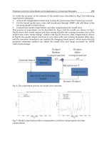
Figure 18 illustrates the logic flow of this algorithm. This nontrivial system identification
approach first estimates the overall dynamic response and spatial response, and
subsequently identifies the dynamic model parameter θ


and the spatial model
parameterθ

. h

in Figure 18 is the estimated finite impulse response (FIR) of the dynamic
model h(s) in (16). p in Figure 18 is the estimated steady state measurement profile, i.e.,
overall spatial response. For easier notation, we omit the indexes i and j here. The key
concept of the algorithm is to optimize the model parameters iteratively. Refer to
(Gorinevsky & Gheorghe 2003) for technical details of this algorithm, and (Gorinevsky &
Heaven, 2001) for the theoretical proof of the algorithm convergence.


Fig. 18. The schematic of the iterative CD system identification algorithm
The algorithm described above has been implemented in a software package, named
IntelliMap
TM
, which has been widely used in pulp and paper industries. The tool executes
the open-loop bump tests automatically and, at the end of the experiments, provides a
continuous-time transfer matrix model (defined in (14)). For convenience, the MPC
controller design discussed in the next section will use the state space model representation.
Conversion of the continuous-time transfer matrix model into the discrete-time state space
model is trivial (Chen 1999) and is omitted here.

Advanced Model Predictive Control
330
4.2 CD-MPC design
In this section, a state space realization of (14) is used for the MPC controller development,

X(k+1) =AX(k)+BΔU(k)
Y(k) =CX(k)+D(k)
. (18)
X(k)∈ℝ
(⋅

⋅)
, Y(k)∈ℝ
(

⋅)
, ΔU(k)∈ℝ
(
∑





)
,andD(k)∈ℝ
(

⋅)
are the augmented
state, output, actuator move, and output disturbance arrays of the papermaking CD process
with multiple CD actuator beams and multiple quality measurement arrays. {A, B, C} are the
model matrices with compatible dimensions. Assume (A, B) is controllable and (A, C) is
observable. In this section, the objective function of CD-MPC is developed first. Then the CD
actuator constraints are incorporated in the objective function. Finally a fast QP solver is

presented for solving the large scale constrained CD-MPC optimization problem. How to
tune a CD-MPC controller is also covered in this section
4.2.1 Objective function of CD-MPC
The first step of MPC development is performing the system output prediction over a
certain length of prediction horizon. From the state space model defined in (18), we can
predict the future states,

(k) =

X(k)+

Δ(k)
, (19)
where
(k)∈ℝ
(⋅

⋅⋅

)
is the state prediction, Δ(k)∈ℝ
(
⋅
∑





)

is the augmented
actuator moves.


and 

are the state and input prediction matrices with the compatible
dimensions.
H

and H

are the output and input prediction horizons, respectively.
The explicit expressions of the parameters in (19) are

ppu
p
2
AB
H1 HH
H
p
u
A
B0
X(k 1|k)
AB 0
X(k 2|k)
A
(k) , , ,

X(k H |k)
AB A B
A
ΔU(k|k)
ΔU(k 1|k)
and Δ (k)
ΔU(k H 1|k)
−−



+





+




===









+










+

=


+−



 






(20)
The initial state

X


(k|k−1) at instant k can be estimated from the previous state estimation
X

(k−1) and the previous actuator moveΔU(k−1), i.e.,

X


(k|k−1) =AX

(k−1)+BΔU(k−1)
.
(21)
The measurement information at instant k can be used to improve the estimation,

X

(k) =X


(k|k−1)+L(
Y(k)−CX


(k|k−1)), (22)
where L
∈ℝ

(⋅

⋅)×(

⋅)
is the state observer matrix.
Replace the state
X(k) by its estimation X

(k), and perform the output prediction (k),

Model Predictive Control and Optimization for Papermaking Processes
331

(k) =



X

(k)+



Δ(k)
,
(23)
where



∈ℝ
(

⋅⋅

)×(⋅

⋅⋅

)
is the output prediction matrix, given by



=diag(C,⋯C)=
C0⋯0
0C⋮0
⋮⋮⋱⋮
00⋯C
.Also,(k)=
Y(k+1|k)
Y(k+2|k)
⋮
Y(k+H

|k)
.
(24)
From the expression in (24), one can define the objective function of a CD-MPC problem,

min
()
||(k)−

||



+||Δ(k)||



+||(k)−

||



+||ℱ

(k)||



. (25)


=[Y



,Y


,⋯,Y


]

defines the measurement targets over the prediction horizon H

.
Similarly,


=[U


,U


,⋯,U


]

defines the input actuator setpoint targets over the
control horizon
H

. (


,

,

,

)are the diagonal weighting matrices. 

defines the
relative importance of the individual quality measurements.


defines the relative
aggressiveness of the individual CD actuators. 

defines the relative deviation from the
targets of the individual CD actuators.


defines the relative picketing penalty of the
individual CD actuators. The matrix
ℱ

=diag(F

,⋯,F

) is the augmented actuator
bending matrix. The detailed definition of

F

will be covered in Section 4.2.2. ||∙||
ℛ


is the
square of weighted 2-norm, i.e.,
||∙||
ℛ


= (∙)

ℛ

(∙). In general, (

,

,

,

)are used as the
tuning parameters for CD-MPC.
(k) is the future input prediction. It can be expressed by

(k)=
U(k|k)

U(k+1|k)
⋮
U(k+H

)|k)

=

I
I
⋮
I




U(k−1)
+

I0⋯0
II⋮0
⋮⋯⋱⋮
IIII















Δ(k)
,
(26)
where
I∈ℝ
(
∑





)×(
∑


)



is the identity matrix. Inserting (26) into (25) and replacing (k)
by
Δ(k), the QP problem can be recast into

min
()


Δ

(k)ΦΔ(k)+φ

Δ(k), (27)
where
Φ is the Hessian matrix and φ is the gradient matrix. Both can be derived from the
prediction matrices (


,

,

) and weighting matrices (

,

,

,

). Refer to (Fan 2003)
for the detailed expressions of
Φ and φ.

By solving the QP problem in (27), one can derive the predicted optimal array
Δ(k). Only
the first component of
Δ(k), i.e., ΔU(k), is sent to the real process and the rest are rejected.
By repetition of this procedure, the optimal MV moves at any instant are derived for
unconstrained CD-MPC problems.
4.2.2 Constraints
In Section 4.2.1 the CD-MPC controller is formulated as an unconstrained QP problem. In
practice the new actuator setpoints given by the CD-MPC controller in (27) should always
respect the actuator’s physical limits. In other words, the hard constraints on
Δ(k) should
be added into the problem in (27).

Advanced Model Predictive Control
332
The CD actuator constraints include:
•
First and second order bend limits;
•
Average actuator setpoint maintenance;
•
Maximum actuator setpoints;
• Minimum actuator setpoints; and
•
Maximum change of actuator setpoints between consecutive CD-MPC iterations.
Of these five types of actuator constraints, most of them are very common for the typical MPC
controllers, except for the bend limits which are special for papermaking CD processes. The
first and second bend limits define the allowable first and second order difference between the
adjacent actuator setpoints of the actuator beam. It typically applies to slice lips and induction
heaters to prevent the actuator beams from being overly bent or locally over-heated. The

bending matrix of the j
th
actuator beam, 
,
(j=1,⋯,N

)can be defined by

−






δ
,
δ
,
⋮
δ
,
δ
,








γ
,
≤






−1 1 0 ⋯0 ⋯ 0
0.5−10.50 ⋯ 0
0 0.5 −1 0.5 ⋯ 0
⋮⋯⋯⋯⋱⋮
00⋯0.5−10
00⋯01−1




























F
,





u
,
u
,
⋮
u


,
u



,










u

≤






δ
,
δ
,
⋮
δ
,
δ

,







γ
,
, (28)
where
δ
,
and δ
,
are the first order and the second order bend limit of the j
th
actuator beam
u

. γ

and
,
define the bend limit vector and the bend limit matrix of the j
th
actuator u

,

respectively. The bend limit matrix

,
is not only part of the constraints, but also the
objective function in (27). In (27),
ℱ

=diag(F

,⋯,F

)and F

=diag(F
,
,⋯,F
,

).
The individual bend limit constraint on the j
th
actuator beam u

in (28) can be extended to
the overall bend limit matrix
F

for the augmented actuator setpoint array U, i.e.,



F

−F

U≤
γ

γ

 (29)
where
γ

is the overall bend limit vector, and γ

=[γ
,

,⋯γ
,


]

.
Similar to the bend limits, other types of actuator physical constraints can be formulated as
the matrix inequalities,








F

−F

F

−F

F
∆
−F
∆






U≤






γ


γ

γ

γ

γ
∆
γ
∆






, (30)
where the subscripts “max”, “min”, “avg”, and “
∆U" stand for the maximum, minimum,
average limit, and maximum setpoint changes between two consecutive CD-MPC iterations
of the augmented actuator setpoint array, U. It is straightforward to derive the expressions
of
F

, F

, F

, F

∆
. Therefore the detailed discussion is omitted.
From (29) and (30), one can see that the constraints on the augmented actuator setpoint
array
U can be represented by a linear matrix inequality, i.e.,

FU≤γ, (31)

Model Predictive Control and Optimization for Papermaking Processes
333
where F and γ are constant coefficients used to combine the inequalities in (29) and (30)
together.
(26) is inserted into (31). The constraint in (31) is then added to the objective function in (27).
Finally the CD-MPC controller is formulated as a constrained QP problem,
subjectto,
min
()


Δ

(k)ΦΔ(k)+ϕ

Δ(k)
ℱ(

U(k−1)+

Δ(k))≤Γ
, (32)

where ℱ=diag(F,F,⋯,F) and Γ=diag(γ,γ,⋯,γ). By solving the QP problem in (32), the
optimal actuator move at instant k can be achieved.
4.2.3 CD-MPC tuning
Figure 19 illustrates the implementation of the CD-MPC controller. First, the process model
is identified offline from input/output process data. Then the CD-MPC tuning algorithm is
executed to generate optimal tuning parameters. Subsequently these tuning parameters are
deployed to the CD-MPC controller. The controller generates the optimal actuator setpoints
continuously based on the feedback measurements.


Fig. 19. The implementation of the CD-MPC controller
The objective for CD-MPC tuning algorithm in Figure 19 is to determine the values
of

,

,

,and

in (25). It has been proven that

defines the relative importance of
quality measurements,

defines the dynamic characteristics of the closed-loop CD-MPC
system, and

and


define the spatial frequency characteristics of the closed-loop CD-
MPC system.

is for the high spatial frequency behaviours and 

is for the low spatial
frequencies (Fan 2004).
Strictly speaking, the CD-MPC tuning problem requires analyzing the robust stability of a
closed-loop control system with nonlinear optimization. An analytic solution to the QP

Advanced Model Predictive Control
334
problem in (32) is the prerequisite for the CD-MPC tuning algorithm. However, in practice it
is very challenging; almost impossible to derive the explicit solution to (32) due to the large
size of CD-MPC problems. A novel two-dimensional loop shaping approach is proposed in
(Fan 2004) to overcome limitations for large scaled MPC systems. The algorithm consists of
four steps:
Step 1. Ignore the inequality constraint in (32) such that the closed-loop system given by
(27) is linear.
Step 2. Compute the closed-loop transfer function of the unconstrained CD-MPC system
given by (27).
Step 3. By performing two-dimensional loop shaping, optimize the weighting matrices to
get the best trade off between the performance and robustness of the unconstrained
CD-MPC system.
Step 4. Finally, re-introduce the constraint in (32) for implementation.
Figure 20 shows the closed-loop diagram of the unconstrained CD-MPC system with
unstructured model uncertainties. The derivation of the pre-filtering matrix K

and feedback
controller K is standard and can be found in (Fan 2003).

Fig. 20. Closed-loop diagram of unconstrained CD-MPC system with unstructured model
uncertainties
From the small gain theory (Khalil 2001), the linear closed-loop system in Figure 20 is
robustly stable if the closed-loop in (32) is nominally stable and,
||G

(z)

(z)||

1⇐σ(G

(e

))



(

(

))
,∀ω. (33)
Here G

(z) is the control sensitivity function which defines the linear transfer function from
the output disturbance D(k) to the actuator setpoint U(k),

G

(z)=K(z)[I−G(z)K(z)]

. (34)
The sensitivity function of the system in Figure 20 defines the linear transfer function from
the output disturbance D(k) to the output Y(k),
G

(z)=[I−G(z)K(z)]

.
By properly choosing the weighting matrices 

to

, both the control sensitivity function
G

(z) and the sensitivity function G

(z) can be guaranteed stable, and also the small gain
condition in (33) can be satisfied. The two-dimensional loop shaping approach uses G

(z)
and G

(z) to analyze the behaviour of the closed-loop system in Figure 20.
It has been shown that both G


(z) and G

(z) can be approximated as rectangular circulant
matrices. One important property of circulant matrixes is that the circulant matrix can be

Model Predictive Control and Optimization for Papermaking Processes
335
block-diagonalized by left- and right-multiplying Fourier matrices. Fourier matrices
multiplication is equivalent to performing the standard discrete Fourier transformation.
Therefore, the two-dimensional frequency representation of
G

(z) and G

(z) can be
obtained by,

g

(ν,e

)=F

G

(e

)F



,andg

(ν,e

)=F

G

(e

)F


, (35)
where
ν represents the spatial frequency. F

and F

are m-points and n-points Fourier
matrices, respectively. The detailed definitions of Fourier matrices can be found in (Fan
2004). The two-dimensional frequent representation
g

(ν,e

) and g

(ν,e


) are block
diagonal matrices. The singular values of
g

(ν,e

) and g

(ν,e

) are directly linked to
the spatial frequencies.
Instead of tune
g

(ν,e

) and g

(ν,e

) in full νandω frequency ranges, two dimensional
loop shaping approach decouples the spatial tuning and dynamic tuning by firstly tuning
the controller at zero spatial frequency, i.e., setting
ν=0, and then tuning the controller at
zero dynamic frequency, i.e., setting ω=0. The theoretical proof of this strategy can be
founded in (Fan 2004).
From spatial tuning, the value of the weighting matrices



and

can be determined, and
from the dynamic tuning, the value of


are determined. 

, as mentioned above, defines
the relative importance of quality measurements and its value is defined by a CD-MPC user.
In practice, the process gain matrix
P

in (16) is ill-conditioned. Similar to MD-MPC tuning,
the scaling matrices have to be applied before tuning the controller. A scaling approach
discussed in (Lu 1996) is used by CD-MPC to reduce the condition number of the gain
matrices.
4.2.4 Fast QP solver
The technical challenge of the CD-MPC optimization is how to solve the problem in (32)
efficiently and accurately. The typical scanning rate of the paper machine is 10 - 30 seconds.
Also considering the time cost of software implementation and data acquisition, the
computation time of the problem in (32) is typically limited to 5 to 10 seconds.
Different optimization techniques have been developed to solve QP problems efficiently,
such as the active set method, interior point method, QR factorization, etc. This section
presents a fast QP solver, called QPSchur, which is specifically designed to solve a large
scaled CD-MPC problem. QPSchur is a dual space algorithm, where an unconstrained
optimal solution is found first and violated constraints are added until the solution is
feasible (Bartlett 2002).
Let’s consider the Lagrangian of the constrained QP in (32)

Λ(Δ,λ)=


Δ

(k)ΦΔ(k)+ϕ

Δ(k)+λ

(ξ

Δ(k)−ψ), (36)
where
ξ= 


ℱ

and ψ=Γ−ℱ

U(k−1). In (36), Δ(k) is called the primary variable and
λ≤0 is called as the dual variable (also known as the Lagrangian variable).
At the starting point, QPSchur ignores all the constraints in (32) and solves unconstrained
QP problem. This is equivalent to set the dual variable
λ=0. By this means, the initial
optimal solution
Δ
∗
(k) is determined,

Δ
∗
(k)=−Φ

ϕ. (37)

Advanced Model Predictive Control
336
If Δ
∗
(k) satisfies all the inequality constraints, i.e., ξ

Δ
∗
(k)≤ψ, then Δ
∗
(k) is the
optimal solution, i.e.
Δ

(k)=Δ
∗
(k). The first elements of ΔU

(k) are sent to the real
process, and the CD-MPC optimization stops the search iteration.
If
Δ
∗
(k) violates one or more of the inequality constraints in (32), all the violation

inequalities are noted, such that

ξ


Δ
∗
(k)≥ψ

, (38)
where
(ξ


, ψ

) is the violating subset of the inequality constraints in (32), and called the
active set matrix and the active set vector, respectively. The Lagrangian in (36) is redefined
by using
(ξ


, ψ

). The Karush-Kuhn-Tucker (KKT) condition of the updated Lagrangian
is,


Φξ


ξ


Ξ

Δ(k)
λ

=
−ϕ
ψ

, (39)
Here
Ξ=0 for the first searching iteration. Since Φ is non-singular (refer to Fan 2003), the
problem in (39) can be solved by using Gaussian elimination. The Schur complement of the
block
Ξ is given by

=Ξ−ξ


Φ

ξ

. (40)
The Schur complement theorem guarantees that
 is non-singular if the Hessian matrix Φ is
non-singular. From

, (39) can be solved by

λ

=

(ψ

+ξ


Φ

ϕ)
=

(ψ

+ξ


Δ
∗
(k))
Δ(k) =Φ

(−ϕ−ξ

λ


)
. (41)
The inequality constraints in (32) are re-evaluated, and the new active constraints (violated
constraints) and the positive dual variables inequalities are added into the subset pair
(ξ


,
ψ

). The KKT condition of (39) is updated to derive


Φξ


ξ



Ξ


Δ(k)
λ


=
−ϕ
ψ



, (42)
where

ξ


=[ξ

,ξ

],Ξ

=
Ξρ
ρ

χ
,λ


=
λ

λ

,andψ



=
ψ

ψ

. (43)
In the same fashion, the Schur complement of the block
Ξ

can be represented by,



=Ξ

−ξ



Φ

ξ


=
Ξρ
ρ

χ
−

ξ


ξ


Φ

[ξ

,ξ

]
=
ρ−ξ


Φ

ξ

ρ

−ξ

Φ

ξ



χ−ξ


Φ

ξ


. (44)

Model Predictive Control and Optimization for Papermaking Processes
337
From (44), the new Schur complement 

can be easily derived from . The Schur
complement update requires only multiplication with
Φ

that is calculated in the initial
search step and stored for reuse. This feature makes the SchurQP much faster than a
standard QP solver. Removing the non-active constraints (zero dual variables) of each
search step is achieved easily: the columns of the Schur complement


corresponding to the
non-active constraints is removed before pursuing the next search iteration.
At the current search iteration, if all the inequality constraints in (32) and the sign of dual
variables are satisfied, the solution to (42) will be the final optimal solution of the CD-MPC
controller, i.e.,

λ


=


(ψ


+ξ



Δ
∗
(k))
Δ

(k) =Φ

(−ϕ−ξ


λ


)
(45)
ΔU


(k) (the first component of the optimal solution Δ

(k)) is sent to the real process, and a
new constrained QP problem is formed at the end of the next scan.
4.3 Mill implementation results
CD-MPC has been implemented in Honeywell’s quality control system (QCS) and widely
deployed on different types of paper mills including fine paper, newsprint, liner board, and
tissue, etc. In this chapter, a CD-MPC application for a fine paper machine will be used as an
example to demonstrate the effectiveness of the CD-MPC controller.
4.3.1 Paper machine configuration
The paper machine discussed here is a fine paper machine, equipped with three CD actuator
beams and two measurement scanner frames. The CD actuators include headbox slice lip (63
zones), infrared dryer (40 zones), and induction heater (79 zones). The two scanner frames
hold the paper quality gauges for dry weight, moisture, and caliper. Each measurement
profile includes 250 measurement points with the measurement interval equal to 25.4 mm
(CD bin width). The production range of this machine is from 26 gsm (gram per square
meter) to 85 gsm. The machine speed varies from 2650 feet per minute (13.5 meter/second)
to 3100 feet per minute (15.7 meter/second). The scanning rates of the two scanners are 32
and 34 seconds, respectively. In order to capture the nonlinearity of the process, three model
groups are setup to represent the products of light weight paper, medium weight paper,
and heavy weight paper, respectively. All three CD actuator beams and three quality
measurement profiles are included into the CD-MPC controller. In this section, the medium
weight scenario is used to illustrate the control performance of the CD-MPC controller.
4.3.2 Multiple actuator beams and multiple quality measurements model
Figure 21 shows the two-dimensional process models from the slice lip actuators (Autoslice)
to the measurements of dry weight, moisture and caliper profiles. The system identification
algorithm discussed in Section 4.1.2 is used to derive these models. The plots on the left are
the spatial responses, and the plots on the right are the dynamic responses. The purple
profiles are the average of the real process data, and the white profiles are the estimated
profiles based on identified process model. It can be seen from comparison to the model for

Autoslice to caliper that the models for Autoslice to dry weight and to moisture have high
model fit. In general, the bump test with a larger bump magnitude and longer bump
duration will lead to a more accurate process model (better model fit). However, the open-

Advanced Model Predictive Control
338
loop bump tests degrade the quality of the finished product and excessive bump tests are
always prevented. The criterion of the CD model identification is to provide a process model
accurate enough for a CD-MPC controller.
From the model identification results in Figure 21, we can see the strong input-output
coupling properties of papermaking CD processes. The response width from slice lip to dry
weight equals to 226.8mm. This is equivalent to 2.3 times the zone width of the slice lip CD
actuator. Therefore, each individual zone of the slice lip affects not only its own spatial zone
but also adjacent zones. As we discussed above, a CD-MPC process has two-fold process
couplings: one is the coupling between different actuator beams; and the other is the
coupling between the different zones of the same actuator beams. Considering these strong
coupling characteristics, MPC strategy is a good candidate for CD control design.


Fig. 21. The multiple CD actuator beams and quality measurement model display
4.3.3 Control performance of the CD-MPC controller
Table 3 summarizes the performance comparison between the CD-MPC controller and the
traditional single-input-single-output (SISO) CD controller (a Dahlin controller). Although
traditional CD control is still quite common in paper mills, CD-MPC is becoming more and
more popular. The significant performance improvement can be observed after switching
CD control into multivariable CD-MPC.

Model Predictive Control and Optimization for Papermaking Processes
339
Paper Properties

Traditional CD
Control 2σ
Multivariable CD-MPC
Control 2σ
Improvement (%)
Dr
y
Wei
g
ht (
g
sm) 0.40 0.24 40%
Moisture
(
%
)
0.31 0.19 39%
Cali
p
er
(
mil
)
0.032 0.025 22%
Table 3. Traditional CD versus CD-MPC
Figures 22–24 provide a visual performance comparison for the different quality
measurements in both spatial domain and spatial frequency domain. It can be seen that the
peak-to-peak values (the proxy of2σ

indexes) are smaller when using the CD-MPC

controller. Also the controllable disturbances (the disturbances with the spatial frequency
less than Xc) are effectively rejected by the CD-MPC controller. Here X3db represents the
spatial frequency where the spatial process power drops to 50% of the maximum spatial
power over the full spatial frequency band, Xc represents the frequency where the spatial
power drops to 4% of the maximum power, and 1/2Xa represents the Nyquist frequency.


Fig. 22. Performance comparison of dry weight profiles


Fig. 23. Performance comparison of moisture profiles
TC
MPC

Advanced Model Predictive Control
340

Fig. 24. Performance comparison of caliper profiles
5. Conclusion and perspective
We have seen that MPC has a number of applications in paper machine control. MPC
performs basic MD control, and allows for enhanced MD-MPC control that incorporates
economic optimization, and orchestrates transitions between paper grades. MPC can also be
used for CD controls, using a carefully chosen solution technique to handle the large scale
nature of the problem within the required time scale.
While MD-MPC provides robust and responsive control, and also easily scales to demanding
paper machine applications with larger numbers of CV’s and MV’s. The MD-MPC formulation
may also be augmented with an economic objective function so that paper machine
operational efficiency can be optimized (maximum production, minimum energy costs,
maximizing filler to fibre ratio etc.) while all quality variables continue to be regulated.
In the future as new online sensors, such as the extensional stiffness sensor, gain acceptance

additional quality variables can be adding to MD-MPC. In the case of extensional stiffness,
this online strength measurement could allow economic optimization to minimize fibre use
while maintaining paper strength.
The papermaking CD process is a large scaled two-dimensional system. It shows strong
input-output coupling properties. MPC is a standard technique in controlling multivariable
systems, and has become a standard advanced control strategy in papermaking systems.
However, there are several barriers for the acceptance of CD-MPC by mill personnel: one is
the novel multivariable control concept and the other is the non-trivial tuning technique.
Commercial offline tools, such as IntelliMap, facilitate the acceptance of CD-MPC by
providing automatic model identification and easy-to-use offline CD-MPC tuning. Such
packages enable the CD-MPC users to review the predicted CD steady states before they
update their CD control to CD-MPC (Fan et al. 2005). CD-MPC has been successfully
deployed in over 70 paper mills and applied to practically all types of existing CD processes
from fine paper, to board, to newsprints, to tissues, etc. Without doubt, CD-MPC will have a
significant impact in papermaking CD control applications over the next decade.
CD-MPC offers the significant capability to include multiple CD actuator arrays and
multiple CD measurement arrays into one single CD controller. The next generation CD-
TC MPC

Model Predictive Control and Optimization for Papermaking Processes
341
MPC applications are most likely to include non-standard CD measurement, such as fibre
orientation, gloss, web formation, and web porosity into the existing CD-MPC framework.
A successful CD-MPC application for fibre orientation control has been reported in (Chu et
al. 2010a). However there still exist technical challenges of controlling non-standard paper
properties by using CD-MPC; for example, the derivation of accurate parametric models
and the effectiveness of CD-MPC tuners for non-standard CD measurements.
In the current CD-MPC framework, system identification and controller design are clearly
separated. The efforts towards integrating system identification and controller design may
bring significant benefits to CD control. Online CD model identification has drawn

extensive attention in both academia and industries. A closed-loop CD alignment
identification algorithm is presented in (Chu et al. 2010b). Closed loop identification of the
entire CD model remains an open problem.
6. References
Backström, J., & Baker, P. (2008). A Benefit Analysis of Model Predictive Machine
Directional Control of Paper Machines, in Proc Control Systems 2008, Vancouver,
Canada, June 2008.
Backström, J., Gheorghe, C., Stewart, G., & Vyse, R. (2001). Constrained model predictive
control for cross directional multi-array processes. In Pulp & Paper Canada, May
2001, pp. T128– T102.
Backström, J., Henderson, B., & Stewart G. (2002). Identification and Multivariable Control
of Supercalenders, in Proc. Control Systems 2002, Stockholm, Sweden, pp 85-91.
Bartlett, R., Biegler L., Backström, J., & Gopal, V. (2002). Quadratic programming algorithm
for large-scale model predictive control, in Journal of Process Control, Vol. 12, pp.
775 – 795.
Bemporad, A., & Morari, M. (2004). Robust model predictive control: A survey. In Proc. of
European Control Conference, pp. 939–944, Porto, Portugal.
Chen, C. (1999), Linear Systems Theory and Design. Oxford University Press, 3rd Edition.
Chu, D. (2006). Explicit Robust Model Predictive Control and Its Applications. Ph.D. Thesis,
University of Alberta, Canada.
Chu, D., Backström J., Gheorghe C., Lahouaoula, A., & Chung, C. (2010a). Intelligent Closed
Loop CD Alignment, in Proc Control System 2010, pp. 161-166, Stockholm,
Sweden, 2010.
Chu, D., Choi, J., Backström, J., & Baker, P. (2008). Optimal Nonlinear Multivariable Grade
Change in Closed-Loop Operations, in Proc Control Systems 2008, Vancouver,
Canada, June 2008.
Chu, D., Gheorghe C., Backström J., Naslund, H., & Shakespeare, J. (2010b). Fiber
Orientation Model and Control, pp.202 – 207, in Proc Control System 2010,
Stockholm, Sweden, 2010.
Chu, S., MacHattie, R., & Backström, J. (2010). Multivariable Control and Energy

Optimization of Tissue Machines, In Proc. Control System 2010, Stockholm,
Sweden, 2010.
Duncan, S. (1989). The Cross-Directional Control of Web Forming Process. Ph.D. Thesis,
University of London, UK.
Fan, J. (2003). Model Predictive Control For Multiple Cross-directional Processes : Analysis,
Tuning, and Implementation, Ph.D. Thesis, University of British Columbia,
Canada.

Advanced Model Predictive Control
342
Fan, J., Stewart, G., Dumont G., Backström J., & He P. (2005) Approximate steady-state
performance prediction of large-scale constrained model predictive control
systems, in IEEE Trans on Control System Technology, Vol. 13, pp.884 – 895.
Fan, J., Stewart, G., & Dumont G. (2004) Two-dimensional frequency analysis for
unconstrained model predictive control of cross-directional processes, in
Automatica, Vol. 40, pp. 1891 – 1903.
Froisy, J. (1994). Model predictive control: Past, present and future. In ISA Transactions, Vol.
33, pp. 235–243.
Garcia, C., Prett, D., & Morari, M. (1989). Model predictive control: Theory and practice - a
survey. In Automatica, Vol. 25, pp. 335–348.
Gavelin, G. (1998). Paper Machine Design and Operation. Angus Wilde Publications,
Vancouver, Canada
Gheorghe, C., Lahouaoula, A, Backström J., & Baker P. (2009). Multivariable CD control of a
large linerboard machine utilizing multiple multivariable MPC controllers, in Proc.
PaperCon ’09 Conference, May, SL, USA.
Gorinevsky, D., & Gheorghe C. (2003). Identification tool for cross-directional processes, in
IEEE Trans on Control Systems Technology, Vol. 11, 2003
Gorinevsky, D., & Heaven, M. (2001). Performance-optimized applied identification of
separable distributed-parameter processes,” in IEEE Trans on Automatic Control,
Vol. 46, pp. 1584 -1589

Khalil H. (2001). Nonlinear Systems, Prentice Hall, 3rd Edition.
Ljung, L. (1999). System Identification Theory for the User (2nd edition), Prentice Hall PTR,
0-13-656695-2, USA.
Lu, Z. (1996). Method of optimal scaling of variables in a multivariable controller utilizing
range control, U.S. Patent 5,574,638.
MacArthur, J.W. (1996). RMPCT : A New Approach To Multivariable Predictive Control For
The Process Industries, in Proc Control Systems 1996, Halifax, Canada, April 1996.
Morari, M., & Lee, J. (1999). Model predictive control: Past, present and future. In Computer
and Chemical Engineering, Vol. 23, pp. 667–682.
Persson, H. (1998). Dynamic modelling and simulation of multicylinder paper dryers,
Licentiate thesis, Lund Institute of Technology, Sweden.
Qin, S., & Badgwell, T. (2000). An overview of nonlinear model predictive control
applications, in F. Allgöwer and A. Zheng (eds), Nonlinear Predictive Control,
Birkhäuser, pp. 369–393.
Qin, S., & Badgwell, T. (2003). A Survey of industrial model prediction control technology,
in Control Engineering Practice, Vol. 11, pp. 733–764.
Rawlings, J. (1999). Tutorial: Model predictive control technology. In Proc. of the American
Control Conference, pp. 662 –676, San Diego, California.
Slätteke, O. (2006). Modelling and Control of the Paper Machine Drying Section, Ph.D.
thesis, Lund University, Sweden.
Smook, G. (2002). Handbook for Pulp and Paper Technologists (Third Edition), Angus
Wilde Publications, Vancouver, Canada
Wilhelmsson, B. (1995). An experimental and theoretical study of multi-cylinder paper
drying, Lund Institute of Technology, Sweden.
0
Gust Alleviation Control Using Robust MPC
Masayuki Sato
1
, Nobuhiro Yokoyama
2

and Atsushi Satoh
3
1
Japan Aerospace Exploration Agency
2
National Defense Academy
3
Iwate University
Japan
1. Introduction
Disturbance suppression is one of the very important objectives for controller design. Thus,
many papers on this topic have been reported, e.g. (Xie & de Souza, 1992; Xie et al., 1992).
This kind of problem can be described as an H
∞
controller design problem using a fictitious
performance block (Zhou et al., 1996). Therefore, disturbance suppression controllers can be
easily designed by applying the standard H
∞
controller design method (Fujita et al., 1993).
Disturbance suppression is also important in aircraft motions (Military Specification: Flight
Control Systems - Design, Installation and Test of Piloted Aircraft, General Specification For, 1975),
and the design problem of flight controllers which suppress aircraft motions driven by wind
gust, i.e. Gust Alleviation (GA) flight controller design problem (in short GA problem),
has been addressed (Botez et al., 2001; Hess, 1971; 1972). In those papers, only the state
information related to aircraft motions (such as, pitch angle, airspeed, etc.) is exploited for
the control of aircraft motions. However, if turbulence information is obtained aprioriand
can also be exploited for the control, it is inferred that GA performance will be improved.
This idea has already been adopted by several researchers (Abdelmoula, 1999; Phillips, 1971;
Rynaski, 1979a;b; Santo & Paim, 2008).
Roughly speaking, GA problem is to design flight controllers which suppress the vertical

acceleration driven by turbulence. In the 1970s, turbulence was measured at the nose of
aircraft (Phillips, 1971); however, the lead time from the measurement of turbulence to
its acting on aircraft motions becomes very short as aircraft speed increases. Thus, the
turbulence data which were measured at the nose of aircraft could not be effectively used.
On this issue, as electronic and optic technologies have advanced in the last two decades,
nowadays, turbulence can be measured several seconds ahead using LIght Detection And
Ranging (LIDAR) system (Ando et al., 2008; Inokuchi et al., 2009; Jenaro et al., 2007; Schmitt
et al., 2007). This consequently means that GA control exploiting turbulence data which are
measured apriorinow becomes more practical than before. Thus, this paper addresses the
design problem of such GA flight controllers.
If disturbance data are supposed to be given aprioriand the current state of plant is also
available, then controllers using Model Predictive Control (MPC) scheme work well, as
illustrated for active suspension control for automobiles (Mehra et al., 1997; Tomizuka, 1976).
However, in those papers, it is supposed that the plant dynamics are exactly modeled; that is,
robustness of controllers against the plant uncertainties (such as, modeling errors, neglected
16