Advanced Model Predictive Control Part 14 pot

MBPC – Theoretical Development for
Measurable Disturbances and Practical Example of Air-path in a Diesel Engine

379
Δ p
f
is the future increment in disturbance.
Δ u
p
is the past increment in control action.
Δ p
f
is the past increment in disturbance.
Thus system predictions are:
(() ())
ff
s
f
Ps P
fp f
P
p
P
p
real sreal P
y
SuSuS
p
S
py
k

y
kL= ⋅Δ + ⋅Δ + ⋅Δ + ⋅Δ + + ⋅ (29)
Using equation (23) and (29); and using the optimization tool, the result is:

1
()
(())
TT T TT
ffs fs fs
sp Ps P Pp P real P
uS SRRS
yS uS pykL
ψψ ψψ
−
Δ= ⋅⋅⋅+⋅ ⋅⋅⋅⋅
−⋅Δ−⋅Δ− ⋅
(30)
Thus
H is the same as (H Matrix) but, intead of S
f
is S
fs
.
Every step time the controller is applying the first control action and update the data for
getting new optimal control every step time. Thus only the first line in the matrix equation
should be calculated. Additionally this matrix equation, first line, can be presented as a Z
transform function transfer. This is the application of the fourth basis of MBPC, receding
horizon policy. It means that every step time a new control action will be calculated by
means of updating data in the algorithm. Thus the control algorithm must be presented as:
In which h(z) is the first row of the

H Matrix. The vector h(z) has different coefficients which
will be multiplied by future set point, if the information is available. If the future set point is
not available, a constant is calculated by adding all the h(z) vector coefficients.
D(z
1
) polynomial in which the coefficients are the result by multiplying h(z)·Sp. This array is in
z
-1
, because is using past information. All in all the algorithms structure is shown in figure 5.3.


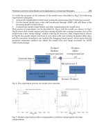
Fig. 3. DMCDM architecture with receding horizon.
When I(z
-1
) is the convolution of two vectors: one array is product of h(z)·Spp, the second
array is Δ operator. Spp is new matrix calculated as Sp but using Markov coefficients of
disturbance of the system. More information is available at Thesis of Garcia[16].
4. Practical set up and experimental behavior
This chapter is presenting the author’s experience for tuning the algorithm. Also the steps
recommended for carry out a control solution. MBPC is a family on controller very suitable
for controlling systems in different conditions. They can consider constraints, control cost,
future information, model behavior etc Getting the model by linearization should be
considered. There are many identification algorithms, using the right ones and using the
best parameters can bring you success or failure.

Advanced Model Predictive Control

380
4.1 System identification
In control engineering ther are two important concepts that are opposite: Robustness and

Performance. Usually as much Robust is a controller as less Performance it offers you. So as
much Performance we demand as much easy to reach instable zones. There is one way to
get both characteristic at the same time, Model accuracy. If we have a better model or a more
accurate model, we will be able to demand more performance and more Robustness. So the
system model is one of the most important topics in control engineering.
The most famous PID control tuning techniques are Ziegler-Nochols rules or Cohen-Coon
method. Methods have a main characteristic, you can tune a PID controller with Robustness,
but unfortunately performance is not good enough. The main reason for is that you have not
a system model. So the quality model is very poor, thus Robustness is more important than
performance. When Performance is important, model quality must be improved. As good is
the model as good will be the control.
By other hand, the easiest way to get a model is by mean of physical equations. If we know
the physics of the system, by using physical equation we can obtain a very good quality
model. When physical equations are used model reach an important complexity, sometimes
the computational effort done by the microcontroller or commuter is very high. Some
models need mode than two day for calculating few second of real physical behavior.
An important approach use to be linear model. The computational cost of linear model, use
to be very low (few micro seconds every step time). Additionally much real system use to
have a linear behavior, so linear approach, sometimes, is the most intelligent solution. When
system has a non-linear behavior other solutions can be approached. Linearization is a good
solution for that.
When physical equations are hard to compute, linearization of them bring us a model easy
to carry out and fast to be calculated. Another solution is linear model by identification
techniques. When identification is our choice this kind of model works very well in the
identified point and around of it, but we have problems when the operating point is too far
from the identification point. When this problem appears a new linear model can be
identified. We can do this topic as many times as we need. Thus we apply a technique
similar to gain schedule but with models.
The main advantages of liner models are:
It is a simpler, so you have an easier solution for solving Differential equations.

The system behavior can be observed.
Any kind of order can be used. We should fit the order to the one system expected.
As disadvantages we can find:
The solution is exact, only in the operating pint and good enough close to it, but it is not
good as far as we are.
Experimental data is needed and sometimes particular experiments are not possible to carry
out.
No physical sense in poles and zeros identified can be found.
Math of the transfer functions, state space model and other can be studied in Ogata
continuous , Ogata Discrete or Zhu [43] books. Additionally some identification algorithms
were tested and studied widely in bibliography.
Lineal model available in bibliography:
Markov coefficients or impulse response model, there is an equivalent model, the step
response.
ARX: autoregressive with exogenous variable. ARMAX: Autoregressive moving average
with exogenous variable. OE: Output error. BJ: box Jenkins. CARIMA or ARIMAX:
MBPC – Theoretical Development for
Measurable Disturbances and Practical Example of Air-path in a Diesel Engine

381
autoregressive integral moving average with exogenous variable. State space models
deterministic, advanced and stochastic ones etc. all models are descried in Garcia [17].
Finally the solution proposed is linear models by sections. When linear model is valid, then
it shall be used, when linear model is not valid a new linear model must be placed.
4.1.1 Experimental data for identification
Many times data available is not a suitable data for identification. That is why system is
working and particular experiments are not allowed. Thus a measurement of system behavior
should be done and transient data must be used in the identification. Steady data does not
include important dynamic information, so transient contains the system dynamics.
When particular experiments can be done, they must be well chosen. An easy experiment

use to be a step applied to the system. The step should contain some characteristics:
powerful enough, long enough, the response must be in the linear zone. Theoretically white
noise is the best signal. But some authors, as Luo[22] or Zhu[43], studied physical inputs
and pseudo aleatori input is the best choice.
Some times a simple step or impulse can be applied and Strejc, Csypkin methods can be
applied. Simple model is obtained and some time it is good enough. Frequency
identification methods are also available, based in bode diagram or graphical techniques.
Identification algorithms are proposed in this chapter. Experimental data must be pre
processed and model structure should be well chosen. Parametrical and state space
identification can be carried out.
When parametrical identification is proposed the following steps should be respected:
1.
Experimental identification design and data acquisition.
2.
Data pre processed: filtering, remove data tends, data normalization etc.
3.
definition of model structure.
4.
Identify the model by using an appropriate identification algorithm.
5.
Studying model proprieties (zeros, poles, gain, … ) and model validation.
6.
If the model is the expected one, this task is finished, else come back to step 1, 2 or 3,
depending on problems detected.
4.1.2 Identification algorithms
The identification algorithms proposed and tested in this work is the PEM (Prediction error
method). Other where tested N4SID (Numerical Algorithm for Sub Space State System
Identification) widely explained in [108,141,150]. Bud PEM is preferred by this author with
very well results. PEM is an identification algorithm of state space model, so this model
should be converted in a equivalent transfer function.

4.1.3 System identification
A Diesel engine is identified. Some experimental data is shown. At this studied case air path
or air management system is going to be controlled. If suitable linear models cannot be
found, algorithms based on the Hamertein and Wiener models [12] can be used or non
linear models. The disadvantages of this latter group are: high computational cost and the
difficulty of programming them in a commercial ECU (electronic control unite).
The system air-path in a Diesel engine consists on controlling VNT (variable nozzle turbine)
in order to keep boost pressure in the set point. The engine controlled is a Diesel engine of
heavy duty applications, see figure 4. This is a truck engine, where EGR system is not

Advanced Model Predictive Control

382
included but VNT is available. Air-path is influenced by mass fuel injected, as much fuel
injected into cylinder, more power available in the turbine and more boost pressure. Fuel
injected is available information in the ECU.


Fig. 4. System controlled.
Unfortunately the fuel injected is selected by user’s needs. Thus fuel injected can not be
controlled by control algorithms and it is determined as a measurable disturbance.
Experimental identification done is in figure 5.


0 40 80 120 160 200
Time
(
s
)
40

80
120
160
200
240
mf (mm
3
/stroke)
0
20
40
60
80
100
PWM (%)
1000
1250
1500
Engine speed (rpm)

Fig. 5. Identification test performed at 1200 rpm. PWM signal is the control action on the
VNT, and mf is the injected fuel. Important variations in the engine speed are due to the
dynamometer response.
MBPC – Theoretical Development for
Measurable Disturbances and Practical Example of Air-path in a Diesel Engine

383
The VNT input applied can be seen in figure 6, where pseudo-random PWM (Pulse Width
Modulation PWM) is applied in the VNT. Aleatori fuel is injected in the engine. With these
inputs the boost pressure response is shown in figure below:

0 40 80 120 160 200
Time(s)
1
1.5
2
2.5
Boost p
r
essu
r
e (ba
r
)

Fig. 6. Boost pressure response.
Apparently these data have not any kind of relation, but continuing with identification process
we can obtain a system model. As shown the model poles are two. Physical systems don’t use
to have more than three poles, when model is bigger than this we could find some problems,
identification algorithm tried to identify signal noise, and it has identified fast poles.
()
55
54
44
1,7.10 5,1.10
0,983 -0,022 0,008
0,016 0,886 0,115 ; 5.8.10 5.10
0,002 0,027 0,907
2,1.10 5.10

8,89 1,18 1,2 ; 0
AB
CD
−−
−−
−−

−−




==−



−−

−


=−−=

Checking the results, we could realize that the system model is good enough, see figure 7.


04080120160200
T
i
(

)
-0.5
0
0.5
Boost pressure variation (bar)

Fig. 7. Measured evolution (black) and predicted evolution (grey) of the boost pressure for
the validation test at 1200 rpm.

Advanced Model Predictive Control

384
4.2 Control system examples
Once the model is identified the controller is calculated by using control algorithms
developed in section 3, it is time to control the system and testing with experimental data. A
comparison is going to be shown in the following figures. The test proposed is a transient
from steady conditions to full load. This is a typical situation in which a Diesel engine is
requested full load to make advancement in a road. The engine is turning at 1200 rpm and
no torque is need, suddenly all torque available is needed, and then engine, electronics and
thermodynamics must change to the new conditions. Four different algorithms are
controlling the system. The idea is testing those algorithms in order to check the engine
behavior if the controller of air path is one algorithm or other one.
The algorithms tested were: PID controller with feed forward of fuel behavior, PID with
Fuzzy login in parameters plus feed forward in fuel injected, GPCDM developed before and
DMCDM shown in section 3.
PID controller was tuned for getting the best feasible performance. It was tuned from
Ziegler Nichols parameter to updating PID until the performance was good enough. Feed
forward was programmed to use measurable disturbance behavior available.
PID Fuzzy: this controller was programmed as one improvement of standard PID. The
proposed algorithm is a gain schedule depending on error. Feed forward is also used here.

DMCDM: a model predictive controller based on impulse response with measurable
disturbance. Control horizon and prediction horizon are chosen as long time. When
performance is required long control horizon and prediction horizon must be chosen. Fro
tuning the algorithm one weight is fixed to 1 and the other is changed.
GPCDM: this is an other MBPC, so many ideas explained for DMCDM are applicable here.
Long time control horizon and long time prediction horizon are used for reaching good
performance. The real control cost is not available, so we keep one weight fixed and we fit
the second weight for tuning the system. GPC and GPCDM have a very special parameter,
which is not in other kinds of MBPC. T polynomial is a parameter, which theoretically is a
polynomial with zeros of the colored derivative noise from CARIMA model. In fact, it is a
parameter for tuning the GPC. When noise is present in the system, this parameter must be
tuned else you could put it as 1. there are many works explaining the behavior of the
parameter Clarke [26]. Moreover the robustness of the system is widely improved by tuning
the parameter [28,132]. Typical values of T polynomial are T= 1-0,7*z
-1
; or T = convolution of
( [1-0,7.z
-1
],[ 1-0,7.z
-1
]), sometimes 0,7 are placed by 0,8 or 0,6. This is an empirical rule that
can help the designer to choose the best option.
The structures are programmed as follow:
PID feed forward:
The boost pressure set point is depending on engine speed and mass fuel requested by used.
Additionally the fuel injected is the measurable system disturbance. So the fuel injected is
the feed forward control action. Error between boost pressure set point and measured boot
pressure is the input to the PID controller. Control action calculated is the addition between
feed forward and PID in figure 8. Finally control action applied is the calculated one
processed by one anti-windup. Experimental result will be shown in following figures.

The controller proposed and programmed in the figure 9 is similar architecture to the PID
proposed but some differences. The PID parameters are scheduled by a Fuzzy logic
technique. Other sub-systems are the same, PID, feed forward and anti-windup. The
behavior is similar to the PID but parameters can be tuned more accurate than a standard
PID controller. The main difficult in this controller is the tuning process, because the
MBPC – Theoretical Development for
Measurable Disturbances and Practical Example of Air-path in a Diesel Engine

385
parameters are more difficult to set up. The experience of the designer must be higher than
the standard PID. For tuning the controller many experiments must be done and widely
analyzed for choosing the best option.




Fig. 8. PID Architecture programmed.




Fig. 9. PID scheduled by fuzzy controller and feed forward.
GPCDM architecture is the one proposed in the figure 10. Set point is processed by h(z).
when future set point is not available, future ones are the actual one. Thus h(z) became as a
constant term. Additionally measurable disturbance can be processed as past information


Advanced Model Predictive Control

386

Fig. 10. GPCDM programmed.
and future information, see equation (30). In this experiment only actual and past fuel
injected can be processed, but future disturbances can be considered. Anti-windup is also
programmed, when control action calculated is higher than maximum, the algorithm is
frozen. Thus the integral component of the algorithm can not affect to the algorithms
performance.




Fig. 11. DMCDM programmed.
DMCDM programmed is shown in figure 11. Measurable disturbances are considered and
included in the controller. Anti-windup is programmed, a similar system to the one used in
the GPCDM. When maximum or minimum control action is reached, the algorithm is frozen
until control action is going to the opposite way.
MBPC – Theoretical Development for
Measurable Disturbances and Practical Example of Air-path in a Diesel Engine

387
5. Experimental results
As explained before full load transient test were done. The engine was in steady conditions
or idle conditions at 1200 rpm. When test starts, full load is required from the engine. Thus
maximum quantity of fuel is injected in order to burn it and getting the power. Additionally
air mass is needed for burning the fuel, which is why VNT must be controller to give the
boost pressure necessary for the new conditions. More boost pressure that necessary
produces an increment in exhaust pressure and some loses of torque and power and more
pollution in exhaust gases. If we have less boost pressure than set point then we will not
have enough air flow for burning the fuel in the right conditions.
Many experiments were done, but only the best performance is shown in this chapter. In

figure 12, boost pressure can be observed, figure 13 contains exhaust pressure behavior, and
the figure 14 shows engine torque.

5 7 9 11 13 15
Time (s)
1.2
1.4
1.6
1.8
2.0
2.2
2.4
2.6
2.8
3.
0
Boost P
r
essu
r
e (ba
r
)
Set Point
PID with Feed Forward
Fuzzy with Feed Forward
DMCDM
GPCDM

Fig. 12. Boost pressure evolution in transient conditions.

5 6 7 8 9 10 11 12 13 14 15
Time (s)
1.0
1.5
2.0
2.5
3.0
3.5
Exhaust P
r
essu
r
e (ba
r
)
PID
Fuzzy
DMC
GPC

Fig. 13. Exhaust pressure evolution in transient conditions.

Advanced Model Predictive Control

388
In figure 12, boost pressure behavior is presented. Thin line is the set point requested from
idle condition to full load one. This is the best boost pressure conditions considering,
efficiency, torque, power, pollution etc. so the system must be in set point as soon as
possible. Continuous lines are PID controller, solid red line is the PID with feed forward and

solid blue line is the PID Fuzy logic controller. GPCDM is the dashed blue line and
DMCDM is the dashed black line.
When transient test starts, the first part of the test are the same in all controllers. This
happens because VNT is in bounds, completely close and no different performance can be
appreciated. When VNT must be opened controller performance is different. GPCDM is
opening the VNT before than others, that is why over oscillation is lower than others. The
predictive model CARIMA helps the GPCDM to advance the system behavior, thus
GPCDM can predict the VNT open to be before and avoiding the over oscillation. PID must
be tuned with low influences of derivative term, the reason is the stability. Derivative term
can produce instable conditions in the system. This controller realizes later about over
oscillation and start opening the VNT later. The worst performance is done by DMCDM.
Maybe the system model is very single and it is more sensible to non-linearity. Fuzzy
controller improves the PID behavior because it is an improvement of PID.
Figure 12. contains the exhaust boost pressure. The steady conditions are reached in similar
time to boost pressure. The over-pressure in exhaust produces over-speed in turbine or
torque loses, and more pollutants than permitted.

5 7 9 11 13 15
Time (s)
0
300
600
900
1,200
1,500
1,800
2,100
2,400
Torque (N.m)
PID

Fuzzy
DMC
GPC
6 7 8 9 10 11
Time (s)
1,800
1,900
2,000
2,100
2,200
Torque (N.m)
PID
Fuzzy
DMC
GPC

Fig. 14. Torque evolution and air-path influence during transient.
MBPC – Theoretical Development for
Measurable Disturbances and Practical Example of Air-path in a Diesel Engine

389
Figure 14. shows torque performance. Both GPCDM and Fuzzy reach steady conditions at
the same time. So the torque is not very influenced by boost pressure. But if other controllers
are analyzed engine torque is influenced and oscillations are very uncomfortable.
Finally a summary of system response are shown in table 1 and table 2. Table 1 summarizes
the system response from the point of view of engine analysis. Table 2 analyzes the system
from the point of view of control parameters.

Experimental results

Max
Exhaust
pressure
(bar)
Overshoot
Exhaust
pressure
from steady
conditions
max
(Exhaust
Pressure) -
max(Boost
Pressure)
Max(Torque)
Torque
overshoot
PID+FF
3.223 53.48 0.482 2031 85
PID+FF+Fuzzy
3.443 63.48 0.702 2100 86
DMCDM
3.220 53.33 0.428 2101 133
GPCDM
2.655 26.43 0.129 2055 36
Table 1. Experimental results of system behavior.

Experimental results

22.5

2
5.5
()et dt⋅


22.5
2
5.5
udtΔ⋅


J
Boost
pressure
overshoot
PID+FF
29.11 454.38 51.83 34.10
PID+FF+Fuzzy
29.13 2911.15 174.68 33.10
DMCDM
36.96 18.80 37.90 39.20
GPCDM
27.62 37.40 29.49 12.60
Table 2. Experimental results, control parameters.
The most important variable from the point of view of control is the control Cost or J. This
variable summarized the control behavior from the point of view of control cost,
considering control effort and control error.
5.2 Discussion
The first conclusion that can be drawn from analyzing the results is that when fuel mass is
considered in the algorithm, behavior is always improved. This fact had been observed

during the identification process and is logical, since the more information the algorithm has
about the system, the better control it can apply. This is due to the air management process
being more influenced by fuel amount than VGT control actions. The fuel amount gives
energy, this energy goes to the turbine and the turbocharger increases its speed, thus the air
management system changes. The delivered fuel quantity therefore has a very strong
influence on the air management system. If this variable is included in control algorithms,
better control will be obtained.
The analysis of the behavior of the Fuzzy controller seems to show quite a good response
but at the cost of a high control effort. One of the disadvantages of this type of controller is

Advanced Model Predictive Control

390
the high overshoot of the exhaust pressure. The control effort is one order of magnitude
higher than the baseline controller. However, the greatest disadvantage is their complicated
tuning process due to having a large number of independent parameters.
Another interesting aspect is that not all the MPCs work better than the existing controllers.
For example, the DMC provided rather doubtful results. This was a surprise and could be
explained as follows: the prediction model of the DMC is considered to be highly sensitive
to nonlinearities in the system, since the system itself is highly nonlinear (in spite of having
linear zone models). This algorithm finds it difficult to predict engine behavior and
therefore does not take the right decisions. However, the predictive control GPC algorithm
is based on the CARIMA model and is more robust to system nonlinearities. In fact, one of
the most important parameters for the correct GPC tuning was the polynomial T(z).
The best all-round algorithm was the GPCDM. The most significant difference between
algorithms can be seen in the exhaust pressure in Figures 8 and 9. This parameter indicates
the effort made by the engine to control the air path and high pressure has a negative
influence on engine torque.
The air management system, and consequently various engine parameters, was strongly
influenced by the controller used. One of the most susceptible to this influence is PMEP,

which also affects engine torque, turbocharger pressure, etc. If an overshoot occurs it will
produce exhaust pressure peak and pumping losses. This fact produced less efficiency and
torque during transient conditions.
6. Conclusions
Few linear models were obtained from the air management system of the engine and they
are quiet good approximations of the nonlinear plant. These models can be used for linear
controller design with low computational effort. GPCDM, DMCDM, PID and Fuzzy PID are
tested in a standard test bench. In comparison to standard gain scheduled PID, setpoint
tracking could be improved. The additional degrees of freedom of GPC can be used for
tuning the robustness of control.
7. Acknowledgements
I would like to thank Universidad Jaume I from Castellon (Spain). I am assistant professor in
the engineering department. Moreover I want strongly thank Vinci Energia. In this company
Ia m working as a professional researcher and many of the improvements in control theory
are applied to solar tracking system in my actual investigations. And of course, this work
was impossible to do without CMT thermal engines of the “Universidad Politécnica de
Valencia”.
8. References
[1] Albertos P. y Ortega R. “On generalized predictive control two alternative formulations”.
Automatica, Vol. 25 No.5, pp. 753–755, 1989.
[2] Bordons C. y Camacho E.F. “A generalized predictive controller for a wide class of
industrial process”. IEEE Transactions on control system technology, Vol. 6 No. 3,
May 1998.
MBPC – Theoretical Development for
Measurable Disturbances and Practical Example of Air-path in a Diesel Engine

391
[3] Camacho E.F., Berenguel M. y Rubio F.R. “Application of a Gain Scheduling Generalized
Predictive Controller to a Solar Power Plant”. Control Engineering Practice, Vol.
2(2), pp. 227–238, 1994.

[4] Chow C. y Clarke D.W. “Actuator nonlinearities in predictive control advances in model-
based predictive control”. Ed. Oxford university press, p´ag. 245, 1994.
[5] Clarke D.W. y Gawthrop P.J. “Self-tuning controller”. Proc. IEE, Vol. 122, pp. 929–934,
1975.
[6] Clarke D.W. y Gawthrop P.J. “Self-tuning control”. Proc. IEE, Vol. 126, pp. 633–640, 1979.
[7] Clarke D.W. yMothadi C. “Properties of generalized predictive control”. Automatica,
Vol. 25(6), pp. 859–875, 1989.
[8] Clarke D.W., Mothadi C. y Tuffs P.S. “Generalized predictive control -Part I. The basic
algirithm”. Automatica, Vol. 23 No.2, pp. 137–148, 1987.
[9] Clarke D.W., Mothadi C. y Tuffs P.S. “Generalized predictive control -Part II. Extension
and interpretation”. Automatica, Vol. 23 No.2, pp. 149–160, 1987.
[10] Clarke D.W. y Zhang L. “Long-range predictive control using weightingsecuence
models”. IEE Proceedings, Vol. 134 D No.3, 1987.
[11] Corradini M.L. y Orlando G. “A VSC algorithm based on generalized predictive
control”. Automatica, Vol. 33 ,5, pp. 927–932, 1997.
[12] Cutler C.R. y B.L. Ramaker. “Dynamic matrix control–a computer control algorithm”.
Proceedings of the Joint Automatic Control Conference, 1980.
[13] de la parte M. Perez, Camacho O. y Camacho E.F. “Developement of a GPC-based
sliding mode controller”. ISA Transaction, Vol. 41 No.1, pp. 19–30, 2002.
[14] Evans W.R. “Control system synthesis by root locus method”. AIEE Transaction, Part II,
Vol. 69, pp. 66–69, 1950.
[15] Galanti M., Magrini S., Mosca E. y Spicci V. “Receding horizon predictive control
applied to a high performance servo-controlled pedestal”. Proc. of ESPRIT (III
workshop on industrial application of MBPC, Cambridge, 1992.Soeterboek R.
Predictive control a unified approach. Prentice Hall int. UK Cambridge, 1992.
[16] Garcia C.E. y Morshedi A.M. “Quadratic programming solution of dynamic matrix
control (QDMC)”. Chemical engineering communication, Vol. 46, pp. 73–87, 1986.
[17] García-Ortiz, J.V. “Aportación a la mejora del control de la renovación de la carga en
motores Diesel Turboalimentados mediante distintos algoritmos de control”. Thesis
in Universidad Politécnica de Valencia. CMT Motores térmicos. 9 Julio 2004.

[18] Havlena V. y F.J. Kraus. “Receding horizon MIMO LQ controller design with
guaranteed stability”. Automatica, Vol. 33 No.8, pp. 1567–1570, 1997.
[19] Kennel R. “Generalized predictive control GPC-ready for use in drive application?”.
32nd IEEE electronics specialist conference PELS Vancouver June, 2001.
[20] Keyser R.M.C. De, de Velde G.A. Van y Dumortier F.A.G. “A comparative study of self-
adaptative long-range predictive control methods”. Automatica, Vol. 24(2), pp.
149–163, 1988.
[21] Kouvaritakis B., Cannon M. y Rossiter J.A. “Who needs QP for linear MPC anyway?”.
Automatica, Vol. 38, pp. 879–884, 2002.
[22] Kouvaritakis B., Rossiter J.A. y Chang A.O.T. “Stable gerenalized predictive control: an
algorithm with guaranteed stability”. Proc. IEE, Part D,, Vol. 139(4), pp. 349–362,
1992.
[23] Luo X. Analysis of automatic control system for deposition of CIGS films. Tesis
Doctoral, Colorado School of Mines, Colorado Illinois, USA, 2002.

Advanced Model Predictive Control

392
[24] Martinez M., Senent J. y Blasco X. “A comparative study of classic vs genetic algorithms
optimization applied in GPC controller”. IFAC world congress, San Francisco USA,
1996.
[25] Mosca E. y Zhang J. “Stable redesign of predictive control”. Automatica, Vol. 28, pp.
1229–1233, 1992.
[26] Nuñez A., Cueil J.R. y Bordons C. “Modelado y control de una almazara de extraccion
de aceite de oliva”. XXII Jornadas de Autimatica, 2001.
[27] Nyquist H. “Regeneration theory”. Bell system tech. Journal, Vol. 11, 1932.
[28] Overschee P. Van y Moor B. De. “N4SID: Subspace algorithm for the identification of
combined deterministic-stochastic systems”. Automatica, Vol. 30, pp. 75–93, 1994.
[29] Pannocchia G. y Rawlings J.B. “Robustness of MPC and Disturbance Models for
Multivariable Ill-conditioned Processes”. Technical report TWMCC No. 2001-02,

2001.
[30] Poulser N.K., Kuovaritakis B. y Cannon M. “Constrained predictive control and its
application to a coupled-tanks apparatus”. Int. Journal of control, Vol. 74 No. 6, pp.
552–564, 2001.
[31] Qin S.J. y Badgwell T.A. “An overview of industrial model predictive control
technology”. AIche symposium series, Vol. 316(93), pp. 232–256, 1996.
[32] Qin S.J. y Badgwell T.A. “A survey of industrial model predictive control technology”.
Control engineering practice, Vol. 11, pp. 733–764, 2003.
[33] Richalet J., Rault A., Testud J.L. y Papon J. “Model predictive heuristic control:
Applications to industrial processes”. Automatica, Vol. 14, pp. 413–428, 1978.
[34] Salcedo J.V, Martinez M., Sanchis J. y Blasco X. “Design of GPC’s in state space”.
Automatika, Vol. 42(3-4), pp. 159–167, 2001.
[35] Sanchis J., Martinez M., Ramos C. y Salcedo J.V. “Principal component GPC with
terminal equality constraint”. In 15th IFAC World Congress , Barcelona (Spain),
July 2002.
[36] Shridhar R. y Cooper D.J. “A tuning strategy for unconstrained SISO model predictive
control”. Ind. Eng. Chem Res., Vol. 36, pp. 729–746, 1997.
[37] Soeterboek A.R.M., Verbrugger H.B., der Bosch P.P.J Van y Butler H. “Adaptative
predictive control-A unified approach”. Proc. 6th Yale workshop on applied of
adapt. system theory new Haver USA, 1990.
[38] Soeterboek A.R.M., Verbrugger H.B., der Bosch P.P.J Van y Butler H. “On the
unification of predictive control algorithm”. Proc. 29th IEEE conference on decision
and control, Honolulu USA, 1990.
[39] Soeterboek R. Predictive control a unified approach. Prentice Hall int. UK Cambridge,
1992.
[40] Tsang B.A. y Clarke D.W. “Generalized predictive control with input constraints”. IEE
Proceedings, Vol. 135, 1988.
[41] Verhaegen M. “Identification of the deterministic part of MIMO state space models”.
Automatica, Vol. 30, pp. 61–74, 1994.
[42] Zafirion E. “Robust model predictive control of process with hard constraints”. Comp.

Chen. Eng., Vol. 14, pp. 359–371, 1990.
[43] Zheng A. y Morari M. “Stability of model predictive control with soft restraints”.
Proceedings 33rd CDC Florida, pp. 1018–1023, 1994.
[44] Zhu Y. y Backx T. Identification of multivariable industrial process, for simulation,
diagnosis and control. Springer-verlag, ISBN 3-540-19835-0, 1993.
18
BrainWave
®
: Model Predictive Control
for the Process Industries
W. A (Bill) Gough
Andritz Automation Ltd.
Canada
1. Introduction
This chapter describes the development and application of a model-based predictive
adaptive (MPC) controller, commercially known as BrainWave®. This controller is a
patented (US Patents #5,335,164 and #6,643,554) PC-based commercial software package
with hundreds of installations around the world in many different process industries. The
predictive control capability enables significant performance improvements compared to
manual or other automatic control strategies for processes with long time delays or multi-
variable interactions. Process variability reductions of 50% or more are typically achieved
using this technique.
MPC technology has been used for many years in the petroleum industry but it is not yet
common practice in most industries. The high cost and implementation complexity have
been barriers to the wide spread use of MPC. It is therefore important that an MPC tool be
designed for ease of use to reduce the cost of installation and life cycle maintenance. Model
identification and controller tuning are the primary tasks involved in the installation of an
MPC controller so the controller must be designed to make these functions as easy as
possible. The controller should be designed to handle self-regulating systems, open loop
unstable (integrating) systems, and multivariable systems, so that the one controller can be

used to solve as many applications as possible, avoiding the need for the user to learn and
support too many different controller designs.
BrainWave is an MPC controller that has been developed to solve the most common types of
difficult regulatory control problems. It has been deployed in a wide variety of process
industries including pulp & paper, mineral processing, plastics, petrochemicals, oil and gas
refining, food processing, lime and cement, and glass manufacturing. BrainWave is
designed for ease of use. A novel process identification and modeling method based on the
Laguerre series transfer function helps to simplify the steps required to obtain a model of
the process response. Internal normalization techniques simplify the setup and tuning of the
controller. BrainWave is designed to control processes that are self-regulating, integrating,
or multivariable, so this one MPC tool can be used for virtually all difficult regulatory
control loops in a plant.
The chapter will describe the mathematics behind the Laguerre modeling method, and show
the development of the predictive control law based on the Laguerre state space model used
in the BrainWave controller. The user interface from the actual software implementation will
be illustrated. Several application examples from the Pulp & Paper and Mineral Processing

Advanced Model Predictive Control

394
industries will be provided that highlight the different types of regulatory control problems
where MPC provides clear advantages over conventional PID type loop controllers.
2. Adaptive model-based predictive controller development
Obtaining a process response model is a key part of the implementation of an MPC
controller. In our design, the controller models the system response using a generic function
series approximation technique based on Laguerre polynomials. This approach provides a
simple and efficient method to mathematically model the process response with a minimum
of a priori information. It also enables the controller to perform online adaptation of the
process response models automatically. These factors reduce the implementation effort and
contribute to quick installation times. The adaptive capabilities assist the control technician

with developing the process response models, and the default configuration of the control
parameters ensures excellent control performance once the process model is obtained. These
features help to ensure the same good result will be achieved regardless of the expertise
level of the person doing the application. For industrial customers that operate large plants
with thousands of process controllers, this benefit alone is extremely valuable.
Using these models as the basis for a predictive control design, the MPC is able to control
processes with long delay or response times (or fast response processes where the time
delay is a significant part of the response dynamics) better than is possible using PID type
controllers. This technique can also be used to automatically model and counteract the
effects of measured disturbances by incorporating them into the control strategy as feed
forward variables. The use of feed forward variables is particularly important for long time
delay systems so that disturbances can be cancelled much sooner than is possible using
feedback control alone.
The advanced process control algorithm presented here is an adaptive model-based
predictive controller that has its origins in the work of (Zervos & Dumont, 1988). They
proposed the use of a state-space model derived from Laguerre orthogonal basis functions
so that adaptive control could be achieved without the need to know the process order or
the time delay in advance. This approach reduces the a priori knowledge required to develop
a high fidelity model of the process transient response, thus simplifying the modeling task.
An analogy to this method is the use of Cosine functions in the Fourier series method to
approximate periodic signals as is common in frequency analyzers. In this case, weights for
each Cosine function in the series are determined such that when the weighted Cosine
functions are summed, a reasonable approximation of the original signal is obtained. In this
case the signal is represented by its frequency spectrum, with each basis function weighting
coefficient representing the contribution of each frequency present in the original signal.
This method is efficient due to the similarity of the basis functions in the series to the signal
being modeled, and also due to the special mathematical property of the basis functions
called orthogonality that ensures the unique solution of the basis function weighting
coefficients in the identified model.
In process control, the process transfer functions are transient in nature and are not periodic,

so Cosine functions are not an appropriate choice as a basis for the model. However, the
elegance of the Fourier series technique provides many advantages such as simple and
efficient model structure and excellent parameter convergence when estimating the model
from observed data sets due to the orthogonality property of the Fourier series. The
motivation of this research was to find an equally simple and efficient method to model the
transient responses common in process control applications.

BrainWave®: Model Predictive Control for the Process Industries

395
The Laguerre functions are well suited to modeling the types of transient signals found in
process control because they have similar behavior to the processes being modeled and are
also an orthogonal function set. In addition, the Laguerre functions are able to efficiently
model the dead time in the process response compared to other suitable function sets. This
Laguerre model is used as a basis for the design of the predictive adaptive regulatory
controller.
Laguerre basis functions are defined by:

()
()
()
()
()
1
1
1
exp
2exp2
1!
i

i
i
i
pt
d
Lt p t pt
i
dt
−
−
−
=−
−
(1)
Where L
i
is the i
th
Laguerre function, and p is a scaling parameter referred to as the Laguerre
pole.
Each Laguerre basis function is a polynomial multiplied by a decaying exponential so these
basis functions make an excellent choice for modeling transient behavior because they are
similar to transient signals. For use in modeling processes, these basis functions are written
in the form of a dynamic system. With appropriate discretization (assuming straight lines
between sampling points), the orthogonality of the basis functions is preserved in discrete
time.
Summing each Laguerre basis function with an appropriate weighting factor approximates a
process transfer function:

gt cl t

ii
i
i
() ()=
=
=∞

0

(2)

The Laguerre function has the following Laplace domain representation:

1
()
( ) 2 , 1, ,
()
i
i
i
sp
sp i N
sp
L
−
−
==
+
(3)
where: i is the number of Laguerre filters (i = 1, N);

p > 0 is the time-scale;
L
i
(s) are the Laguerre polynomials.
The reason for using the Laplace domain is the simplicity of representing the Laguerre
ladder network, as shown in Fig. 1.

U(s)
2 p
sp+
L
1
(s)
sp
sp
−
+
L
2
(s)
sp
sp
−
+
L
N
(s)
C
1
C

2
C
N
Y(s)
Summing Circuit

Fig. 1. Laguerre ladder network

Advanced Model Predictive Control

396
This network can be expressed as a stable, observable and controllable state space form as:

(1) () ()lk Alk buk+= + (4)

() ()
T
y
kclk= (5)
where:
[]
1
( ) ( ), , ( )
T
T
N
lk l k l k= is the state of the ladder (i.e., the outputs of each block in Fig. 1);
[
]
1

( ) ( ), , ( )
T
kN
Ck ck ck= are the Laguerre coefficients at time k;
A is a lower triangular square (N x N) matrix.
The Laguerre coefficients C(k) represent a projection of the plant model onto a linear space
whose basis is formed by an orthonormal set of Laguerre functions.
The same concept used in the plant identification is used to identify the process response for
measured feed forward variables. For unmeasured disturbances, an estimate of the load is
made. This estimate is based on the observation that an external white noise feeds the
disturbance model, resulting in a colored signal. The disturbance can be estimated as the
difference between the plant process variable increment and the estimated plant model with
the integrator removed. Using the plant and disturbance models we can then develop the
Model Predictive Control (MPC) strategy.
The discrete state space model used by Zervos and Dumont for the control design takes the
(velocity) form:

1
1
kkk
kk k
u
yy
+
−
Δ=Δ+Δ
=+Δ
xAxb
cx
(6)

Where
u is the input variable, which is adjusted to control the process variable
y
and x is
the n
th
-order Laguerre model state. The subscript k gives the time index in terms of number
of controller update steps; so the
Δ
operator indicates the difference from the past update.
For example,
1kkk−
Δ= −xxx
. The n×n matrix
A
and the n×1 matrix b have fixed values
derived from the Laguerre basis functions. Values of the 1×n matrix
c are adjusted
automatically during model adaptation to match the process model predictions to the actual
plant behaviour. The dimension n gives the number of Laguerre basis functions used in the
process model. The algorithm presented here does not suffer from over parameterization of
the process model. The BrainWave controller uses n=15, which has proven to be enough to
model almost any industrial plant behaviour.
Notice that the state equation recursively updates the process state to include the newest
value of the manipulated variable. Therefore, we can view the process state as an encoded
history of the input values.
Model adaptation may be executed in real time following the recursive algorithm of
(Salgado et al, 1988). This algorithm updates the matrix
c
according to:

()
1
1
TT
kk
kk kkk
T
kk k
y
α
+
Δ
=+ Δ−Δ
+Δ Δ
Px
cc cx
xP x
(7)
Where the covariance matrix
P evolves according to:

BrainWave®: Model Predictive Control for the Process Industries

397

2
1
1
1

T
kkkk
kk k
T
kk k
α
β
δ
λ
+
ΔΔ
=− +−
+Δ Δ
Px xP
PP IP
xP x
(8)
I is the identity matrix. The constants
α
,
λ
,
β
and
δ
are essentially tuning parameters
that can be adjusted to improve the convergence of the adapted Laguerre model
parameters
C.
The value of the manipulated input variable u (the controller output) that will bring the

process to set point ( SP ) d steps in the future may be calculated using the model equations.
The formula for the process variable d steps in the future is:

()()
11dd
kd k k k
y
yu
−−
+
=+ ++ Δ+ ++ ΔcA IAx cA Ib
(9)
Since it is desired to have the process reach set point d steps in the future, we set
kd kd
ySP
++
= and solve for the manipulated input variable
k
uΔ .

()
()
1
1
d
kd k k
k
d
SP y
u

−
+
−
−− ++ Δ
Δ=
++
cA IA x
cA Ib


(10)
This equation is the basic control law. As with most predictive control strategies,
implementation of the strategy involves calculating the current controller output,
implementing this new value, waiting one controller update period, and then repeating the
calculation.
Predictive feed forward control can easily be included in this control formulation. A state
equation in velocity form is created for the feed forward variable:

1k
ff
k
ff
k
v
+
Δ=Δ+ΔzAzb (11)
Where z is the feed forward state and
v is the measured feed forward variable. The effect of
the feed forward variable is then simply added to the output equation for the process
variable to become part of the modeled process response:

1kk k
ff
k
yy
−
=+Δ+Δcx c z (12)
Notice that the feed forward state equation creates an encoded history of the feed forward
variable in the same way that the main model state equation encodes the manipulated
variable.
Re-deriving the control law from the extended set of process model equations yields:
()()()
()
11 1
1
dd d
kd k k
ff ff ff
k
ff ff ff
k
k
d
SP y v
u
−− −
+
−
− − ++ Δ− ++ Δ+ ++ Δ
Δ=

++
cA IA x c A IA z c A Ib
cA Ib
 


(13)
The basic structure of this control law does not change as additional feed forward variables
are included in the process model, so it is a simple exercise to include as many feed
forwards as necessary into this control law.

Advanced Model Predictive Control

398
Use of the Laguerre process model implicitly assumes that a self-regulating process is to be
modeled. In cases where a process exhibits integrating behaviour, it is necessary to modify the
Laguerre process model. The modification is two-fold. First, the Laguerre model is altered so
that the Laguerre state gives the change in the slope of the process response. That is:

1
1
1
kkk
kk k
kk k
u
yy
yy y
+
−

−
Δ=Δ+Δ
Δ=Δ +Δ
=+Δ
xAxb
cx (14)
Second, an unmeasured disturbance component is added to the model to estimate the
steady state load on the plant. The feedback control law is then derived based on the
modified Laguerre model, including the disturbance component.
The above gives the derivation of a d steps ahead adaptive model-based predictive
control for a single variable. Full multivariable processes (multiple-input, multiple-
output) may also be modeled using Laguerre state-space equations. However, to derive a
control law for the multivariable case it is preferable to optimize for a cost function such
as the one proposed in the generalized predictive control (Clarke et al, 1987), rather than
back calculating the control to achieve a d steps ahead outcome. This concept of predictive
control involves the repeated optimization of a performance objective over a finite
horizon extending from a future time (
N
1
) up to a prediction horizon (N
2
). Fig. 2
characterizes the way prediction is used within the MPC control strategy. Given a set
point
s(k + l), a reference r(k + l) is produced by pre-filtering and is used within the
optimization of the MPC cost function. Manipulating the control variable
u(k + l), over the
control horizon (
N
u

), the algorithm drives the predicted output y(k + l), over the
prediction horizon, towards the reference.
The control moves are determined by looking at the predicted future error, which is the
difference between the predicted future output and the desired future output (reference).
The user can specify the region over which these error values will be summed. The region is
bounded by the initial (N1) and final (N2) prediction horizon. It is also possible to set the
number of control moves that the controller will take to get to the set point by adjusting a
parameter called control horizon (Nu). If we weigh the predicted squared error from set
point and the total actuator movement with weighting matrices Q and R respectively, and
add the two sums, we arrive at the cost function employed within the BrainWave
Multivariable controller:


(15)
where Y (i), S(i) and U(i) are the predicted process response, the set point reference and the
controller output at update i, respectively. The tuning matrices Q and R allow greater
flexibility in the solution of the cost function. The above cost function is optimized with
respect to U. By differentiating and solving for U, the next set of optimal control moves is
obtained. Input constraints are implemented via a multivariable anti-windup scheme which
was proved to be equivalent to an on-line optimization for common processes (Goodwin &
Sin, 1984).

BrainWave®: Model Predictive Control for the Process Industries

399

Fig. 2. MPC control concept for multivariable applications
Once the cost function is built, it remains the same until we change one of the models, Q, R,
or one of the horizons. At each update, the following takes place: i) the state vector is
estimated and adjusted; ii) the process response is estimated, and iii) the next control output

is calculated.
Measured disturbances (feed forwards) are assumed to affect one process variable at a time.
There can be up to three measured disturbances per process variable in the current
controller software structure.
Aside from this change in the derivation of the control law, the multivariable algorithm is
substantially the same as the single variable algorithm. That is, a deterministic control law is
obtained which provides the current control move that will yield some future process
response, the current move is implemented, and then a new control move is calculated
based on new process data at the next control update step. For a complete mathematical
development of the control law used in the multivariable case, refer to (Huzmezan, 1998).
The controller outlined above has demonstrated more than twenty years of success in
industrial applications, verifying the effectiveness of this adaptive model-based predictive
control algorithm.
3. Commercial implementation of the BrainWave controller
The BrainWave MPC controller is commercially available as Windows based PC software.
The system connects to existing control systems using the OLE for Process Control (OPC)
standard interface. A communications watchdog scheme is used to ensure that the process
control automatically reverts to the existing control system in the event of any
communication or hardware faults associated with the BrainWave computer.
Despite the complex mathematics use in the control and model adaptation algorithms, the
software is designed to be easy to use and is suitable for control technicians to apply in an

Advanced Model Predictive Control

400
industrial setting. The user interface for the BrainWave system is shown in Fig. 3. The
interface includes a trend display of the process variables at the top right side of the
interface. In this example, the set point is the yellow line, the process variable is the red line,
and the controller output (the actuator) is the green line.
The identified process transfer function is shown on the lower right side. The transfer

function plot is generated based on a step input at time=0 and thus shows the open loop
transient response of the process to a change in the actuator or measured disturbance
variable. The white line is a plot of the estimated transfer function of the process (expressed
as a simple first order system using a dead time, time constant, and gain) which is used as a
starting point for the model identification. The red line is a plot of the identified process
transfer function open loop step response based on the Laguerre representation. The blue
bars represent the relative values of the 15 Laguerre series coefficients which are the
identified process model parameters.


Fig. 3. BrainWave user interface
BrainWave allows the user to configure single loop controllers (Multiple Input Single
Output – MISO) and multivariable controllers where more than one control loop interacts
with other control loops (Multiple Input Multiple Output – MIMO). The process type is
chosen as either self-regulating for stable systems or integrating for open loop unstable
systems such as level controls. The primary information required is an initial estimate of the
process response. This is entered using a simple first order plus dead time transfer function
estimate. This estimate is used by BrainWave to determine the appropriate data sample rate
for modeling and control of the process and also provides a starting point for the initial
Laguerre model of the process.

BrainWave®: Model Predictive Control for the Process Industries

401
Many systems are well described using the simple first order model estimate, and if the
estimate is reasonably close to the actual process response, the BrainWave controller will be
able to assume automatic control without any further configuration work. The default setup
parameters are set to values that will provide a closed loop response time constant that is
equal to the open loop response time constant of the process, thus providing effective and
robust control without any additional tuning required.

Multivariable MIMO systems can be configured with a dimension of up to 48 inputs and 12
manipulated outputs. Estimates of the response of each process variable to each actuator or
disturbance variable must be entered (if the cross coupling between the respective channels
exists) so the complete array of process transfer functions is shown as a matrix.
For MIMO systems, it is desirable to be able to place more priority on one process variable
than another as part of the controller setup. Similarly, some actuators are able to move more
quickly compared to other actuators. The MIMO control setup provides simple sliders that
allow the user to impose these preferences on the controller in a relative fashion between the
process variables and actuators. Note that the default settings provided will result in stable
and robust control of the process where the closed loop response time constant is equal to
the open loop response time constant for each process variable.
3.1 Model identification
The BrainWave controller has online modeling features that help the user obtain the correct
process transfer function model for the process. The model identification can be performed
in open loop by observing the process response to manual changes to the actuator(s) or in
closed loop during automatic control in BrainWave mode. Performing the model
identification in closed loop is advantageous as it allows the user to confirm the
improvement in the control performance at the same time as the convergence of the
identified model is monitored in the model viewer, thus providing real-time confirmation
that the identified process model is correct.
An example of the model identification procedure is shown in Fig. 4. The user starts by
entering an estimate of the process response in simple first order terms as described earlier
(the white line shown in the Model Viewer panel). BrainWave builds a Laguerre model that
matches this estimate and uses this model as a starting point for both the predictive control
operation and the model identification (the red line in the Model Viewer panel). A series of
set point changes are made while the BrainWave controller is in control of the process as
shown in the Trend display panel. Some overshoot is apparent during the first set point
change due to the errors in the initial process response estimate provided by the user. As the
series progresses, the identified process model converges to the correct value. As the model
becomes more correct, the control performance during each successive set point change is

improved. At the end of the sequence, the process model is completely converged to the
correct value, and the resulting control performance is ideal.
Feed forward disturbance variables can also be modeled automatically while BrainWave is
in control of the process. This unique capability allows the controller to identify the transfer
function of the disturbance variable to the process so that the controller can calculate the
correct control move with the actuator to cancel the predicted disturbance on the process.
This feature enables BrainWave to provide the best disturbance cancellation possible. An
example of the adaptive disturbance cancellation capability is shown in Fig. 5. The feed
forward variable is the square wave signal at the bottom of the figure. In this example, the

Advanced Model Predictive Control

402
BrainWave controller begins with no model for the feed forward disturbance variable so the
process is disturbed from the set point and the actuator (the trend in the center of the figure)
reacts by feedback after the disturbance has already occurred to return the process to the set
point. As the feed forward transfer function is identified by BrainWave, the controller
begins to take immediate action when the feed forward disturbance signal changes, thus
providing improved cancellation of the disturbance. As the identified feed forward model
converges to the correct value, the cancellation of the disturbance is complete.




Fig. 4. Process model identification during closed loop control

BrainWave®: Model Predictive Control for the Process Industries

403

Fig. 5. Adaptive feed forward disturbance cancellation
3.2 Predictive control
The identified process model is used as the basis to calculate the required control moves
with the actuator to bring the process to the set point some time in the future. For the single
loop MISO controller, the primary adjustment for control performance is the prediction
horizon. This is essentially the number of control steps into the future where the process
variable must be on the set point. A long prediction horizon results in conservative closed
loop control response; the actuator is simply positioned to the new calculated steady state
value and the process reaches the set point according to its natural open loop response time.
Shorter prediction horizons cause the controller to make a more aggressive transient move
with the control actuator in order to bring the process to the set point in less time than the
natural response. Fig. 6 shows the effect of adjusting the prediction horizon for self-
regulating (open loop stable) systems.
Fig. 7 shows the effect of adjusting the prediction horizon for integrating (open loop
unstable) systems. In addition to adjusting the prediction horizon, the set point reference is
also internally filtered to provide less aggressive actuator movement during set point
changes. It should be noted that integrating systems are only stable in closed loop for a
certain range of controller behavior (a marginally stable system in closed loop) so the
amount of arbitrarily fast or slow control performance adjustment is limited.
In the multivariable MIMO controller, there are several parameters that can be adjusted to
change the control performance. The weighting can be adjusted to change the penalty for set
point tracking error for each process variable and the movement penalty for each actuator.
The control horizon, which specifies the number of future control moves to be calculated,
can be made longer for conservative actuator movement and slower process response or
shorter for more aggressive actuator movement and faster process response. The prediction
horizon is also adjusted to determine the range of future process response that will be
included in the cost function minimization. Typically this range begins some time after the
0
10
20

30
40
50
60
70
80
1
47
93
139
185
231
277
323
369
415
461
507
553
599
645
691
737
783
829
Sample Number
Percent of Scale
Pr o c es s
Set Point
Actuator

Feed Forw ard
No Model
Adapted Model