Applications of High Tc Superconductivity Part 5 potx

Superconductivity Application in Power System
69




Fig. 27. IEEE 39 bus systems (HTS cable application: red line)
SI calculation of sample system
To consider power system reliability, N-1 contingency criteria was applied. Equation (3.1)
and (3.2) shows the severity index (SI, over load index and voltage index) used in ranking.
 Over-load index
Equation 3.1 represents over-load index.

2
max,
1
L
i
i
i
P
PI
P








(10)
 Voltage index
Consumption of reactive power can be known by voltage ranker which represents
increment of reactive power loss by increased load factor of line. Equation 3.2 represents
voltage index.

2
1
L
ii
i
PI X P



(11)
where
i
P
is active power,
i
X
reactance, and
max,i
P power ratings of i-line.
The results of SI on sample system results are shown in Table 3.4 and Table 3.5. As a result
of calculation, the first two contingency cases of each SI are determined as the object cases of
voltage stability calculation.

Applications of High-Tc Superconductivity

70

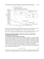
(a) before

(b) after
Fig. 28. P-V curve (HTS cable application)

Superconductivity Application in Power System
71
Rankin
g

No.
Contingency Line
PI[p.u.]
From Bus To Bus
1 21 22 10.8136-
2 23 24 8.6842
3 6 11 8.6463
4 13 14 8.6206
5 15 16 8.5228
Table 8. Performance index by line overload index

Rankin
g

No.
Contingency Line
PI[p.u.]
From Bus To Bus

1 28 29 10.8884
2 2 3 10.3888
3 16 21 10.2108
4 2 25 9.9931
5 6 7 9.8334
Table 9. Performance index by line voltage index of case I
Table 10 is the summary of the overloaded lines at severe contingency cases. HTS cable is
applied as the order of severity of overloaded line. The replaced system is shown as Fig.29.
Considered HTS cable constants are L = 0.10[uH/km], C=0.29[uF/km] respectly.
Incremented transfer capacity after HTS cable replacement is 8,880MW in base case and
5720MW in N-1 contingency case. Therefore, increased transfer capacity becomes 1820MW.

from to contingency rating flow overload(%)
16 24 OVRLOD 1 600.0 630.4 105.0
22 23 OVRLOD 1 600.0 665.5 107.9
23 24 OVRLOD 1 600.0 945.9 157.5
16 21 OVRLOD 2 600.0 681.0 111.3
21 22 OVRLOD 2 900.0 955.9 104.2
4 14 OVRLOD 3 500.0 566.2 113.7
10 13 OVRLOD 3 600.0 620.8 102.3
13 14 OVRLOD 3 600.0 636.3 105.5
6 11 OVRLOD 4 480.0 636.8 132.3
10 11 OVRLOD 4 600.0 618.2 102.1
Table 10. Overloaded lines at N-1 contingency
5.2 SFCL
In power system, proper SFCL application places are considered as (a)~(c) points of Fig. 29.
Point (a) is to limit fault current of distribution feeder. SFCL at (b) point reduces fault

Applications of High-Tc Superconductivity
72

current impact of adjacent transformer in case of parallel operation and protects bus bar.
Point (c) is general solution to reduce transformer secondary fault current and extend
Circuit Breaker changing time when distribution system experiences high fault current.


Fig. 29. SFCL application
6. Conclusion
The infrastructure of electric power system is based on conductor. With the change of power
industry, such as Kyoto protocol and Energy crisis, superconducting technology is very
promising one not only to increase efficiency of electricity but also to upgrade security of
power system. Among various superconducting technology, most applicable ones –HTS
cable, Fault current limiters, Dynamic SC are introduced and discussed how to apply.
Other superconducting facilities, like transformer, generator, SMES, Superconducting
Flywheel, are in testing and will be implemented with the changes of power market needs.
However, the most critical obstacle of power system application is superconductor material
and cooling system. Present HTS superconductors have to be improved much more than
conventional ones, but still have difficulties in general use, such as extreme low temperature
operation, hard manufacturing, AC loss and high cost. Cooling system is also hard task
which have close relation of HTS failure due to quench mechanism. In operating point of
view, monitoring and control to protect the local hot spot is another task to overcome.
More advanced superconductors and application methods are expected in power system
usage in near future.
7. Acknowledgment
Thanks to support all referenced paper authors and researchers in the field of superconductor
application in power system, especially Dr. OK-Bae Hyun and Si-Dol Hwang in KEPRI.

Superconductivity Application in Power System
73
8. References
Jon Jipping, Andrea Mansoldo, "The impact of HTS cables on Power Flow distribution and

Short-Circuit currents within a meshed network", IEEE 2001 O-7803-7285-9/01
M. Nassi, N. Kelley, P. Ladie, P. Coraro, G. Coletta and D. V. Dollen, "Qualification results of
a 50m-115kV warm dielectric cable system", IEEE Trans. on Applied
Superconductivity, Vol. 11, No. 1, 2001
G.J.LEE, J.P.LEE, S.D.Hwang, G.T.Heydt, “The Feasibility Study of High Temperature
Superconducting Cable for Congestion Relaxation Regarding Quench effect”, 0-
7893-9156-X/05, IEEE General Meeting 2005
Geunjoon LEE, Sanghan LEE, Songho-Son, Sidol Hwang, “Ground fault current variation of
22.9kV superconducting cable system“, KIEE Journal 56-6-1, pp.993~999, 2007
Geun-Joon Lee, Sidol Hwang, Byungmo Yang, Hyunchul Lee, „An Electrical Characteristic
Simulation and Test for the Steady and Transient state in the ww.9kV HTS cable
Distribution“, KIEE Journal 58-12-3, pp.2316~2321, 2009.
Geunjoon LEE, Jongbae LEE, Sidol Hwang, Song-ho Shon, “The Effects of Harmonic current
in the operating characteristics of High Temperature Superconducting Cable“,
KIEE journal, 56-12-2, pp.2065~2071, 2007.
G.J. Lee, S.D. Hwang, H.C. Lee, "A Study on Cooperative Control Method in HTS Cable
under Parallel Power System", IEEE T&D Asia, Seoul 2009
B. W. Lee, K. B. Park, J. Sim, I. S. Oh, H. G. Lee, H. R. Kim, and O. B. Hyun, “Design and
Experiments of Novel Hybrid Type Superconducting Fault Current Limiters,” IEEE
Trans. on Appl. Supercond., Vol 18, no. 2, (June 2008) pp. 624 – 627.
Ok-Bae Hyun, Jungwook Sim, Hye-Rim Kim, Kwon-Bae Park, Seong-Woo Yim, Il-Sung Oh,
“Reliability Enhancement of the Fast Switch in a Hybrid Superconducting Fault
Current Limiter by Using Power Electronic Switches,” IEEE Trans. on Appl.
Superconductivity, (presented at ASC2008, Chicago, USA), submitted for publication.
“The basic Study on Superconducting cable Application Technology on Electric Power
System”, Report of Korea Industry and Resource Ministry (Chungbuk Provincial College,
KEPRI), July, 2006
“A Study on Interconnection and Protection technology of superconducting cable for
Distribution level power system application”, Report of Korea Knowledge and
Economy Ministry (Chungbuk Provincial College, KEPRI, 02XKO1), September 2009.

Swarn Kalsi, David Madura, et.el. (2003).”Superconducting Dynamic Synchronous
Condenser For Improved Grid Voltage Support”, 2003 IEEE T&D Conference,
Dallas, Texas, IEEE Catalog No. 03CH37495C, ISBN:0-7803-8111-4, 10 September
2003
Superconducting Fault Current Limiters: Technology Watch 2009. EPRI, Palo Alto, CA: 2009.
1017793.
S. Honjo, M. Shimodate, Y. Takahashi, T. Masuda, H.Yumura, C. Suzawa, S. Isojima and H.
Suzuki, “Electric properties of a 66kV 3-core superconducting power cable”, IEEE
Trans. on Applied Superconductivity, Vol. 13, No. 2, pp. 1952-1955, 2003.
S. Mukoyama, H. Hirano, M. Yagi and A. Kikuchi, “Test result of a 30m high Temp.
Superconducting power cable”, IEEE Trans. on Applied Superconductivity, Vol. 13,
No. 2, 2003

Applications of High-Tc Superconductivity
74
D. W. A. Willen et al, “Test results of full-scale HTS cable models and plants for a 36kV,
2kArms utility demonstration”, IEEE Trans. on Applied superconductivity,Vol. 11, No.
1, pp. 2473-2576, 2001
J. Jipping, A. Mansoldo, C. Wakefield, “The impact of HTS cables on power flow
Distribution and short-circuit currents within a meshed network”, IEEE/PES
Transmission and Distribution Conference and Exposition, pp. 736 – 741, 2001.
L. F. Martini, L. Bigoni, G. Cappai, R. Iorio, and S. Malgarotti, "Analysis on the impact of
HTS cables and fault-current limiters on power systems", IEEE Trans. On Applied
Superconductivity. Vol. 13, No. 2, pp. 1818-1821, 2003
D. Politano, M. Sjotrom, G. Schnyder, and J. Rhyner, “Technical and economical assessment of
HTS cables”, IEEE Trans. on Applied Superconductivity, Vol. 11, No. 1, 2367-2370, 2001.
K. C. Seong, S. B. Choi, J. W. Cho. H. J. Kim et al, “A study on the application effects of HTS
power cable in Seoul”, IEEE Trans. on Applied Superconductivity, Vol. 11, No. 1, pp.
2367-2370, 2001
K. W. Lue, G. C. Barber, J. A. Demko, M. J. Gouge, J. P. Stovall, R. L. Jughey and U. K. Sinha,

“Fault current test of a 5-m HTS cable”, IEEE Trans. on Applied Superconductivity,
Vol. 11, No. 1, pp. 1785-1788, 2001
Anders, "Rating of Electric Power Cables in Unfavorable Thermal Environment", John Wiley
& Sons
Guy Deutscher, "New Superconductors: From Granular to High Tc", World Scientific, 2006.
Donglu Shi, "High-Temperature Superconducting Materials Science and Engineering: New
Concepts and Technology", Pergamon, 1995.
Design, Test and Demo of Saturable Core Reactor HTS FCL (DOE, Zenergy), 2009
H. Noji, K. Ikeda, K. Uto and T. Hamada
,

“Calculation of the total AC loss of high-Tc
superconducting transmission cable”, Physica C: Superconductivity
Volumes 445-448, Pages 1066-1068, 1 October 2006
4
Current Distribution and Stability of a Hybrid
Superconducting Conductors Made of LTS/HTS
Yinshun Wang
Key Laboratory of HV and EMC Beijing, State Key Laboratory for Alternate Electrical
Power System with Renewable Energy Sources, North China Electric Power University,
Beijing,
China
1. Introduction
Although having made great progress in many applications, such as high magnetic field
inserts in magnets at helium temperature and electrical engineering application in low
magnetic fields at nitrogen temperature, the high temperature superconductor (HTS) is less
commercially viable in mid- and large- scale magnets because of its high cost, low
engineering critical current density, mechanical brittleness and low n value compared with
conventional low temperature superconductors (LTS).
The superconductor with a high n value transfers quicker from superconducting state to the

normal conducting state. From the standpoint of application, the transient characteristics
strongly affect its stability. With a high current, in the low n value area, flux flow voltage
becomes lower than in the high n value area. Generally, it is considered that quenching
occurs at a weak point, which is defined as a low I
c
and low n value area. However, when
such transition is observed, it is predicted that the limit current of quenching will be reached
sooner for the high n value than for the lower n value (Torii et al., 2001, Dutoit et al, 1999).
In general, the traditional superconductor has a higher n value than the Bi2223/Ag tape. In
order to improve its stability, a LTS is always connected to a conventional conductor with
low resistivity and high thermal conductivity, such as copper and aluminum, which then
reduces its engineering critical current.
To enhance the performance of conventional composite NbTi superconductors with large
current capacity (several tens of kA) utilized in large helical devices (LHD), a new LTS/HTS
hybrid in which HTS is used as a part stabilizer in place of low-resistivity metals, was
proposed (Wang et al, 2004; Gourab et al, 2006; Nagato et al, 2007). Thus its cryogenic stability
against thermal disturbance, steady-state cold-end recovery currents and the minimum
propagation currents (MPC) can be greatly improved because the HTS has low resistance and
current diffusion which is faster than that in a pure conventional conductor matrix.

n
c
c
J
EE
J

=



(1)
Based on the power-law model (1) fitted in range of 0.1μV/cm ≤E≤1μV/cm, LTS has a
higher n value (≥25) than HTS with a relative lower n value (<18) due to its intrinsic and


Applications of High-Tc Superconductivity

76
0.0 0.2 0.4 0.6 0.8 1.0 1.2
0.0
0.2
0.4
0.6
0.8
1.0
1.2
1.4
1.6
1.8
2.0

Electrical field E (mV/cm)
Normalized current densit
y

j
=J/
J
c
n=1

n
H
n
L

Fig. 1. Schematic E vs J plots of superconductors with n
H
and n
L
(n
L
>n
H
), normal metal with
n=1
granular properties (Yasahiko et al., 1995; Rimikis et al., 2000). According to different n
values between LTS and HTS shown as Fig. 1, n=1 refers to the normal conductor according
to the Ohm law. We firstly suggested a type of LTS/HTS hybrid composite conductor in
2004 in order to improve the stability of mid- and large scale superconducting magnets, in
particular the cryo-cooled conduction superconducting magnet application.
Due to the different n values between LTS and HTS, the transport current flows initially
through the LTS in the hybrid conductor. If there is a normal-transition in the LTS with
some disturbance, the transport current will immediately transfer to the HTS, then the heat
generation can be suppressed and full quench may be avoided. On the other hand, since the
thermal capacity of HTS is two orders of magnitude higher than that of LTS, temperature
rise can be smaller in the hybrid conductor than in the LTS. Therefore, the hybrid conductor
can endure larger disturbances and maintain a higher transport temperature margin. In this
chapter, we report on the current distribution and stability of a LTS/HTS hybrid conductor
by simulation and experiment near in the range of 4.2K.
2. Numerical models of current distribution and stability

2.1 Current distribution
This kind of LTS/HTS hybrid conductor consists of soldering LTS wire and HTS tape
together or by directly winding several LTS wires and HTS tapes together in parallel mode.
The LTS/HTS superconductor is combination of LTS wire and HTS tapes shown in Fig.2.


Fig. 2. Schematic view of LTS/HTS hybrid conductor with combination of LTS and HTS
conductors

Current Distribution and Stability of a Hybrid Superconducting Conductors Made of LTS/HTS

77


Fig. 3. Equivalent parallel circuit consisting of LTS/HTS hybrid conductor
According to its processing technology, the LTS/HTS hybrid conductor can be
approximately considered to be equivalent parallel circuit consisting of LTS, HTS and metal
matrix, shown in Fig. 3.
Let U
H
, U
L
, U
M
be the voltages of the pure HTS, LTS conductors and the normal metal
matrix including metal sheath, solder, etc, respectively; and J
H
, J
L
, J

M
the corresponding
branch current densities. Those parameters satisfy the following equations

H
n
H
Hc
cH
J
UU
J

=


(2)

L
n
L
Lc
cL
J
UU
J

=



(3)

M
MM
UIR= (4)

HLM
UUU== (5)
where U
c
=E
c
L
0
, E
c
is critical electric field (E
c
=E(I
c
)),and is usually equal to 1.0 μV/cm, L
0
is
the length of the hybrid superconductor, n
H
and n
L
are the n indices of HTS and LTS,
respectively; J
cH

and J
cL
are their critical current densities. R
M
, the resistance of the matrices,
is approximately given by

0
Mavg
M
L
R
S
ρ
= (6)
where ρ
avg
and S
M
are the effective resistivity and cross-sections of the matrices, estimation
of ρ
avg
is given , shown as Fig. 5

n
i
av
g
i
i1

1f
ρρ
=
=

(7)
where f
i
and ρ
i
are volumetric ratio and resistivity of i-th components in matrices except for
the LTS and HTS. Since the resistivity of superconductors is more at least one order than the
metal conductor, it is reasonable to neglect the resistances of superconductors in this
chapter.
Based on Eq. (2) through Eq. (6), following relations are found for unit length of the hybrid
conductor

Applications of High-Tc Superconductivity

78

4
10
HL
H
THLM
nn
HL
cH cL
n

H
av
g
M
cH
IIII
II
II
I
RI
I
−


=++


 

=
 

 




×=





(8)
where I
T
is total transport current of hybrid conductor, and I
H
, I
L
and I
M
the transport
currents through HTS, LTS and matrices, respectively. The temperature dependence of
critical currents of LTS and HTS in the hybrid superconductor can be approximately
expressed as polynomial expressions with constant coefficients. Then the current
distribution can be simulated according to Eq. (8).
2.2 Thermal stability
In order to conveniently analyze the thermal stability of the hybrid superconductor under
the adiabatic condition, the heat source, made of heater, is located at the center of conductor
with 200 mm length, and the length of heaters along the conductor is 10 mm, as
schematically shown in Fig. 4.


Fig. 4. Schematic view of heating on the hybrid conductor
The length of any segments is much larger than their cross-section and then the physical
properties are assumed to be homogeneous over the cross-section. The numerical simulation
may be simplified by choosing following one-dimensional, nonlinear, transient, heat balance
equation (Wilson, 1983; Iwasa, 1994)

()

avg
avg
0
TTQG
γC(k)
tx xVV
∂∂ ∂
=++
∂∂ ∂
(9)
where (γC)
avg
is average heat capacity (J·m
-3
·K
-1
), k
avg
the average thermal conductivity
(W·m
-1
·K
-1
), Q the joule heat (W) generated in hybrid conductor, G the initial heat
disturbance (W) applied by heater, V the total volume of the hybrid conductor and V
0
the
volume of hybrid conductor surrounded by heater.
Both of average heat capacity and thermal conductivity are estimated according to Fig.5.
Assuming that a composite conductor consists of n kinds of material, the heat capacity of

each material is (γ
i
C
i
) in which γ
i
and C
i
are mass density and heat specific, respectively, k
i

and ρ
i
its thermal conductivity and resistivity, the volumetric ratio of each component to

Current Distribution and Stability of a Hybrid Superconducting Conductors Made of LTS/HTS

79
total volume is f
i
(i=1,2,···n). Fig. 5 is the schematic view of a composite conductor through
which the heat Q and current I flow longitudinally. Fig.5 can be equivalent to “serial circuit”
models for heat capacity (γC)
i
and thermal conductivity k
i
, but parallel circuit model for
resistivity ρ
i
. Then the maximum averages of heat capacity and thermal conductivity are

respectively expressed by

()
()
1
n
iii
avg
i
CfC
γγ
=
=

(10)

1
n
av
g
ii
i
kfk
=
=

(11)

Fig. 5. Overview of a composite conductor with longitudinally flowing heat Q and current I
where f
i
is volumetric ratio of each component in hybrid conductors, n the number of
components, γ
i
, C
i
and k
i
are mass density, heat specific and thermal conductivity of i-th
components, respectively. In this chapter, 1 refers to copper, 2 represents NbTi, 3 indicates
solder, 4 corresponds to YBCO CC for hybrid conductor made of NbTi/Cu conductor and
YBCCO CC. On the other hand, 1 refers to copper, 2 represents NbTi, 3 indicates solder, 4, 5,
6 respectively refer to stainless steel, Bi2223 and silver for the one consisted of NbTi/Cu
conductor and Bi2223/Ag tape.
In general, if a rectangular pulse disturbance is applied, the heat term G is given by

2
(0 , 0 )
0()
gg g g
IR t t x x
G
other conditions

≤≤ < ≤

=




(12)
where t
g
and x
g
are the effective time and half length of the heater along the hybrid
conductor located its center, here x
g
=10 mm. I
g
and R
g
the current going through the heater
and its resistance, respectively.
Let T
cs
be the current sharing temperature, while T>T
cs
, the Joul heat term Q in (W) is
generated by

Applications of High-Tc Superconductivity

80


2

M
M
QIR= (13)
When the hybrid conductor operates in superconducting state, I
M
=0; If T
cs
<T
cL
, the current
distributions are described by

0()
() ( )
()
()
cs
TLH cs cL
M
TH cL cH
TcH
TT
III TTT
I
II TTT
ITT
<


−+ ≤<


=

−≤<


≥

(14)
Substituting
TTx T
v
txt x
∂∂∂ ∂
==
∂∂∂ ∂
into Eq. (9), we have

()
2
2
0
()0
avg
avg
avg
k
TTQG
kvC
xxVV

x
γ
∂
∂∂
+− ++=
∂∂
∂
(15)
where v is the longitudinal quench propagation velocity (QPV) along the hybrid
conductor length.
According to the one-dimensional model shown in Fig. 4, if the environment temperature
is in liquid helium, the boundary and initial conditions are given by

0
100
0
0
4.2
() 4.2
x
x
t
T
x
T
Tx
=
=
=
 ∂

=

∂


=


=



(16)
Based on Eq.(13) through (16), the stability characteristics of the hybrid conductor, such as
longitudinal quench propagation velocity (QPV) and minimum quench energy (MQE), can
be simulated.
3. Simulation and results
In temperature T (<T
cL
), the critical current of this kind of hybrid conductor is defined as

() ()
()
ccH cL
IT I T I T=+
(17)
For the sake of convenience, the normalized transport current α=I
T
/I
c

is defined and used
thereafter. Table 1 lists geometrical and superconducting characteristics of composite
NbTi/Cu, Bi2223/Ag by enforced stainless steel, YBCO coated conductor (YBCO CC) and
the metal matrices in the hybrid conductor used in the numerical simulation in this paper.
The critical currents are given in 4.2 K and magnetic field of 6 T with parallel to their wide
surface for reducing their critical currents. In order to make the critical current of HTS
comparable with the LTS as soon as possible, two commercial HTS tapes were selected in
simulation and experiment (Section 4).

Current Distribution and Stability of a Hybrid Superconducting Conductors Made of LTS/HTS

81
Material Description value
NbTi/Cu
Width/mm 4.3/4.5
Thickness/mm 0.42/0.58
Length/mm 1200
Cross-section ratio of copper to
superconductor
∼1.38
I
c
@4.2 K and 6 T 960A
n and 6 T 25
YBCO CC
laminated on both
sides with harden
copper
Conductor Width/mm 4.41
Conductor Thickness/mm 0.20

Length/mm 1200
YBCO width/μm ∼1
Copper stabilizer thickness/mm
∼0.1
Ic@ 4.2K and 6 T in parallel field (2
tapes)
2×350A=700A
n K and 6 T 12
Bi2223/Ag tape
enforced by
stainless steel
Width/mm 4.3
Thickness/mm 0.29
Length/mm 1200
Stainless-steel thickness/mm 0.05/each side
Ratio of silver and stainless-steel to
superconductor
∼3
I
c
@4.2 K and 6 T in parallel field (2
tapes)
2×293=586A
n K and 6 T 15
Solder (50Sn and
50Pb)
Width/mm 4.3
Thickness/mm <0.1
Table 1. Main parameters of superconductors and solders
3.1 Current distribution

3.1.1 Current distribution of hybrid conductor made of NbTi/Cu and YBCO CC
It is assumed that the hybrid conductor be soldered by solder Sn50-Pb50 and so that it is
combination of NbTi/Cu with two YBCO CC. Under magnetic field of 6 T, dependence of
critical currents of NbTi on temperature can be described by modified Morgan formulae

() ()() ()
23
960 362 4.2 17.5 4.2 1.85 4.2
c
IT T T T=− −− − + − (18)
In 4.2 K and 6 T, the critical current I
c
is 960 A. With parallel magnetic field 6T, the relation
of critical current with temperature in two YBCO CC is approximately described by

() ()
1.2
01
cc
c
T
IT I
T

=−


(19)
where I
c

(0) is critical current with T=0 K and B=6 T, I
c
(0)=743 A, T
c
=93 K is the critical
temperature of YBCO CC, I
c
=700 A is critical currents of two YBCO CC in 4.2 K and 6 T.

Applications of High-Tc Superconductivity

82
Neglecting magnetic field effect, the dependence of resistivity (Ω·m) in Cu and solder (50Sn-
50Pb) on temperature are approximately described by
()
()
15 3 14 2 14 10
15 2 11 9
5.142 10 1.1998 10 1.714 10 2.208 10 4 60
6.856 10 6.6846 10 2.738 10 (60 300 )
Cu
TTT KTK
T
TT TK
ρ
−−−−
−−−

×−×−×+× <≤


=

×+×−× <≤


(20)
And
()
()
()
13 3 11 2 10 9
10 10
2.15 10 2.0 10 1.2 10 5.4 10 4.2 45
4.85 10 2.8 10 45 300
solder
TTT KTK
T
TKTK
ρ
−−−−
−−

− × +× −× +× <≤

=

×−× <≤


(21)

According to Eqs.(2)-(8) and (18)-(21), the current distribution among NbTi, YBCO CC and
matrices can be numerically calculated with different transport current I and parallel
magnetic field of 6T.



Fig. 6. The current distributions among NbTi, YBCO CC and the matrices in the hybrid
superconductor vs temperature when the normalized transport current α=0.2, 0.4, 0.6, 0.8,
respectively
In this simulation, n
H
=12 and n
L
=30 are adopted and assume that both of them are
independence of temperature. Under conditions of normalized transport current α=0.2, 0.4,
0.6, 0.8, the temperature dependence of current distribution among three components are
showed in Fig.6. With α=0.2, shown as in Fig. 6(a), the simulation results indicate that the
current mainly flows in NbTi below 10 K, then transfers from NbTi to YBCO CC near above
10 K, and is totally transported by YBCO in range of 10 K through 60 K after NbTi
quenching, then starts to transfer to the metal matrix gradually with temperature increasing.
Finally, total current flows into the matrices after YBCO quenching completely. Figs.6(b), (c)

Current Distribution and Stability of a Hybrid Superconducting Conductors Made of LTS/HTS

83
and (d) show the larger normalized transport current, the lower temperature of current
beginning to transfer from YBCO CC to the matrices. If I
T
<I
cH

, the current variation in the
matrices is very flat, but there is a sudden increase which can be observed when I
T
>I
cH
,
especially at α>0.5.
When the hybrid conductor operates below 10 K, the current ratio of NbTi to YBCO CC
decreases with increasing of the normalized current and temperature, as indicated in Fig.7.

Fig. 7. The current ratio of NbTi to YBCO CC at different normalized transport currents

0.0 0.2 0.4 0.6 0.8 1.0
0.5
1.0
1.5
2.0
2.5
3.0
3.5
4.0
4.5
I
L
/ I
H
α
4.2K
5.0K
6.2K

7.8K

Fig. 8. Current distribution between NbTi/Cu conductor and Bi2223/Ag tapes
3.1.2 Current distribution of hybrid conductor made of NbTi/Cu and Bi2223/Ag
Same processing as the former hybrid conductor, this type of hybrid conductor is obtained
by soldering NbTi/Cu with Bi2223/Ag. But there are much more components in matrices
than the former one. Dependence of critical currents of two Bi2223/Ag tapes on temperature
are approximately given by

() ()
1.4
01
cc
c
T
IT I
T

=−


(22)

Applications of High-Tc Superconductivity

84
where I
c
(0)=620 A, T
c

=110 K. The critical current is I
c
=586 A with 6 T and 4.2 K. Unlike the
former hybrid conductor, the matrices in this conductor include silver, stainless steel except
for Copper and solder. The relations of resistivity (Ω·m) of silver and stainless steel with
temperature can be expressed as polynomial terms
()
()
12 0.1037
16 3 14 2 11 9
8.5 10 4 40
3.4 10 8.5 10 7.14 10 2.428 10 (60 300 )
Ag
T
eKTK
T
TT T KTK
ρ
−
−− − −

×<≤

=

−× + × + × − × <≤


(23)
and

()
12 2 10 7
1.05 10 4.72 10 4.8705 10
ss
TTT
ρ
−− −
=× +× + × (24)
The current distributions are numerically calculated in a parallel magnetic field of 6 T by
using Eqs.(2)-(7), (17), (19), (20)-(24)" with Q=0 (no disturbance) when the transport current
I
T
is smaller than its critical current in various temperatures below 8K. The results are shown
in Fig.8, in which current distributions among NbTi, Bi2223 and matrices with different
temperatures are indicated.

0 1020304050607080
0
20
40
60
80
100
120
140
160
180
200
I(A)

T(K)
I
L
I
H
I
M
(a) α=0.1
0 1020304050607080
0
200
400
600
800
1000
I(A)
T(K)
I
H
I
L
I
M
(b) α=0.5
0 1020304050607080
0
200
400
600
800

1000
1200
1400
I (A)
T (K)
I
L
I
H
I
M
(c) α=0.9

Fig. 9. Current distributions among NbTi, Bi2223 and matrices with different temperatures
at α=0.1, 0.5 and 0.9

Current Distribution and Stability of a Hybrid Superconducting Conductors Made of LTS/HTS

85
It is shown that I
L
decreases while I
H
increases with rise of temperature, which is due to the
different n values in NbTi and Bi2223/Ag. Although the difference of both critical currents
is not large enough at 4.2 K and 6 T, I
L
is larger than I
H
when α is smaller than 0.7. The value

of I
H
becomes close to I
L
when α is close to 0.9 at about 5K, respectively. However, I
L

approaches to I
H
at 6.2K with α=0.6, and I
L
≤I
H
holds at 7.8 K for all values of α in the range
of 0.1 through 0.9.
In order to consider the effect of the matrices on the current distribution with increasing
temperature and transport current I
T
, the current distributions among the NbTi conductor,
Bi2223 tape and matrix were also simulated. Current distributions with different α ′s are
presented in Figs.9(a)-(c) in range of 4.2 K through 80 K.
Fig. 9(a) indicates that I
L
decreases but I
H
increases with rise of temperature when α= 0.1. I
H

reaches a maximum then remains constant in the range of 9.5 K through 70 K while I
M

is still
zero for T≤70 K. If T>70 K, it gradually increases while I
H
decreases. I
L
and I
H
intersect each
other at 7.8 K, and I
L
decreases to zero with temperature increasing to its critical temperature.
However, I
M
appears in temperature T=9.5K when transport current increases to α=0.5, and
then it gradually increases with temperature, as shown in Fig. 9(b). At α=0.9, the current
distribution is shown in Fig. 9(c). Similar to the case of α=0.5, I
H
reaches its maximum at about
9.5 K then decreases gradually. But there is a difference in I
M
’s of Figs.9(b) and (c). In Fig.9(b),
I
M
gradually increases with temperature. However, it has a “knee point” at about 9.5K and its
slope dramatically increases between 5.5 K and 9.5K, and then increases at a slower rate due to
the large transport current and large n value of NbTi. Comparing with I
L
, the rate of increase
or decrease of I
H

is lower since Bi2223 has a lower n value.
3.2 Stability of the hybrid conductor
3.2.1 Stability of hybrid made of NbTi/Cu and YBCO CC
In order to solve Eq. (15), the heat capacity γC (J·m
-3
·K
-1
) and thermal conductivity k(W·m
-
1
·K
-1
) in all of the components including NbTi, YBCO and every kind of matrices must be
known. All of them are listed as followings (Fujiwara et al, 1994)
i.
NbTi

33
( ) 0.152 2.10 10
NbTi
CT T
−
=+× (25)
With unit of J·kg
-1
·K
-1
, multiplied by mass density γ
NbTi
=6550 (kg·m

-3
)，(25) can be
converted to volumetric heat capacity with unit (J·m
-3
·K
-1
).

()
0.1532
0.782
0.38887 0.371 (4 6 )
0.13957 0.4262 (6 100 )
NbTi
TKTK
kT
TKTK

×− <≤

=

×− <≤


(26)
ii.
YBCO CC

()

22 53
22
32
1.1 0.4 5 10 4 10 (2 50 )
125.2 5.6 1.9 10 (50 100 )
80 2 3 10 (100 300)
YBCO
TT T KTK
CT T T TK
TT KT
−−
−
−

−+× −× ≤<


=− + − × ≤ <


+−× ≤≤


(27)
With mass density γ
YBCO
=6380(kg·m
-3
)

Applications of High-Tc Superconductivity

86

()
243
62
3.5332 9.6273 0.1282 5 10 (2 50 )
208.45 0.2165 5 10 (50 300 )
YBCO
TT TKTK
kT
TT TK
−
−

−+ − +× <≤

=

+−× <<


(28)
iii.
Copper

()
43
7.582 10 (4 100 )

cu
CT T KT K
−
=× <≤ (29)
With mass density γ
Cu
=8940 (kg·m
-3
).
The expression for copper thermal conductivity is
()
()
10
f
T
Cu
kT= , taking Y=Log(T), the f(T)
is expressed by

()
()
()
()
2
2
23
1.9153 1.7202 0.4146 4 15
0.8611 3.7464 1.3762 15 23.7
13.9115 33.952 21.482 4.3295 23.7 100
YY KTK

f
TYY KTK
YY Y KTK

+− <≤


=+ − <≤


−+ − + <≤


(30)
iv.
Solder (Iwasa, 1994; Jack, W. Ekin, 2007)

()
()
()
22
42
3.27 10 5.3731 20.666 4.2 77
1.0 10 1.2582 162.01 77 100
solder
TT KTK
CT
TT KTK
−
−


−× + − ≤<

=

−× + + ≤<


(31)
With mass density γ
solder
=7310(kg·m
-3)
.

()
33 2
2 10 0.2056 6.4032 4.008 (4 45 )
50.6 (45 300 )
TTT KTK
kT
KT K
−

×− + − ≤<

=

≤<



(31)
Substituting Eqs. (24)-(31) into Eq.(14) and considering the boundary condition (15) in
adiabatic condition, the longitudinal quench propagation velocity (QPV) and the minimum
quench energy (MQE) are numerically calculated by finite element method (FEM).


Fig. 10. The comparison of quench propagation velocities in NbTi, YBCO and NbTi/YBCO
hybrid conductor with different transport currents.

Current Distribution and Stability of a Hybrid Superconducting Conductors Made of LTS/HTS

87
The quench velocities of NbTi, YBCO and hybrid NbTi/YBCO conductor with different
transport current ratios α are shown in Fig. 10, where the longitudinal QPV of NbTi is the
maximum, the one in YBCO is minimum, and the QPV in hybrid NbTi/YBCO conductor is
in the range of NbTi through YBCO. Therefore, the QPV of the hybrid conductor is neither
faster than that of NbTi nor slower than that of YBCO CC, which is very useful for quench
detection and protection of superconducting magnets.




Fig. 11. The comparison of the MQE of NbTi, YBCO CC and NbTi/YBCO CC hybrid
conductor with different transport currents.
Fig. 11. shows that the MQE of NbTi/YBCO CC hybrid conductor is in range of NbTi
through YBCO CC with order of magnitude of mJ (several kJ·m
-3
). When α<0.5, the MQE of
the hybrid conductor is parallel to that of YBCO CC. An inflection point is observed in the

curve at α=0.5, which is perhaps related to the transport current which exceeds the critical
current of NbTi. When α>0.5, the MQE is close to that of NbTi. Generally, the MQE of
NbTi/YBCO CC hybrid conductor is much larger than that of pure NbTi, which indicates
that the stability of superconductor can be improved compared with pure NbTi/Cu wire.
3.2.2 Stability of hybrid made of NbTi/Cu and Bi2223/Ag tape
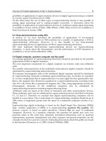
In section 3.1.1, the heat capacity and thermal conductivity of NbTi, YBCO, copper and
solder are given, we list the heat capacity C (J·kg
-1
·K
-1
·) and thermal conductivity k(W·m
-
1
·K
-1
) of other materials including Bi2223, stainless steel, silver.
i.
Bi2223
()
()
()
()
33
32 43
2223
32 63
4.5683 10 10
3.088 0.64996 8.23239 10 3.2406 10 10 40
58.32 3.18672 7.8786 10 6.5556 10 40 300
Bi

TTK
CT T T T KTK
TT TKTK
−
−−
−−

×≤


=− + + × + × ≤ ≤


−+ − × + × ≤≤


(33)
With mass density γ
Bi2223
=6500(kg·m
-3
).

Applications of High-Tc Superconductivity

88

()
()
()

()
34263
84
342 63
2223
84
42 63
0.02 55
0.474 8.43 10 3.25 10 6.595 10
55 77
2.81 10
0.195 9.424 10 3.4 10 6.237 10
77 113
2.673 10
4.749 0.102 9.901 10 4.167 10
Bi
TTK
TT T
KT K
T
kT
TT T
KT K
T
TT T
−− −
−
−− −
−
−−

≤

+× +× − ×

<≤

+×


=
+× +× −×

<<

+×

−+×−×
+
()
94
113 200
6.531 10
KT K
T
−














≤<


×


(34)
ii.
Silver

()
()
43 22
53 22
8.41 10 5.10 10 0.5566 1.6341 4 18
2.341 10 1.674 10 3.8384 50.775 (18 300 )
Ag
TTT KTK
CT
TTT KTK
−−
−−


×+×− + <≤

=

×−×+ − <≤


(35)
With mass density γ
Ag
=10490 (kg·m
-3
).

()
()
()
()
()
32
32
32
22
43.343 1227.2 10513 10254 4 10
0.6174 72.264 2816.5 37594 (10 38 )
0.0179 3.6865 253.64 6292.2 38 50
1.3 10 0.825 640.3 50 100
420 100 300
Ag

TTT KTK
TTT KTK
kT T T T KT K
TT KTK
KT K
−

×− + − <≤


−+ −+ <≤


=− + − + < ≤


−× − + <≤


<≤


(36)
iii.
Stainless steel (304L)

()
()
63 22
42

2 10 1.59 10 0.2644 0.4089 4 30
3.114 10 0.7171 1.7843 (30 300 )
ss
TTT KTK
CT
TT KTK
−−
−

×+×+ + <≤

=

×+ − <≤


(37)
With mass density γ
ss
=7900(kg·m
-3
).

() ( )
93 42
2.7041 10 3.3219 10 0.126 0.1877 4 300
ss
kT T T T KT K
−−
=× −× + − ≤≤ (38)

In this section, the longitudinal QPV and MQE are numerically simulated by solving Eq.(8)
in combination with Eqs. (10)-(12), (16), (25), (26) and (29)-(38) under adiabatic conditions.
Figs.12(a)-(c) show the temperature profiles at locations of 20 mm, 40 mm, 60 mm and 80
mm from the center with different external disturbances and transport currents. The
variations of n values with temperature are not considered in simulation. The hybrid
conductor was tested in magnetic field of 6 T which was applied for reducing its critical
current in measurement. The dependence of n values on temperature is very difficult to
obtain by experiment with supplying so high a transport current and background magnet.
Therefore, we used the constant n values in simulation. Usually, the n values will decrease
with increasing temperature, but we took n values approximately constant with fixed
magnetic field regardless of influence of temperature in order to simplify calculation. In
future, we should take NbTi and Bi2223 with small I
c
in experiment within magnet bore in
which temperature can be changed. Or the n values are measured by contact-free methods,
like those methods adopted in HTS at 77 K (Wang et al, 2004; Fukumoto et al, 2004).