Vibration Analysis and Control New Trends and Developments Part 9 ppt
Bạn đang xem bản rút gọn của tài liệu. Xem và tải ngay bản đầy đủ của tài liệu tại đây (2.97 MB, 25 trang )
Seismic Response Control Using Smart Materials
189
where W
D
is the energy loss per cycle and is the maximum cyclic displacement under
consideration. The secant stiffness (K
s
) is computed as
K
s
= (F
max
- F
min
) / (
max
-
min
) where F
max
and F
min
are the forces attained for the
maximum cyclic displacements
max
and
min
. The associated energy dissipation and the
equivalent viscous damping calculated are included in Table.1.
The effect of pre-strain is found at 2.5% pre strain applied in the form of deformation to the
sample, on two cyclic strains namely 4 % and 6 % (Fig.11.). An increase in the energy
dissipation can be observed as the cyclic strain amplitude increases. The energy dissipated
during cycling in pre-strained wires is considerably high compared to non-pre strained
wires as observed from the experiment. It is interested to observe that (Fig.13) leaving the
flat plateau; the response follows the elastic curve below 2% strain as obtained from the
quasi-static test. Hence the quasi- static behaviour gives the envelope curve for the cyclic
actions and a variety of hysteretic behaviour suitable for seismic devices can be obtained
with pre straining effect [Sreekala et al, 2010].
7. Modeling the maximum energy dissipation for the material under study
It is observed from the experiment that the wires pre strained to the middle of the strain
range gives the maximum energy dissipation(fig. 8). The behaviour can be predicted using
the following mathematical expressions.
{1/ }
n
E
Y
(2)
{1/ }
n
EYE
(3)
σ
*
denotes the stress in the pre strained wire at the beginning of the cycling. Here β can be
expressed as
.
in c
T
E f erf u
(4)
β denotes the one dimensional back stress, Y is the “yield” stress ,that is the beginning of the
stress- induced transition from austenite to martensite, n is the overstress power. In
equation (4) the unit step function activates the added term only during unloading
processes. In the descending curve it contributes to the back stress in a way that allows for
SMA stress-strain description. The term with (.) shows the ordinary time derivative.
y
y
E
EE
is a constant controlling the slope of σ – ε, where E is the elastic modulus of
austenite and E
y
is the slope after yielding.
Inelastic strain,
in
,is given by
in
E
(5)
Vibration Analysis and Control – New Trends and Developments
190
The error function, erf(x) ,and the unit step function, u(x) are defined as follows.
2
2
()
t
erf x e dt
(6)
() 1ux
, x ≥ 0 (7)
u(x) = 0 , x < 0 (8)
The basic expression obtained here for pre-strained wires is a modified form of the model
suggested by wilde et al, [12] which is used for predicting the tensile behaviour of SMA
materials. This mathematical expression describes the mechanical response of materials
showing hysteresis.
.
n
E
Y
(9)
where σ is the one dimensional stress and ε is the one-dimensional strain, β is the one
dimensional back stress , E elastic modulus , Y the yield stress and n the constant controlling
the sharpness of the transition from elastic to plastic states.
The modified Cozzarelli model suggested by Wilde et al represents the hardening of the
material after the transition from austenite to martensite is completed. Here in this case for
pre strained wires for maximum energy dissipation, the hardening branch has not been
considered which requires additional terms containing further unit step functions. The
model is rate and temperature independent. The requirement of zero residual strain at the
end of the loading process motivated the selection of the particular form of back stress
through the unit step function. The coefficients f
t
, and c are material constants controlling
the recovery of the elastic strain during unloading. Since the stress and strain were found to
be independent of the rate, the time differential can be eliminated. Hence equation (2) and
(3) can be used for predicting the behaviour after many cycles by appropriately changing
the values of ‘n’ and the starting stress value which follows the trend as in fig. 15. The
material constants for the wires tested were obtained as
f
t
= 0.115, C =0.001, n = 0.25, α = 0.055. Using Equations (2) and (3) the curves are
fitted. Fig. 15 gives the fitted curve for the maximum energy dissipation for the material
tested.
8. Various seismic response mitigation strategies
Earthquake engineering has witnessed significant development during the course of the last
two decades. Seismic isolation and energy dissipation are proved to be the most efficient
tools in the hands of design engineer in seismic areas to limit both relative displacements as
well as transmitted forces between adjacent structural elements to desired values. Parallel
development of new design strategies (the seismic software) and the perfection of suitable
mechanical devices to implement the strategies (the seismic hardware) made it possible to
achieve efficient seismic response control. An optimal combination of isolator and the
energy dissipater ensures complete protection of the structure during earthquake. Energy
dissipation and re-centering capability are the two important functions to cater this need.
Seismic Response Control Using Smart Materials
191
Most of the devices now in practice have poor re-centering capabilities. Instead of using a
single device a combination of devices can provide significant advantages
The chart shown below Fig.18 illustrates the various seismic response mitigation strategies.
0
200
400
600
800
1000
1200
0 0.02 0.04 0.06 0.08 0.1 0.12
strain
stress(N/mm2)
Experimental
Curve'"
Fitted Curve
Fig. 15. Cyclic behaviour of prestrained wires –maximum energy dissipation obtained and
the fitted curve.
Fig. 16. Various seismic response mitigation strategies
Vibration Analysis and Control – New Trends and Developments
192
Sl.no:
Nature of
Test
Pre- strain in
the wire
Cycling
Strain range
(%)
Average energy
dissipated per
cycle X10
-2
J
No: of
cycles
Equivalent
viscous
damping
1
Dynamic
Tests
Freq. of
operation
0.5 Hz.
(Sinusoidal
cyclic)
7%
6.5-7.5
6.0-8.0
5.0-9.0
4.0-10.0
3.0-11.0
1.3-12.0
00.30
00.60
06.70
18.60
33.00
-
10
10
a
10
a
10
a
10
a
-
0.02
0.02
0.06
0.07
0.09
-
2 6% 2-10
33.80
27.00
21.00
10
50
a
500
a
0.16
0.11
0.09
3 5%
4.5-5.5
4.0-6.0
3.0-7.0
00.50
04.60
07.70
10
10
a
10
a
0.04
0.13
0.12
4 4%
3.5-4.5
3.0-5.0
2.0-6.0
00.33
05.40
10.35
10
10
a
10
a
0.02
0.16
0.16
5 3%
2.5-3.5
2.0-4.0
01.01
01.91
10
10
a
0.05
0.04
6 2%
1.5-2.5
1.0-3.0
0.0-4.0
01.50
04.40
05.10
10
10
a
10
a
0.10
0.10
0.07
7 Nil
-3 - +3
-3 - +3
-4 - +4
07.30
06.40
05.10
25.
328
a
560
a
0.03
0.03
0.04
8 Nil
-3 - +3
-7 - +7
05.60
10.90
1500
140
a
0.03
0.045
Table 1. Evaluated parameters of the Nitinol wire.
a
- denotes
the number of cycles which are followed by the cumulative previous cycles.
From this diagram it is clear that for seismic mitigation, a combination of Seismic isolation
and Energy Dissipation is beneficial. Seismic Isolation can be implemented as explained
below:
- Through the reduction of the seismic response subsequent to the shift of the
fundamental period of the structure in an area of the spectrum poor in energy content
- Through the limitation of the forces transmitted to the base of the structure. A high
level of energy dissipation also characterizes this approach. So it represents a
combination of the two strategies of seismic mitigation. Isolation systems must be
capable of ensuring the following functions:
1. transmit vertical loads,
2. provide lateral flexibility,
3. provide restoring force,
4. provide significant energy dissipation.
Seismic Response Control Using Smart Materials
193
In each device, the constituent elements assume one or more of the four fundamental
functions listed above. Some of the cases hybrid systems prove to be very much beneficial.
For example, the strategy need to be adopted in suspension bridges is that of isolation and
energy dissipation as the vertical cables did not provide energy dissipation characteristics.
Hence dampers need to be provided and the hybrid system provide adequate protection
during seismic response. The Table 2 below provide various energy dissipators/dampers
along with their principle of operation
Classification Principles of operation
Hysteritic devices
Yielding of metals
Friction
Visco elastic devices
Deformation of visco elastic solids
Deformation of visco elastic fluids
Fluid orificing
Re centering Devices
Fluid pressurization and orificing
Friction spring action
Phase transformation of metals (Shape
memory alloys belong to this category)
Dynamic vibration absorbers
Tuned mass dampers
Tuned liquid dampers
Table 2.Various energy dissipation devices/damper
Fig. 17. Example of Composite Rubber/SMA spring damper
The unique constitutive behaviors of Shape Memory Alloys have attracted the attention of
researchers in the civil engineering community. The collective results of these studies
suggest that they can be used effectively for vibration control of structures through vibration
isolation and energy absorption mechanisms. Possible applications of SMA based devices
on Various structures for vibration control is shown in Fig.18,
For the analysis of structures, an equivalent Single Degree Of Freedom (SDOF) system can
be utilized. The following mechanical model can represent the behavior of the energy
dissipating system (Fig.19a). If re centering device is utilized the hysterisis should be
adequately represented using mathematical models.
Vibration Analysis and Control – New Trends and Developments
194
(i)
(ii)
(iii)
Fig. 18. Possible Applications of the Devices (i) Restrainers in Bridges (ii) Diagonal braces in
buildings (iii) Cable stays (iv) combination of isolators and dampers in bridges
a) b)
Fig. 19. a) Equivalent mechanical model of the SDOF scaled structure
b) The hysterisis /energy dissipation behavior of the re-centering device
Seismic Response Control Using Smart Materials
195
9. Conclusion
There have been considerable research efforts in seismic response control for the past
several decades. Due to the distinctive macroscopic behaviour like super elasticity, Shape
Memory Alloys are the basis for innovative applications such as devices for protecting
buildings from structural vibrations. Super elastic properties of Nitinol wires have been
established from the experiments conducted and the salient features to be highlighted from
the study are
The material’s application can be made suitable for seismic devices like recentering,
supplementally recentering or in the case of non-recentering devices, as a variety of
hysteretic behaviors were obtained from the tests.
Cyclic behavior of the non pre strained wires especially energy dissipation capability,
equivalent viscous damping and secant stiffness are not very sensitive to the number of
cycles in the frequency range of interest (0.5- 3Hz.) as observed from constant
amplitude loading.
Pre-strained super elastic wires shows higher energy dissipation capability and
equivalent damping when cycled around the midpoint of the strain range obtained
from quasi-static curve. It is found from the experiment that the pre strain value of 6 %,
with amplitude cycles which covers 2-10% gives higher energy dissipation.
For possible application of vibration control devices in structural systems, a judicious
selection of the wire under tension mode can be selected between pre strained and non-
pre strained wires. However application of pre strained wires in the system provides
excellent energy dissipation characteristics but it requires skilled and sophisticated
mechanism to maintain/provide the required pre strain.
The mathematical model predicts the maximum energy dissipation capability of the
material namely pre strained nitinol wires under study.
The test results shows immense promise on SMA based devices which can be used for
vibration control of variety of structures(New designs and restoration of structures).
SMA structural elements/devices can be located at key locations of the structure to
reduce the seismic vibrations.
10. Acknowledgment
The paper has been published with the kind approval of Director, CSIR-Structural
Engineering Research Centre, Chennai. The constant encouragement, and support provided
by the Director General-CSIR, Dr. Sameer K Brahmachari is gratefully acknowledged. The
help and support provided by all colleagues of Advanced Seismic Testing and Research
Laboratory in carrying out the experimental work deserve acknowledgement.
11. References
Birman, V (1997) Review of Mechanics of Shape Memory Alloy Structures Applied Mechanics
Review 50 629-645
Birman, V (1997) Effect of SMA dampers on nonlinear vibrations of elastic structures
Proceedings of SPIE 3038 ,268-76
Vibration Analysis and Control – New Trends and Developments
196
Clark, P W; Aiken, I D; Kelly, J M; Higashino, M and Krumme, R C(1996) Experimental
and analytical studies of shape memory alloy damper for structural control Proc.
Passive damping (San Diego,CA 1996)
Cardone D, Dolce M, Bixio A and Nigro D 1999 Experimental tests on SMA elements
MANSIDE Project (Rome, 1999) (Italian Department for National Technical Services)
II85-104 Da GZ, Wang TM, Liu Y, Wamg CM( 2001) Surgical treatment of tibial and
femoral fractures with TiNi Shape memory alloy interlocking intra medullary nails
The international conference on Shape Memory and Superelastic Technologies and Shape
Memory materials, Kunming, China
Dolce M (1994) Passive Control of Structures Proceedings of the 10
th
European Conference
on Earthquake Engineering, Vienna, 1994.
Duerig, T; Tolomeo, D and Wholey, M. (2000), An overview of superelastic stent design
Minimally Invasive Therapy & Allied Technologies. , 2000:9(3/4) 235–246.
Eaton, J P. (1999) Feasibility study of using passive SMA absorbers to minimize secondary
system structural response , Master Thesis ,Worcester polytechnic Institute, M A
Humbeeck, JV (2001) Shape Memory Alloys: a material and a technology Advanced
Engieering Materials 3 837-850
Miyazaki, S; Imai, T; Igo, Y. And Otsuka, K(1986b), Effect of cyclic deformation on the
pseudoelasticity characteristics of Ti–Ni alloys. Metall. Trans. A. 17115–120.
Pelton, A; DiCello,J; and Miyazaki,S. , (2000), Optimisation of processing and properties of
medical grade nitinol wire. Minimally Invasive Therapy & Allied Technologies. ,
2000:9(1) 107–118.
Sreekala, R; Avinash, S; Gopalakrishnan, N; and Muthumani, K(2004) Energy Dissipation and
Pseudo Elasticity in NiTi Alloy Wires SERC Research Report MLP 9641/19, October 2004
Sreekala, R; Avinash, S; Gopalakrishnan, N; Sathishkumar, K and Muthumani, K(2005)
Experimental Study on a Passive Energy Dissipation Device using Shape Memory
Alloy Wires, SERC Research Report MLP 9641/21, April 2005
Sreekala,. R;. Muthumani, K; Lakshmanan, N; Gopalakrishnan, N & Sathishkumar, K
(2008),. Orthodontic arch wires for seismic risk reduction, Current Science,
ISSN:0011-3891, Vol. 95, No:11, pp 1593-1599.
Sreekala,. R,;. Muthumani,. K(2009),. Structural Application of Smart materials,. In:. Smart
Materials,. Edited by Mel Shwartz, . CRC press, Taylor & Francis Group,. pp. 4-1 to
4-7,. Taylor &Francis Publications,. ISBN-13:978-1-4200-4372-3,. Boca raton, FL,USA
Sreekala,. R;. Muthumani, K; Lakshmanan, N; Gopalakrishnan, N; Sathishkumar, K; Reddy, G,R
& Parulekar Y M. (2010),. A Study on the suitability of NiTi wires for Passive Seismic
Response Control Journal of Advanced Materials, ISSN 1070-9789, Vol. 42, No:2,pp. 65-76.
Stöckel,D. and Melzer, A. ,, Materials in Clinical Applications. , ed. P. Vincentini Techna Srl.
,1995, 791–98.
Wilde, K; Gardoni, P. , and Fujino Y. ,(2000) Base isolation system with shape memory alloy
device for elevated highway bridges Engineering Structures 22 222-229.
10
Whys and Wherefores of Transmissibility
N. M. M. Maia
1
, A. P. V. Urgueira
2
and R. A. B. Almeida
2
1
IDMEC-Instituto Superior Técnico, Technical University of Lisbon
2
Faculdade de Ciências e Tecnologia, Universidade Nova de Lisboa
Portugal
1. Introduction
The present chapter draws a general overview on the concept of transmissibility and on its
potentialities, virtues, limitations and possible applications. The notion of transmissibility
has, for a long time, been limited to the single degree-of-freedom (SDOF) system; it is only
in the last ten years that the concept has evolved in a consistent manner to a generalized
definition applicable to a multiple degree-of-freedom (MDOF) system. Such a generalization
can be and has been not only developed in terms of a relation between two sets of harmonic
responses for a given loading, but also between applied harmonic forces and corresponding
reactions. Extensions to comply with random motions and random forces have also been
achieved. From the establishment of the various formulations it was possible to deduce and
understand several important properties, which allow for diverse applications that have
been envisaged, such as evaluation of unmeasured frequency response functions (FRFs),
estimation of reaction forces and detection of damage in a structure. All these aspects are
reviewed and described in a logical sequence along this chapter.
The notion of transmissibility is presented in every classic textbook on vibrations, associated
to the single degree-of-freedom system, when its basis is moving harmonically; it is defined
as the ratio between the modulus of the response amplitude and the modulus of the
imposed amplitude of motion. Its study enhances some interesting aspects, namely the fact
that beyond a certain imposed frequency there is an attenuation in the response amplitude,
compared to the input one, i.e., one enters into an isolated region of the spectrum. This
enables the design of modifications on the dynamic properties so that the system becomes
“more isolated” than before, as its transmissibility has decreased.
Usually, the transmissibility of forces, defined as the ratio between the modulus of the
transmitted force magnitude to the ground and the modulus of the imposed force
magnitude, is also deduced and the conclusion is that the mathematical formula of the
transmissibility of forces is exactly the same as for the transmissibility of displacements. As
it will be explained, this is not the case for multiple degree of freedom systems.
The question that arises is how to extend the idea of transmissibility to a system with N
degrees-of-freedom, i.e., how to relate a set of unknown responses to another set of known
responses, for a given set of applied forces, or how to evaluate a set of reaction forces from a
set of applied ones. Some initial attempts were given by Vakakis et al. (Paipetis & Vakakis,
1985; Vakakis, 1985; Vakakis & Paipetis, 1985; 1986), although that generalization was still
Vibration Analysis and Control – New Trends and Developments
198
limited to a very particular type of N degree-of-freedom system, one where a set constituted
by a mass, stiffness and damper is repeated several times in the vertical direction. The works
of (Liu & Ewins, 1998), (Liu, 2000) and (Varoto & McConnell, 1998) also extend the initial
concept to N degrees-of-freedom systems, but again in a limited way, the former using a
definition that makes the calculations dependent on the path taken between the considered
co-ordinates involved, the latter by making the set of co-ordinates where the displacements
are known coincident to the set of applied forces.
An application where the transmissibility seems of great interest is when in field service one
cannot measure the response at some co-ordinates of the structure. If the transmissibility
could be evaluated in the laboratory or theoretically (numerically) beforehand, then by
measuring in service some responses one would be able to estimate the responses at the
inaccessible co-ordinates.
To the best knowledge of the authors, the first time that a general answer to the problem has
been given was in 1998, by (Ribeiro, 1998). Surprisingly enough, as the solution is very
simple indeed. In what follows, a chronological description of the evolution of the studies
on this subject is presented.
2. Transmissibility of motion
In this section and next sub-sections the main definitions, properties and applications will be
presented.
2.1 Fundamental formulation
The fundamental deduction (Ribeiro, 1998), based on harmonically applied forces (easy to
generalize to periodic ones), begins with the relationships between responses and forces in
terms of receptance: if one has a vector
F
A
of magnitudes of the applied forces at co-
ordinates A, a vector
U
X
of unknown response amplitudes at co-ordinates U and a vector
X
K
of known response amplitudes at co-ordinates K, as shown in Fig. 1.
Fig. 1. System with co-ordinates A, U, K
One may establish the following relationships:
UUAA
=
X
HF (1)
Whys and Wherefores of Transmissibility
199
KKAA
=
X
HF (2)
where
H
UA
and
H
KA
are the receptance frequency response matrices relating co-ordinates
U and A, and K and A, respectively. Eliminating
F
A
between (1) and (2), it follows that
UUAKAK
+
=
X
HHX
(3)
or
UK
=
X
TX
(A)
UK
(4)
where
+
H
KA
is the pseudo-inverse of
H
KA
. Thus, the transmissibility matrix is defined as:
UA KA
+
=THH
(A)
UK
(5)
Note that the set of co-ordinates where the forces are (or may be) applied (A) need not
coincide with the set of known responses (K). The only restriction is that – for the pseudo-
inverse to exist – the number of K co-ordinates must be greater or equal than the number of
A co-ordinates.
An important property of the transmissibility matrix is that it does not depend on the
magnitude of the forces, one simply has to know or to choose the co-ordinates where the
forces are going to be applied (or not, as one can even choose more co-ordinates A if one is
not sure whether or not there will be some forces there and, later on, one states that those
forces are zero) and measure the necessary frequency-response-functions.
2.2 Alternative formulation
An alternative approach, developed by (Ribeiro et al., 2005) evaluates the transmissibility
matrix from the dynamic stiffness matrices, where the spatial properties (mass, stiffness,
etc.) are explicitly included.
The dynamic behaviour of an MDOF system can be described in the frequency domain by
the following equation (assuming harmonic loading):
=
Z
XF
(6)
where
Z
represents the dynamic stiffness matrix,
X
is the vector of the amplitudes of the
dynamic responses and
F
represents the vector of the amplitudes of the dynamic loads
applied to the system.
From the set of dynamic responses, as defined before, it is possible to distinguish between
two subsets of co-ordinates K and U; from the set of dynamic loads it is also possible to
distinguish between two subsets, A and B, where A is the subset where dynamic loads may
be applied and B is the set formed of the remaining co-ordinates, where dynamic loads are
never applied. One can write
X
and
F
as:
,
KA
UB
⎧
⎫⎧⎫
==
⎨
⎬⎨⎬
⎩⎭ ⎩⎭
XF
XF
X
F
(7)
With these subsets, Eq. (6) can be partitioned accordingly:
Vibration Analysis and Control – New Trends and Developments
200
A
KAU K A
BK BU U B
⎡
⎤⎧ ⎫ ⎧ ⎫
=
⎨
⎬⎨ ⎬
⎢⎥
⎣
⎦⎩ ⎭ ⎩ ⎭
Z
ZXF
Z
ZXF
(8)
Taking into account that co-ordinates B represent the ones where the dynamic loads are
never applied, and considering that the number of these co-ordinates is greater or equal to
the number of co-ordinates U, from Eq. (8) it is possible to obtain the unknown response
vector:
, # #
B
UBUBKK
BU=≥
⇓
=−
+
F0
X
ZZX
(9)
where
BU
+
Z
is the pseudo-inverse of
B
U
Z
. Therefore, this means that the transmissibility
matrix can also be defined as
(A)
UK
=−
BU BK
+
TZZ
(10)
Eq. (10) is an alternative definition of transmissibility, based on the dynamic stiffness
matrices of the structure. Therefore,
(A)
UK
+
==−
UA KA BU BK
+
THH ZZ
(11)
Taking into account that the dynamic stiffness matrix for an undamped system is described
in terms of the stiffness and mass matrices,
2
ω
=−ZK M
, one can now relate the
transmissibility functions to the spatial properties of the system. To make this possible, one
must bear in mind that it is mandatory that both conditions regarding the number of co-
ordinates be valid, i. e.,
## # #andBU K A≥≥ (12)
2.3 Numerical example
An MDOF mass-spring system, presented in Fig. 2, will be used to illustrate the principal
differences observed between the transmissibilities and FRFs curves. This is a six mass-
spring system (designated as original system), possessing the characteristics described in
Table 1.
The subsets of known and unknown responses are assumed as:
{}
246
T
T
K
XXX=X and
{}
135
T
T
U
XXX=X (13)
The number of loads can be grouped in the sub-set
A
F
(even if some of them are, in certain
cases, null) and in subset
B
F
.
{}
456
T
T
A
FFF=F and
{}
123
T
T
B
FFF=F (14)
According to Eq. (11), and considering the above-defined subsets, the transmissibility matrix
is given by:
Whys and Wherefores of Transmissibility
201
Original System
kg
N/m
m
1
m
2
m
3
m
4
m
5
m
6
k
1
k
2
k
3
k
4
k
5
k
6
k
7
k
8
k
9
k
10
k
11
7
7
4
3
6
8
10
5
10
5
4.0x10
5
5.0x10
5
7.0x10
5
2.0x10
5
8.0x10
5
3.0x10
5
6.0x10
5
3.0x10
5
5.0x10
5
Table 1. Characteristics of the original system
Fig. 2. Mass-spring MDOF system
Vibration Analysis and Control – New Trends and Developments
202
12 14 16
14 15 16 24 25 26
34 35 36 44 45 46
32 34 36
54 55 56 64 65 66
52 54 56
11 13 15
21 23 25
31 33 3
TTT
HHHHHH
TTT HHHHHH
HHHHHH
TTT
ZZZ
ZZZ
ZZZ
+
⎡⎤
⎡
⎤⎡ ⎤
⎢⎥
⎢
⎥⎢ ⎥
=
⎢⎥
⎢
⎥⎢ ⎥
⎢⎥
⎢
⎥⎢ ⎥
⎣
⎦⎣ ⎦
⎢⎥
⎣⎦
=−
(A) (A) (A)
(A) (A) (A)
(A) (A) (A)
12 14 16
22 24 26
5323436
ZZZ
ZZZ
ZZZ
⎡
⎤⎡ ⎤
⎢
⎥⎢ ⎥
⎢
⎥⎢ ⎥
⎢
⎥⎢ ⎥
⎣
⎦⎣ ⎦
+
(15)
The characteristics of the system of Fig. 2 are presented in Table 1.
It may be noted from Fig. 3 that the maxima of the transmissibility curves occur all at the same
frequencies. It can also be observed that the maxima and minima of the transmissibility curves
do not coincide with the maxima and minima of the FRF curves. No simple relationships (if
any) can be established between the picks and anti-picks of the transmissibilities and FRFs.
Transmissibilities have a local nature and therefore they do not reflect the existence of the
global properties of the system (natural frequencies and damping ratios).
0 20 40 60 80 100 120 140 160 180 200
Frequency [Hz]
-280
-240
-200
-160
-120
-80
-40
0
40
80
120
Magnitude [dB]
T
14
(Orig.)
T
52
(Orig.)
T
56
(Orig.)
H
14
(Orig.)
H
35
(Orig.)
Fig. 3. Some transmissibilities and FRFs curves of the original system
2.4 Transmissibility properties
The formulation presented in section 2.1 allows us to extract some important properties for
the transmissibility matrix
T
(A)
UK
. From Eq. (3) and (5) it is possible to conclude that the
transmissibility matrix is independent from the force vector
A
F
(Note that
A
F
is eliminated
between eqs. (1) and (2)). This means that any change verified in one of the force values,
acting along with co-ordinates of set A, will not affect
T
(A)
UK
. This change can be due, for
instance, to the alteration of mass values associated to co-ordinates A or stiffness values of
springs interconnecting those co-ordinates.
Additionally, to highlight that characteristic of matrix
T
(A)
UK
, it can be verified from Eq. (10)
that there is no part of matrix
Z involving co-ordinates of set A (neither
A
K
Z
nor
A
U
Z
). This
statement reinforces the previous conclusion extracted from Eq. (5) and will lead to the
formulation of two properties, as follows:
Whys and Wherefores of Transmissibility
203
Property 1.
The transmissibility matrix does not change if some modification is made on the mass
values of the system where the loads can be applied – subset A.
Property 2. The transmissibility matrix does not change if some modification is made on the stiffness
values of springs interconnecting co-ordinates of subset A – (where the loads can be applied).
In fact, any changes in the mass values associated to co-ordinates A and/or any changes in
the stiffness values of springs interconnecting co-ordinates A, will affect the inertia forces
and elastic forces, respectively, acting along those co-ordinates and thus belonging to
A
F
.
The same MDOF system presented in Fig. 2 will be used to illustrate the transmissibility
properties. In Table 2 four different modifications are made in the original system.
Situations I and II correspond to modifications on the original masses; situations III and IV
correspond to modifications on stiffness. Situations I and III only involve co-ordinates A,
whereas situations II and IV involve co-ordinates pertaining to both sets A and B.
Choosing, for instance, the transmissibility function
()
52
A
T , one obtains the results presented
in Figs. 4 and 5, where one can see that
()
52
A
T and
()
14
A
T
remain the same only when changes
are made at co-ordinates A, where the forces are applied.
2.5 Evaluation of the transmissibility from measurement responses
In 1999, (Ribeiro et al., 1999) and (Maia et al., 1999) showed how the transmissibility matrix
could be evaluated directly from the measurement of the responses, rather than measuring
the frequency response functions. In Eq. (4), the problem is to evaluate the
UK× values of
T
(A)
UK
knowing
X
U
and
K
X
. This can be achieved by applying various sets of forces, at a
time, on co-ordinates
A. Let
(1)
A
F
be the first set of applied forces (amplitudes). Then,
=
X
TX
(1) (A) (1)
UUKK
(16)
Original System Situation I Situation II Situation III Situation IV
kg
N/m
m
1
m
2
m
3
m
4
m
5
m
6
k
1
k
2
k
3
k
4
k
5
k
6
k
7
k
8
k
9
k
10
k
11
7
7
4
3
6
8
10
5
10
5
4.0x10
5
5.0x10
5
7.0x10
5
2.0x10
5
8.0x10
5
3.0x10
5
6.0x10
5
3.0x10
5
5.0x10
5
13
12
14
13
14
13
9.0x10
5
9.0x10
6
10.0x10
5
unchanged value
Table 2. Characteristics of the modifications made in the original system
Vibration Analysis and Control – New Trends and Developments
204
0 20406080100120140160180200
Frequency [Hz]
-80
-60
-40
-20
0
20
40
60
80
100
Transmissibility [dB]
T
52
(orig.)
T
52
(Sit. I)
T
52
(Sit. II)
Fig. 4. Transmissibility
()
52
A
T
, for the original system and the modified systems I e II
0 20 40 60 80 100 120 140 160 180 200
Frequency [Hz]
-100
-80
-60
-40
-20
0
20
40
60
80
Transmissibility [dB]
T
14
(orig.)
T
14
(Sit. III)
T
14
(Sit. IV)
Fig. 5. Transmissibility
()
14
A
T
, for the original system and the modified systems III e IV
However, when forces change, the transmissibility matrix does not, although the responses
themselves do. Therefore, if another test is performed, with a set of forces
linearly
independent
of the first one – though applied at the same co-ordinates –
(2)
A
F
, a new set of U
equations can be obtained, which are linearly independent of the first ones. If
K tests are
undertaken on the structure, with linearly independent forces always applied at the
A set of
co-ordinates, one can obtain a system of
UK
×
equations to solve for the same number of
(A)
UK
T
unknowns:
⎡
⎤⎡ ⎤
=
⎣
⎦⎣ ⎦
""XX X TXX X
(1) (2) (K) (A) (1) (2) (K)
UU U UKKK K
(17)
From which
1
−
⎡
⎤⎡ ⎤
=
⎣
⎦⎣ ⎦
""TXX XXX X
(A) (1) (2) (K) (1) (2) (K)
UK U U U K K K
(18)
Whys and Wherefores of Transmissibility
205
Note: an easy way to obtain the K sets of linearly independent forces is to apply a single
force at each of the
A locations at a time.
2.6 The distributed forces case
In (Ribeiro, Maia, & Silva, 2000b) the authors discussed the transmissibility between the two
sets of co-ordinates
U and K when a distributed force is applied to the structure. Such a force
should be discretized to form the
A set of applied forces. The issue was then to study what
happened if one only took a subset of those co-ordinates
A, which implies the reduction or
condensation of the applied forces to such a subset and to ask the question: “how to study
the transmissibility of responses from a set of condensed forces?”. Let the set
A be composed
by the set
C to where one wishes to condense the forces and the set D of the remaining co-
ordinates, so that:
⎧
⎫
=
⎨
⎬
⎩⎭
F
F
F
C
A
D
(19)
If one wishes to condense
F
A
to
F
C
, one needs to assume some relationship between F
D
and
F
C
, i.e, one cannot contemplate the case where all the applied forces are completely
independent from each other. However, this is not a big restriction, as it seems reasonable to
expect that the applied forces exhibit a more or less fixed spatial pattern along the structure.
Therefore, let us assume a linear relationship between the sets of forces
F
D
and F
C
,
through the matrix
P
D
C
:
=
F
PF
DDCC
(20)
If matrices
UA
H
and
K
A
H
from eqs. (1) and (2) are partitioned into
[
]
UA UC UD
= #HH H
(21)
[
]
KA KC KD
=
#HH H
(22)
and one has Eq. (19) into account, then eqs. (1) and (2) become
UUC UD
=+
X
HF HF
CD
(23)
KKC KD
=+
X
HF HF
CD
(24)
Substituting Eq. (20) in eqs. (23) and (24) and eliminating
C
F
, it follows that
()()
UUCUD KCKD K
+
=+ +
X
HHPHHPX
DC DC
(25)
Therefore, one has now, instead of Eq. (4), another one relating
U
X
and
K
X
, through a new
transmissibility matrix referred to the new subset of co-ordinates
C:
UK
=
X
TX
(C)
UK
(26)
Vibration Analysis and Control – New Trends and Developments
206
where
()()
UC UD KC KD
+
=+ +THHPHHP
(C)
UK DC DC
(27)
Note: for the pseudo-inverse to exist, the number of
K co-ordinates must be higher than the
number of
C co-ordinates. This is obviously verified, as
##KA≥
and # #AC> . It should
also be stressed that although referred to a reduced set of co-ordinates
C where the forces
are applied, the transmissibility matrix still relates the responses
U and K and so it keeps the
same size.
In (Ribeiro, Maia, & Silva, 2000a), (Ribeiro, Maia, & Silva, 2000b) and (Maia et al., 2001) the
authors summarize some of the previous works and suggest some other possible
applications for the transmissibility concept, namely in the area of damage detection. In this
area, there has been some activity trying to use the transmissibility as defined, as well as
some other variations of it, with limited results in [(Sampaio et al., 1999; 2000; 2001)], but
with some promising evolution in [(Maia et al., 2007)].
An example is presented in order to illustrate the above discussion: a cantilevered beam is
subjected to the loading shown in Fig. 6.
Fig. 6. Example of a loaded beam
It is assumed that forces are applied at co-ordinates 1 to 6 but the forces at co-ordinates 2 to
5 can be related to those applied at 1 and 6 through the expression:
2
31
46
5
41
32
1
23
5
14
f
f
f
f
f
f
⎧⎫ ⎡ ⎤
⎪⎪ ⎢ ⎥
⎧
⎫
⎪⎪
⎢⎥
=⇒=
⎨
⎬⎨⎬
⎢⎥
⎩⎭
⎪⎪
⎢⎥
⎪⎪
⎩⎭ ⎣ ⎦
FPF
DDCC
(28)
One can further assume that the responses at co-ordinates 1 and 2 can be measured and
those at co-ordinates 4 and 5 can be computed through the transmissibility, i.e.,
UK
=
X
TX
(C)
UK
, with
4
5
U
⎧
⎫
=
⎨
⎬
⎩⎭
X
X
X
,
1
2
K
⎧
⎫
=
⎨
⎬
⎩⎭
X
X
X
and
Whys and Wherefores of Transmissibility
207
()()
41 46 42 43 44 45 11 16
51 56 52 53 54 55 21 26
41
32
1
23
5
14
UC UD KC KD
HH HHHH HH
HH HHHH HH
+
=+ + ⇒
⎛⎞⎛
⎡⎤
⎜⎟⎜
⎢⎥
⎡
⎤⎡ ⎤ ⎡ ⎤
⎜⎟⎜
⎢⎥
=+
⎢
⎥⎢ ⎥ ⎢ ⎥
⎜⎟⎜
⎢⎥
⎣
⎦⎣ ⎦ ⎣ ⎦
⎜⎟⎜
⎢⎥
⎜⎟⎜
⎣⎦
⎝⎠⎝
THHPHHP
T
(C)
UK DC DC
(C)
UK
12 13 14 15
22 23 24 25
41
32
1
23
5
14
HHHH
HHHH
+
⎞
⎡
⎤
⎟
⎢
⎥
⎡⎤
⎟
⎢
⎥
+
⎢⎥
⎟
⎢
⎥
⎣⎦
⎟
⎢
⎥
⎟
⎣
⎦
⎠
(29)
2.7 The random forces case
Often one has to deal with random forces, for instance when a structure is submitted to
environmental loads. The cases that have been addressed so far were limited to harmonic or
periodic forces. The generalization to random forces has been derived in [(Ribeiro et al.,
2002; Fontul et al., 2004)], now in terms of power spectral densities, rather than in terms of
response amplitudes. Let
KK
S
denote the auto-spectral density of the responses
K
X
and
KU
S
the cross-spectral density between responses
K
X
and
U
X
. Then, it can be shown (see
[(Fontul, 2005)] for specific details) that both are related through the same transmissibility
matrix as before (using Eq. (5), for instance):
TT
KU KK
=
S
TS
(A)
UK
(30)
2.8 Some possible applications
2.8.1 Transmissibility of motion in structural coupling
This topic has been addressed in (Devriendt, 2004; Ribeiro et al., 2004; Devriendt & Fontul,
2005). Let us consider a main structure, to which an additional structure is coupled though
some coupling co-ordinates, i.e., the additional structure applies a set of forces (and moments)
to the main structure. As the transmissibility between two sets of responses on the main
structure does not depend on the magnitude of those forces, the transmissibility matrix of the
main structure is equal to the transmissibility matrix of the total structure (main + additional).
In other words, under certain conditions, the transmissibility matrix of the main structure
remains unchanged, even if an additional structure is coupled to the main one. To make this
property valid it is necessary to consider a sufficient number of coupled co-ordinates.
Although it might be argued that a reduced number of coupling co-ordinates would hamper
the results since it would not include information about some modes, it has been shown in
(Devriendt, 2004; Ribeiro et al., 2004; Devriendt & Fontul, 2005) that, as long as there is enough
information regarding the modes included in the frequency range of interest the minimum
number of coupling co-ordinates can be reduced without deterioration of the results.
2.8.2 Evaluation of unmeasured frequency response functions
Recent papers [(Maia et al., 2008; Urgueira et al., 2008)] have explored some invariance
properties of the transmissibility, namely when modifications are made in terms of masses
Vibration Analysis and Control – New Trends and Developments
208
and/or stiffnesses at the co-ordinates where the forces are applied, to be able to estimate the
new FRFs in locations that become no longer accessible. For instance, if one calculates the
transmissibility matrix at some stage between two sets of responses for a given set of
applied forces and later on there are some modifications at the force co-ordinates due to
some added masses, the FRFs will change but the transmissibility remains the same. This
allows the estimation of the new FRFs. So, initially one has
(1) (1) (1) (1)
+
=
UUAKAK
XHHX and
later on one has
(2) (2) (2) (2)
UUAKAK
+
=XHHX. As the transmissibility remains unchanged, one
has
(1) (1) (2) (2)
UA KA UA KA
+
+
==THH H H
(A)
UK
(31)
and one can calculate, for instance,
(2)
UA
H
, given by:
(2) (2)
UA KA
=HTH
(A)
UK
(32)
2.9 Direct transmissibility
From the definition given before one has,
UUAKAK K
+
==
X
HHX TX
(A)
UK
(33)
which, as explained, is a generalisation from the one degree of freedom system. However, in
some cases it might be useful to divide two responses directly. In strict sense that is a
transmissibility only if a single force is applied. Otherwise, one has to name it differently,
like pseudo-transmissibility (e.g. (Sampaio et al., 1999)), scalar transmissibility (Devriendt et
al., 2010) or direct transmissibility, which is the one we shall adopt.
Direct transmissibilities will depend on the force magnitudes (as well as location, of course).
For example, dividing Eq. (33) by one of the amplitudes
K
X
, say
s
X , one has:
or
Us Ks Us Ks
XX==TT
(A) (A)
UK UK
XX
τ
τ
(34)
It is easier to understand the implications of both definitions through an example: let
U
X
,
K
X
, and
A
F
be given respectively by
135
246
UKA
XXF
XXF
⎧
⎫⎧⎫⎧⎫
===
⎨
⎬⎨⎬⎨⎬
⎩⎭ ⎩⎭ ⎩⎭
XXF (35)
The relation between
U
X
and
K
X
would be:
113143 1133144
223344 2233244
XTTX XTXTX
XTTX XTXTX
=+
⎧⎫⎡ ⎤⎧⎫
=⇒
⎨⎬ ⎨⎬
⎢⎥
=+
⎩⎭⎣ ⎦⎩⎭
(36)
Dividing Eq. (36) by, say,
3
X , it follows that
or
1 3 13 14 4 3 13 13 14 43
2 3 23 24 4 3 23 23 24 43
XX T TXX T T
XX T TXX T T
τ
τ
τ
τ
=+ =+
=+ =+
(37)
Whys and Wherefores of Transmissibility
209
One can also write:
1155166
15 5 16 6
1
13
3355366
3355366
XHFHF
HF HF
X
XHFHF
XHFHF
τ
=+
⎧
+
⇒==
⎨
=+
+
⎩
(38)
From Eq. (38) it is clear that the direct transmissibility
13
τ
depends on the magnitudes of
5
F
and
6
F
, unless the relation
56
FF
remains constant. Only in the case where there is just a
single force one has a coincidence between both types of transmissibility.
Both kinds of definitions can be useful. For instance, concerning now the direct
transmissibilities, one can see that from Eq. (37) one can calculate
13
τ
and
23
τ
from
43
τ
, and
one can eliminate
43
τ
between both equations and establish a relationship between
13
τ
and
23
τ
, therefore allowing the evaluation of one of them from the other. Moreover and similarly
to what was mentioned in section 2.5, the direct transmissibilities allow the calculation of
the other ones.
To illustrate the main differences between the curves of general and the direct
transmissibilities, the MDOF system presented in Fig. 2 has been used. In Fig. 7 some direct
transmissibility curves are presented.
0 20 40 60 80 100 120 140 160 180 200
Frequency [Hz]
-80
-60
-40
-20
0
20
40
60
80
Direct Trans. [dB]
τ
23
(Orig.)
τ
45
(Orig.)
τ
56
(Orig.)
Fig. 7. Some direct transmissibility curves from the system of Fig. 2
By comparing the results of the transmissibilities of Fig. 3 with the curves obtained with the
direct transmissibilities, Fig. 7, one can see that both look like FRFs, though it may be noted
that in the case of the transmissibilities all the maxima occur at the same frequencies; the
same is not true with the direct transmissibilities, where each curve presents distinct
maxima.
2.10 Other applications
Other works have presented the possibility of using the transmissibility concept for model
updating (Steenackers et al., 2007) and to identify the dynamic properties of a structure
(Devriendt & Guillaume, 2007; Devriendt, De Sitter, et al., 2009; Devriendt et al., 2010).
Vibration Analysis and Control – New Trends and Developments
210
Other recent studies have applied the transmissibility to the problem of transfer path
analysis in vibro-acoustics (Tcherniak & Schuhmacher, 2009) and for damage detection
(Canales et al., 2009; Devriendt, Vanbrabant, et al., 2009; Urgueira et al., 2011).
3. Transmissibility of forces
3.1 In terms of frequency response functions
Another important topic may be the prediction of the dynamic forces transmitted to the
ground when a machine is working. For a single degree of freedom, the solution is well
known and the transmissibility is defined as the ratio between the transmitted load (the
ground reaction) and the applied one, for harmonic excitation. For an MDOF system, one
has to relate the known applied loads (
K
F
) to the unknown reactions (
U
F
), Fig. 8.
The displacements at the co-ordinates of one set (the set of the reactions) are constrained, so
they must also be known (possibly zero).
The inverse problem may also be of interest, i.e., to estimate the loads applied to a structure
(wind, traffic, earthquakes, etc.) from the measured reaction loads. Once the load
transmissibility matrix is established between the appropriate sets, the measurement of the
reactions is expected to allow for the estimation of the external loads.
1
K
F
2
K
F
3
K
F
[
]
[
]
[
]
,,
M
KC
1
K
F
2
K
F
3
K
F
[
]
[
]
[
]
,,
M
KC
⇒
1
U
F
2
U
F
3
U
F
Fig. 8. Structure with applied loads and reactions in dynamic equilibrium
This topic has been addressed in (Maia et al., 2006); the force transmissibility may also be
defined either in terms of FRFs or in terms of dynamic stiffnesses. Let
K
X
and
U
X
be the
responses corresponding to
K
F
and
U
F
, respectively, and
C
X
the responses at the
remaining co-ordinates; then,
KKKKU
K
UUKUU
U
CCKCU
⎧⎫⎡ ⎤
⎧
⎫
⎪⎪
⎢⎥
=
⎨
⎬⎨⎬
⎢⎥
⎩⎭
⎪⎪
⎢⎥
⎩⎭⎣ ⎦
X
F
X
F
X
ΗΗ
ΗΗ
ΗΗ
(39)
Assuming the responses at the reactions co-ordinates as zero, i.e.,
U
=
X
0 , it follows that:
1
UUKK
UU
−
=−
F
F
ΗΗ
(40)
Whys and Wherefores of Transmissibility
211
Therefore, the force transmissibility is defined as:
1
UK UK
UU
−
=−T
ΗΗ
(41)
If the displacements at the co-ordinates of the reactions are not zero, or in the more general
case when the two sets of loads are not the applied loads and the reactions, but any disjoint
sets that encompass all the loads applied to the structure, it is easy to show (Maia et al.,
2006) that:
1
UUKK U
UU
−
=+
F
FX
ΤΗ
(42)
3.2 In terms of dynamic stiffness
Instead of Eq. (39) one has now:
K
KKKKUKC
U
UUKUUUC
C
⎧
⎫
⎧⎫⎡ ⎤
⎪
⎪
=
⎨
⎬⎨⎬
⎢⎥
⎩⎭⎣ ⎦
⎪
⎪
⎩⎭
X
F
X
F
X
ΖΖΖ
ΖΖΖ
(43)
Assuming fictitious loads
C
F
at the remaining co-ordinates and rearranging, one obtains:
K KKKCKU K
C CKCCCU C
UUKUCUUU
⎧
⎫⎡ ⎤⎧ ⎫
⎪
⎪⎪⎪
⎢⎥
=
⎨
⎬⎨⎬
⎢⎥
⎪
⎪⎪⎪
⎢⎥
⎩⎭⎣ ⎦⎩ ⎭
FX
FX
FX
ΖΖΖ
ΖΖΖ
ΖΖΖ
(44)
Defining
{}
T
EKC
=XXX and
{}
T
EKC
=FFF and assuming, as before, that at the
reaction co-ordinates there is no motion (
U
=
X
0 ), one can write:
EEEE
UUEE
=
=
F
X
F
X
Ζ
Ζ
(45)
Eliminating
E
X
between eqs.(45), it follows that
1
UUE E
EE
−
=
F
F
ΖΖ
(46)
and the force transmissibility becomes now:
1
UE UE
EE
−
=T
Ζ
Ζ
(47)
Note that because
{}
T
CEK
==
F
0, F F 0 , and thus only the columns of
UE
T
corresponding
to
K
F
are relevant to the transmissibility between the two sets of loads, the sub-matrix
UK
T
.
One should also note that, in contrast with the SDOF system, the transmissibility of forces is
different from the transmissibility of displacements.
Simply to illustrate the application of the concept, a numerical example is presented. The
model is shown in Fig. 9, similar to the one of Fig. 3, where the displacements at co-
ordinates 1 and 2 are now zero, i.e.,
12
0
=
=XX . External forces are applied at co-ordinates
5 and 6 and the reactions happen at co-ordinates 1 and 2.
Vibration Analysis and Control – New Trends and Developments
212
Fig. 9. Structure model in study
The force transmissibility between the two sets of loads – forces at 5 and 6 being known (set
K) and forces at 1 and 2 being unknown (set U) – was computed using both described
methods.
5
K
6
F
F
⎧
⎫
=
⎨
⎬
⎩⎭
F
,
1
2
U
F
F
⎧
⎫
=
⎨
⎬
⎩⎭
F
,
5
6
0
0
E
F
F
⎧
⎫
⎪
⎪
⎪
⎪
=
⎨
⎬
⎪
⎪
⎪
⎪
⎩⎭
F
,
5
6
K
X
X
⎧
⎫
=
⎨
⎬
⎩⎭
X
,
1
2
U
X
X
⎧
⎫
=
⎨
⎬
⎩⎭
X
,
5
6
3
4
E
X
X
X
X
⎧
⎫
⎪
⎪
⎪
⎪
=
⎨
⎬
⎪
⎪
⎪
⎪
⎩⎭
X (48)
Equation (41) becomes:
11 12
21 22
1
11 12 15 16
21 22 25 26
HH
UK
HH
TT
HH HH
HH HH T T
−
⎡
⎤
⎡⎤⎡⎤
=− =
⎢
⎥
⎢⎥⎢⎥
⎢
⎥
⎣⎦⎣⎦
⎣
⎦
T
(49)
where the subscript H means that the transmissibility has been computed using FRFs.
Equation (47) becomes:
11 12 13 14
21 22 23 24
1
55 56 53 54
15 16 13 14 65 66 63 64
25 26 23 24 35 36 33 34
45 46 43 44
ZZZZ
UE
ZZZZ
ZZZZ
TTTT
ZZZZ ZZZZ
ZZZZ ZZZZ T T T T
ZZZZ
−
⎡⎤
⎢⎥
⎡
⎤
⎡⎤
⎢⎥
==
⎢
⎥
⎢⎥
⎢⎥
⎣⎦ ⎢ ⎥
⎣
⎦
⎢⎥
⎣⎦
T
(50)
from which
Whys and Wherefores of Transmissibility
213
11 12
21 22
ZZ
UK
ZZ
TT
TT
⎡
⎤
=
⎢
⎥
⎢
⎥
⎣
⎦
T
(51)
where the subscript Z means that the transmissibility has been computed using dynamic
stiffness matrices. The results obtained by using equations (49) and (51) superimpose
perfectly, as expected. Two of the four transmissibilities are presented in Fig. 10 to illustrate
this fact.
0 20 40 60 80 100 120 140 160 180 200
Frequency [Hz]
-80
-60
-40
-20
0
20
40
60
Force Trans. [dB]
Τ
H
11
Τ
Z
11
0 20 40 60 80 100 120 140 160 180 200
Frequency [Hz]
-80
-60
-40
-20
0
20
40
60
Force Trans. [dB]
Τ
H
12
Τ
Z
12
Fig. 10. Comparison between corresponding force transmissibility terms computed from
FRFs (
11 22
and
HH
TT) and dynamic stiffness matrices (
11 22
and
ZZ
TT).
It may be noted from Fig. 10 that the maxima of the force transmissibility curves also occur
all at the same frequencies.
4. Conclusions
The transmissibility concept for multiple degree-of-freedom systems has been developed
and applied for the last ten years and the interest in this matter is continuously growing. In
this paper a general overview has been given, concerning the main achievements so far and
it has been shown that the various ways in which transmissibility can be defined and
applied opens various possibilities for research in different domains, like system
identification, structural modification, coupling analysis, damage detection, model
updating, vibro-acoustic applications, isolation and vibration attenuation.
5. Acknowledgment
The authors greatly appreciate the financial support of FCT, under the research program
POCI 2010.
6. References
Canales, G., Mevel, L., Basseville, M. (2009). Transmissibility Based Damage Detection,
Proceedings of the 27th International Operational Modal Analysis Conference (IMAC
XXVII), Orlando, Florida, U.S.A.