Fundamental and Advanced Topics in Wind Power Part 2 potx

2
Wind Turbines Theory - The Betz
Equation and Optimal Rotor Tip Speed Ratio
Magdi Ragheb
1
and Adam M. Ragheb
2
1
Department of Nuclear, Plasma and Radiological Engineering
2
Department of Aerospace Engineering
University of Illinois at Urbana-Champaign, 216 Talbot Laboratory,
USA
1. Introduction
The fundamental theory of design and operation of wind turbines is derived based on a first
principles approach using conservation of mass and conservation of energy in a wind
stream. A detailed derivation of the “Betz Equation” and the “Betz Criterion” or “Betz
Limit” is presented, and its subtleties, insights as well as the pitfalls in its derivation and
application are discussed. This fundamental equation was first introduced by the German
engineer Albert Betz in 1919 and published in his book “Wind Energie und ihre Ausnutzung
durch Windmühlen,” or “Wind Energy and its Extraction through Wind Mills” in 1926. The
theory that is developed applies to both horizontal and vertical axis wind turbines.
The power coefficient of a wind turbine is defined and is related to the Betz Limit. A
description of the optimal rotor tip speed ratio of a wind turbine is also presented. This is
compared with a description based on Schmitz whirlpool ratios accounting for the different
losses and efficiencies encountered in the operation of wind energy conversion systems.
The theoretical and a corrected graph of the different wind turbine operational regimes and
configurations, relating the power coefficient to the rotor tip speed ratio are shown. The
general common principles underlying wind, hydroelectric and thermal energy conversion
are discussed.
2. Betz equation and criterion, performance coefficient C

p

The Betz Equation is analogous to the Carnot cycle efficiency in thermodynamics suggesting
that a heat engine cannot extract all the energy from a given source of energy and must
reject part of its heat input back to the environment. Whereas the Carnot cycle efficiency can
be expressed in terms of the Kelvin isothermal heat input temperature T
1
and the Kelvin
isothermal heat rejection temperature T
2
:

12 2
11
1
Carnot
TT T
TT


, (1)
the Betz Equation deals with the wind speed upstream of the turbine V
1
and the
downstream wind speed V
2
.

Fundamental and Advanced Topics in Wind Power
20

The limited efficiency of a heat engine is caused by heat rejection to the environment. The
limited efficiency of a wind turbine is caused by braking of the wind from its upstream
speed V
1
to its downstream speed V
2
, while allowing a continuation of the flow regime. The
additional losses in efficiency for a practical wind turbine are caused by the viscous and
pressure drag on the rotor blades, the swirl imparted to the air flow by the rotor, and the
power losses in the transmission and electrical system.
Betz developed the global theory of wind machines at the Göttingen Institute in Germany
(Le Gouriérès Désiré, 1982). The wind rotor is assumed to be an ideal energy converter,
meaning that:
1. It does not possess a hub,
2. It possesses an infinite number of rotor blades which do not result in any drag
resistance to the wind flowing through them.
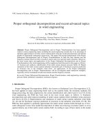
In addition, uniformity is assumed over the whole area swept by the rotor, and the speed of
the air beyond the rotor is considered to be axial. The ideal wind rotor is taken at rest and is
placed in a moving fluid atmosphere. Considering the ideal model shown in Fig. 1, the
cross sectional area swept by the turbine blade is designated as S, with the air cross-section
upwind from the rotor designated as S
1
, and downwind as S
2
.
The wind speed passing through the turbine rotor is considered uniform as V, with its value
as V
1
upwind, and as V
2

downwind at a distance from the rotor. Extraction of mechanical
energy by the rotor occurs by reducing the kinetic energy of the air stream from upwind to
downwind, or simply applying a braking action on the wind. This implies that:
21
VV

.
Consequently the air stream cross sectional area increases from upstream of the turbine to
the downstream location, and:
21
SS
.
If the air stream is considered as a case of incompressible flow, the conservation of mass or
continuity equation can be written as:

11 2 2
constantmSV SVSV

 

(2)
This expresses the fact that the mass flow rate is a constant along the wind stream.
Continuing with the derivation, Euler’s Theorem gives the force exerted by the wind on the
rotor as:

12
.( )
Fma
dV
m

dt
mV
SV V V






(3)
The incremental energy or the incremental work done in the wind stream is given by:
dE Fdx

(4)
From which the power content of the wind stream is:

Wind Turbines Theory - The Betz Equation and Optimal Rotor Tip Speed Ratio
21

dE dx
PFFV
dt dt
 
(5)
Substituting for the force F from Eqn. 3, we get for the extractable power from the wind:


Fig. 1. Pressure and speed variation in an ideal model of a wind turbine.
Pressure
P

2
P
1
P
3
Speed
V
2/3 V
1
1/3 V
1
V
S
V
1
S
1
V
2
S
2

Fundamental and Advanced Topics in Wind Power
22

2
12
.( )PSVVV



(6)
The power as the rate of change in kinetic energy from upstream to downstream is given by:


22
12
22
12
11
22
1
2
E
P
t
mV mV
t
mV V








(7)
Using the continuity equation (Eqn. 2), we can write:




22
12
1
2
PSVVV


(8)
Equating the two expressions for the power P in Eqns. 6 and 8, we get:



22 2
12 12
1
2
PSVVVSVVV



The last expression implies that:
22
12 1212
12
11
22
0
()()()
(), ,,

VV VVVV
VV V VS

  



or:

12 12 1 2
1
0
2
(),()VVVVV orVV 
(9)
This in turn suggests that the wind velocity at the rotor may be taken as the average of the
upstream and downstream wind velocities. It also implies that the turbine must act as a
brake, reducing the wind speed from V
1
to V
2
, but not totally reducing it to V = 0, at which
point the equation is no longer valid. To extract energy from the wind stream, its flow must
be maintained and not totally stopped.
The last result allows us to write new expressions for the force F and power P in terms of the
upstream and downstream velocities by substituting for the value of V as:

12
22
12

1
2
()
()
FSVVV
SV V





(10)






2
12
2
12 12
22
1212
1
4
1
4
PSVVV
SV V V V

SV V V V






(11)

Wind Turbines Theory - The Betz Equation and Optimal Rotor Tip Speed Ratio
23
We can introduce the “downstream velocity factor,” or “interference factor,” b as the ratio of
the downstream speed V
2
to the upstream speed V
1
as:

2
1
V
b
V

(12)
From Eqn. 10 the force F can be expressed as:

22
1
1

1
2
.( )FSVb


(13)
The extractable power P in terms of the interference factor b can be expressed as:





22
1212
32
1
1
4
1
11
4
PSVVVV
SV b b




(14)
The most important observation pertaining to wind power production is that the extractable
power from the wind is proportional to the cube of the upstream wind speed V

1
3
and is a
function of the interference factor b.
The “power flux” or rate of energy flow per unit area, sometimes referred to as “power
density” is defined using Eqn. 6 as:

3
3
22
1
2
1
2
'
,[ ],[ ]
.
P
P
S
SV
S
Joules Watts
V
ms m






(15)

The kinetic power content of the undisturbed upstream wind stream with V = V
1
and over a
cross sectional area S becomes:

32
1
2
1
2
,[ ],[ ]
.
Joules
W SV m Watts
ms

 (16)

The performance coefficient or efficiency is the dimensionless ratio of the extractable power
P to the kinetic power W available in the undisturbed stream:

p
P
C
W

(17)

The performance coefficient is a dimensionless measure of the efficiency of a wind turbine in
extracting the energy content of a wind stream. Substituting the expressions for P from Eqn.
14 and for W from Eqn. 16 we have:

Fundamental and Advanced Topics in Wind Power
24





32
1
3
1
2
1
11
4
1
2
1
11
2
p
P
C
W
SV b b
SV

bb






 
(18)




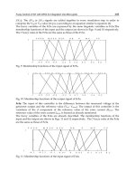
b
0.0 0.1 0.2 0.3 1/3 0.4 0.5 0.6 0.7 0.8 0.9 1.0
C
p

0.500 0.545 0.576 0.592 0.593 0.588 0.563 0.512 0.434 0.324 0.181 0.00
Fig. 2. The performance coefficient C
p
as a function of the interference factor b.
0
0.05
0.1
0.15
0.2
0.25
0.3
0.35

0.4
0.45
0.5
0.55
0.6
0 0.1 0.2 0.3 0.4 0.5 0.6 0.7 0.8 0.9 1
PerformancecoefficientC
p
Interferenceparameter,b

Wind Turbines Theory - The Betz Equation and Optimal Rotor Tip Speed Ratio
25
When b = 1, V
1
= V
2
and the wind stream is undisturbed, leading to a performance
coefficient of zero. When b = 0, V
1
= 0, the turbine stops all the air flow and the performance
coefficient is equal to 0.5. It can be noticed from the graph that the performance coefficient
reaches a maximum around b = 1/3.
A condition for maximum performance can be obtained by differentiation of Eq. 18 with
respect to the interference factor b. Applying the chain rule of differentiation (shown below)
and setting the derivative equal to zero yields Eq. 19:
()
ddvdu
uv u v
dx dx dx






2
2
22
2
1
11
2
1
121
2
1
122
2
1
13 2
2
1
13 1
2
0
[]
[]
()
()

()()
p
dC
d
bb
db db
bbb
bbb
bb
bb




 

(19)
Equation 19 has two solutions. The first is the trivial solution:
2
21
1
10
1
()
,
b
V
bVV
V




  

The second solution is the practical physical solution:

2
21
1
13 0
11
33
()
,
b
V
bVV
V



(20)
Equation 20 shows that for optimal operation, the downstream velocity V
2
should be equal
to one third of the upstream velocity V
1
. Using Eqn. 18, the maximum or optimal value of
the performance coefficient C
p

becomes:



2
2
1
11
2
11 1
11
23 3
16
27
0 59259
59 26
,
()
.
.
popt
Cbb
percent
 

 






(21)

Fundamental and Advanced Topics in Wind Power
26
This is referred to as the Betz Criterion or the Betz Limit. It was first formulated in 1919, and
applies to all wind turbine designs. It is the theoretical power fraction that can be extracted
from an ideal wind stream. Modern wind machines operate at a slightly lower practical
non-ideal performance coefficient. It is generally reported to be in the range of:

2
40
5
,.pprac
C percent
(22)
Result I
From Eqns. 9 and 20, there results that:

12
1
1
1
1
2
1
23
2
3
()

()
VVV
V
V
V



(23)
Result II
From the continuity Eqn. 2:

11 2 2
1
11
1
21 1
2
3
2
3
constant
S=S
S=S
mSV SVSV
V
S
V
V
S

V



 



(24)
This implies that the cross sectional area of the airstream downwind of the turbine expands
to 3 times the area upwind of it.
Some pitfalls in the derivation of the previous equations could inadvertently occur and are
worth pointing out. One can for instance try to define the power extraction from the wind
in two different ways. In the first approach, one can define the power extraction by an ideal
turbine from Eqns. 23, 24 as:
1
33
11 2 2
33
11 1 1
3
11
3
11
11
22
111
3
223
18

29
81
92
()
()
ideal upwind downwind
PP P
SV S V
SV S V
SV
SV










This suggests that fully 8/9 of the energy available in the upwind stream can be extracted by
the turbine. That is a confusing result since the upwind wind stream has a cross sectional
area that is smaller than the turbine intercepted area.

Wind Turbines Theory - The Betz Equation and Optimal Rotor Tip Speed Ratio
27
The second approach yields the correct result by redefining the power extraction at the wind
turbine using the area of the turbine as S = 3/2 S
1

:

3
11
3
1
3
1
3
1
18
29
182
293
116
227
16 1
27 2
()
()
()
ideal
PSV
SV
SV
SV









(25)
The value of the Betz coefficient suggests that a wind turbine can extract
at most 59.3
percent of the energy in an undisturbed wind stream.

16
0 592593 59 26
27
Betzcoe
ff
icient
p
ercent 
(26)
Considering the frictional losses, blade surface roughness, and mechanical imperfections,
between 35 to 40 percent of the power available in the wind is extractable under practical
conditions.
Another important perspective can be obtained by estimating the maximum power content
in a wind stream. For a constant upstream velocity, we can deduce an expression for the
maximum power content for a constant upstream velocity V
1
of the wind stream by
differentiating the expression for the power P with respect to the downstream wind speed
V
2
, applying the chain rule of differentiation and equating the result to zero as:






1
2
12 12
22
22
1212
2
22
12 212
22 2
12 12 2
22
12 12
1
4
1
4
1
2
4
1
22
4
1

32
4
0
[]
[]
[]
()
()
V
dP d
SVVVV
dV dV
d
SVVVV
dV
SV V V V V
SV V VV V
SV V VV











(27)

Solving the resulting equation by factoring it yield Eqn. 28.

22
1212
121 2
32 0
30
()
()( )
VVVV
VVV V
 

(28)
Equation 28 once again has two solutions. The trivial solution is shown in Eqn. 29.

Fundamental and Advanced Topics in Wind Power
28

12
21
0()VV
VV



(29)
The second physically practical solution is shown in Eqn 30.

12
21
30
1
3
()VV
VV



(30)
This implies the simple result that that the most efficient operation of a wind turbine occurs
when the downstream speed V
2
is one third of the upstream speed V
1
. Adopting the second
solution and substituting it in the expression for the power in Eqn. 16 we get the expression
for the maximum power that could be extracted from a wind stream as:



22
1212
2
2
11
11
3
1

3
1
1
4
1
493
111
11
493
16
27 2
max
[]
PSVVVV
VV
SV V
SV
VS Watt



















(31)

This expression constitutes the formula originally derived by Betz where the swept rotor
area S is:

2
4
D
S

 (32)
and the Betz Equation results as:

2
3
1
16
27 2 4
max
[]
D
PVWatt

 (33)

The most important implication from the Betz Equation is that there must be a wind speed
change from the upstream to the downstream in order to extract energy from the wind; in
fact by braking it using a wind turbine.
If no change in the wind speed occurs, energy cannot be efficiently extracted from the wind.
Realistically, no wind machine can totally bring the air to a total rest, and for a rotating
machine, there will always be some air flowing around it. Thus a wind machine can only
extract a fraction of the kinetic energy of the wind. The wind speed on the rotors at which
energy extraction is maximal has a magnitude lying between the upstream and downstream
wind velocities.
The Betz Criterion reminds us of the Carnot cycle efficiency in Thermodynamics suggesting
that a heat engine cannot extract all the energy from a given heat reservoir and must reject
part of its heat input back to the environment.

Wind Turbines Theory - The Betz Equation and Optimal Rotor Tip Speed Ratio
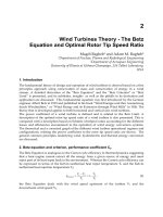
29

Fig. 3. Maximum power as a function of the rotor diameter and the wind speed. The power
increases as the square of the rotor diameter and more significantly as the cube of the wind
speed (Ragheb, M., 2011).
3. Rotor optimal Tip Speed Ratio, TSR
Another important concept relating to the power of wind turbines is the optimal tip speed
ratio, which is defined as the ratio of the speed of the rotor tip to the free stream wind speed.
If a rotor rotates too slowly, it allows too much wind to pass through undisturbed, and thus
does not extract as much as energy as it could, within the limits of the Betz Criterion, of
course.
On the other hand, if the rotor rotates too quickly, it appears to the wind as a large flat disc,
which creates a large amount of drag. The rotor Tip Speed Ratio, TSR depends on the blade
airfoil profile used, the number of blades, and the type of wind turbine. In general, three-
bladed wind turbines operate at a TSR of between 6 and 8, with 7 being the most widely-
reported value.

In addition to the factors mentioned above, other concerns dictate the TSR to which a wind
turbine is designed. In general, a high TSR is desirable, since it results in a high shaft
rotational speed that allows for efficient operation of an electrical generator. Disadvantages
however of a high TSR include:
a. Blade tips operating at 80 m/s of greater are subject to leading edge erosion from dust
and sand particles, and would require special leading edge treatments like helicopter
blades to mitigate such damage,
b. Noise, both audible and inaudible, is generated,
c. Vibration, especially in 2 or 1 blade rotors,
0
15
30
0
100
200
300
400
500
600
700
0
30
60
90
120
150
180
210
240
270

300
WindSpeed
[m/s]
MaximumPower[MW]
RotorDiameter[m]

Fundamental and Advanced Topics in Wind Power
30
d. Reduced rotor efficiency due to drag and tip losses,
e.
Higher speed rotors require much larger braking systems to prevent the rotor from
reaching a runaway condition that can cause disintegration of the turbine rotor blades.
The Tip Speed Ratio, TSR, is dimensionless factor defined in Eqn. 34

speed of rotor tip
TSR= =
wind speed
vr
VV


 (34)
where:
-1
wind speed [m/sec]
r rotor tip speed [m/sec]
rrotor radius [m]
=2 angular velocity [rad/sec]
rotational frequenc
y

[Hz], [sec ]
V
v
f
f








Example 1
At a wind speed of 15 m/sec, for a rotor blade radius of 10 m, rotating at 1 rotation per second:
1
22
210 20
20 62 83
4
15 15
rotation
[],
sec
radian
[]
sec
m
.[]
sec

.
f
f
vr
r
V
 
 




 

 

Example 2
The Suzlon S.66/1250, 1.25 MW rated power at 12 m/s rated wind speed wind turbine
design has a rotor diameter of 66 meters and a rotational speed of 13.9-20.8 rpm.
Its angular speed range is:
2
13 9 20 8
2
60
146 218
. . revolutions minute
[radian. . ]
minute second
radian
[ ]

sec
f








The range of its rotor’s tip speed can be estimated as:
66
146 218
2
48 18 71 94
(. . )
m
[]
sec
vr






Wind Turbines Theory - The Betz Equation and Optimal Rotor Tip Speed Ratio
31
The range of its tip speed ratio is thus:
48 18 71 94

12
46

r
V







The optimal TSR for maximum power extraction is inferred by relating the time taken for
the disturbed wind to reestablish itself to the time required for the next blade to move into
the location of the preceding blade. These times are t
w
and t
b
, respectively, and are shown
below in Eqns. 35 and 36. In Eqns. 35 and 36, n is the number of blades, ω is the rotational
frequency of the rotor, s is the length of the disturbed wind stream, and V is the wind
speed.

2
[sec]
s
t
n



 (35)

[sec]
w
s
t
V
 (36)
If t
s
> t
w
, some wind is unaffected. If t
w
> t
s
, some wind is not allowed to flow through the
rotor. The maximum power extraction occurs when the two times are approximately equal.
Setting t
w
equal to t
s
yields Eqn. 37 below, which is rearranged as:

22
sw
tt
sn
nVV s





 
(37)
Equation 37 may then be used to define the optimal rotational frequency as shown in Eqn. 38:

2
optimal
V
ns


 (38)
Consequently, for optimal power extraction, the rotor blade must rotate at a rotational
frequency that is related to the speed of the oncoming wind. This rotor rotational frequency
decreases as the radius of the rotor increases and can be characterized by calculating the
optimal TSR, λ
optimal
as shown in Eqn. 39.

2
optimal
optimal
r
r
Vns








(39)
4. Effect of the number of rotor blades on the Tip Speed Ratio, TSR
The optimal TSR depends on the number of rotor blades, n, of the wind turbine. The
smaller the number of rotor blades, the faster the wind turbine must rotate to extract the
maximum power from the wind. For an n-bladed rotor, it has empirically been observed
that s is approximately equal to 50 percent of the rotor radius. Thus by setting:

Fundamental and Advanced Topics in Wind Power
32
1
2
s
r

,
Eqn. 39 is modified into Eqn. 40:

24
optimal
r
ns n








(40)
For n = 2, the optimal TSR is calculated to be 6.28, while it is 4.19 for three-bladed rotor, and
it reduces to 3.14 for a four-bladed rotor. With proper airfoil design, the optimal TSR values
may be approximately 25 – 30 percent above these values. These highly-efficient rotor blade
airfoils increase the rotational speed of the blade, and thus generate more power. Using this
assumption, the optimal TSR for a three-bladed rotor would be in the range of 5.24 – 5.45.
Poorly designed rotor blades that yield too low of a TSR would cause the wind turbine to
exhibit a tendency to slow and stall. On the other hand, if the TSR is too high, the turbine
will rotate very rapidly, and will experience larger stresses, which may lead to catastrophic
failure in highly-turbulent wind conditions.
5. Power coefficient, C
p

The power generated by the kinetic energy of a free flowing wind stream is shown in Eqn.
41.

3
1
2
[]PSVWatt

 (41)
Defining the cross sectional area, S, of the wind turbine, in terms of the blade radius, r, Eqn.
41 becomes Eqn. 42.

23
1
2

PRV

 (42)
The power coefficient (Jones, B., 1950), Eqn. 43, is defined as the ratio of the power extracted
by the wind turbine relative to the energy available in the wind stream.

23
1
2
tt
p
PP
C
P
RV

 (43)
As derived earlier in this chapter, the maximum achievable power coefficient is 59.26
percent, the Betz Limit. In practice however, obtainable values of the power coefficient
center around 45 percent. This value below the theoretical limit is caused by the
inefficiencies and losses attributed to different configurations, rotor blades profiles, finite
wings, friction, and turbine designs. Figure 4 depicts the Betz, ideal constant, and actual
wind turbine power coefficient as a function of the TSR.
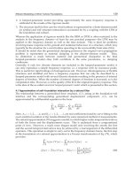
As shown in Fig. 4, maximum power extraction occurs at the optimal TSR, where the
difference between the actual TSR (blue curve) and the line defined by a constant TSR is the
lowest. This difference represents the power in the wind that is not captured by the wind
turbine. Frictional losses, finite wing size, and turbine design losses account for part of the


Wind Turbines Theory - The Betz Equation and Optimal Rotor Tip Speed Ratio

33

Fig. 4. Power coefficient as a function of TSR for a two-bladed rotor.
uncaptured wind power, and are supplemented by the fact that a wind turbine does not
operate at the optimal TSR across its operating range of wind speeds.
6. Inefficiencies and losses, Schmitz power coefficient
The inefficiencies and losses encountered in the operation of wind turbines include the
blade number losses, whirlpool losses, end losses and the airfoil profile losses (Çetin, N. S.
et. al. 2005).
Airfoil profile losses
The slip or slide number s is the ratio of the uplift force coefficient of the airfoil profile used
C
L
to the drag force coefficient C
D
is:

L
D
C
s
C

L
D
C
s
C
 (44)
Accounting for the drag force can be achieved by using the profile efficiency that is a

function of the slip number s and the tip speed ratio λ as:

1
profile
s
ss





1
profile
s
ss




(45)
Rotor tip end losses
At the tip of the rotor blade an air flow occurs from the lower side of the airfoil profile to the
upper side. This air flow couples with the incoming air flow to the blade. The combined air
flow results in a rotor tip end efficiency, η
tip end
.

Fundamental and Advanced Topics in Wind Power
34
Whirlpool Losses

In the idealized derivation of the Betz Equation, the wind does not change its direction after
it encounters the turbine rotor blades. In fact, it does change its direction after the
encounter.
This is accounted-for by a modified form of the power coefficient known as the Schmitz
power coefficient
C
pSchmitz
if the same airfoil design is used throughout the rotor blade.

Tip speed ratio
TSR
λ
Whirpool Schmitz
Power Coefficient
C
p
Schmitz

0.0 0.000
0.5 0.238
1.0 0.400
1.5 0.475
2.0 0.515
2.5 0.531
3.0 0.537
3.5 0.538
4.0 0.541
4.5 0.544
5.0 0.547
5.5 0.550

6.0 0.553
6.5 0.556
7.0 0.559
7.5 0.562
8.0 0.565
8.5 0.568
9.0 0.570
9.5 0.572
10.0 0.574
Table 1. Whirlpool losses Schmitz power coefficient as a function of the tip speed ratio.
Rotor blade number losses
A theory developed by Schmitz and Glauert applies to wind turbines with four or less rotor
blades. In a turbine with more than four blades, the air movement becomes too complex for
a strict theoretical treatment and an empirical approach is adopted. This can be accounted
for by a rotor blades number efficiency η
blades
.
In view of the associated losses and inefficiencies, the power coefficient can be expressed as:

pp
Schmitz
p
ro
f
ile ti
p
end blades
CC




(46)
There are still even more efficiencies involved:
1.
Frictional losses in the bearings and gears: η
friction


Wind Turbines Theory - The Betz Equation and Optimal Rotor Tip Speed Ratio
35

Fig. 5. Schmitz power coefficient as a function of the tip speed ratio, TSR.
2.
Magnetic drag and electrical resistance losses in the generator or alternator: η
electrical
.

'
p pSchmitz profile tip end blades friction electrical
CC

 

(47)
In the end, the Betz Limit is an idealization and a design goal that designers try to reach in a
real world turbine. A C
p
value of between 0.35 – 0.40 is a realistic design goal for a workable
wind turbine. This is still reduced by a capacity factor accounting for the periods of wind
flow as the intermittency factor.

7. Power coefficient and tip speed ratio of different wind converters designs
The theoretical maximum efficiency of a wind turbine is given by the Betz Limit, and is
around 59 percent. Practically, wind turbines operate below the Betz Limit. In Fig. 4 for a
two-bladed turbine, if it is operated at the optimal tip speed ratio of 6, its power coefficient
would be around 0.45. At the cut-in wind speed, the power coefficient is just 0.10, and at the
cut-out wind speed it is 0.22. This suggests that for maximum power extraction a wind
turbine should be operated around its optimal wind tip ratio.
Modern horizontal axis wind turbine rotors consist of two or three thin blades and are
designated as low solidity rotors. This implies a low fraction of the area swept by the rotors
being solid. Its configuration results in an optimum match to the frequency requirements of
modern electricity generators and also minimizes the size and weight of the gearbox or
transmission required, as well as increases efficiency.
Such an arrangement results in a relatively high tip speed ratio in comparison with rotors
with a high number of blades such as the highly successful American wind mill used for
water pumping in the American West and all over the world. The latter required a high
starting torque.
0
0.05
0.1
0.15
0.2
0.25
0.3
0.35
0.4
0.45
0.5
0.55
0.6
0246810

Schmitzpowercoefficient
TipSpeedratio,TSRλ

Fundamental and Advanced Topics in Wind Power
36
The relationship between the rotor power coefficient C
p
and the tip speed ratio is shown for
different types of wind machines. It can be noticed that it reaches a maximum at different
positions for different machine designs.


Fig. 6. The power coefficient C
p
as a function of the tip speed ratio for different wind
machines designs. Note that the efficiency curves of the Savonius and the American
multiblade designs were inadvertently switched (Eldridge, F. R., 1980) in some previous
publications, discouraging the study of the Savonius design.
The maximum efficiencies of the two bladed design, the Darrieus concept and the Savonius
reach levels above 30 percent but below the Betz Limit of 59 percent.
The American multiblade design and the historical Dutch four bladed designs peak at 15
percent. These are not suited for electrical generation but are ideal for water pumping.
8. Discussion and conclusions
Wind turbines must be designed to operate at their optimal wind tip speed ratio in order to
extract as much power as possible from the wind stream. When a rotor blade passes through
the air stream it leaves a turbulent wake in its path. If the next blade in the rotating rotor
arrives at the wake when the air is still turbulent, it will not be able to extract power from
the wind efficiently, and will be subjected to high vibration stresses. If the rotor rotated
slower, the air hitting each rotor blade would no longer be turbulent. This is another reason

Wind Turbines Theory - The Betz Equation and Optimal Rotor Tip Speed Ratio
37
for the tip speed ratio to be selected so that the rotor blades do not pass through turbulent
air.
Wind power conversion is analogous to other methods of energy conversion such as
hydroelectric generators and heat engines. Some common underlying basic principles can
guide the design and operation of wind energy conversion systems in particular, and of
other forms of energy conversion in general. A basic principle can be enunciated as:
“Energy can be extracted or converted only from a flow system.”
In hydraulics, the potential energy of water blocked behind a dam cannot be extracted
unless it is allowed to flow. In this case only a part of it can be extracted by a water turbine.
In a heat engine, the heat energy cannot be extracted from a totally insulated reservoir.
Only when it is allowed to flow from the high temperature reservoir, to a low temperature
one where it is rejected to the environment; can a fraction of this energy be extracted by a
heat engine.
Totally blocking a wind stream does not allow any energy extraction. Only by allowing the
wind stream to flow from a high speed region to a low speed region can energy be extracted
by a wind turbine.
A second principle of energy conversion can be elucidated as:
“Natural or artificial asymmetries in an aerodynamic, hydraulic, or thermodynamic system allow the
extraction of only a fraction of the available energy at a specified efficiency.”
Ingenious minds conceptualized devices that take advantage of existing natural
asymmetries, or created configurations or situations favoring the creation of these
asymmetries, to extract energy from the environment.
A corollary ensues that the existence of a flow system necessitates that only a fraction of the
available energy can be extracted at an efficiency characteristic of the energy extraction
process with the rest returned back to the environment to maintain the flow process.
In thermodynamics, the ideal heat cycle efficiency is expressed by the Carnot cycle
efficiency. In a wind stream, the ideal aerodynamic cycle efficiency is expressed by the Betz
Equation.

9. References
Ragheb, M., “Wind Power Systems. Harvesting the Wind.”
2011.
Thomas Ackerman, Ed. “Wind Power in Power Systems,” John Wiley and Sons, Ltd., 2005.
American Institute of Aeronautics and Astronautics (AIAA) and American Society of
Mechanical Engineers (ASME), “A Collection of the 2004 ASME Wind Energy
Symposium Technical Papers,” 42
nd
AIAA Aerospace Sciences Meeting and
Exhibit, Reno Nevada, 5-8 January, 2004.
Le Gouriérès Désiré, “Wind Power Plants, Theory and Design,” Pergamon Press, 1982.
Brown, J. E., Brown, A. E., “Harness the Wind, The Story of Windmills,” Dodd, Mead and
Company, New York, 1977.
Eldridge, F. R., “Wind Machines,” 2
nd
Ed., The MITRE Energy Resources and Environmental
Series, Van Nostrand Reinhold Company, 1980.
Calvert, N. G., “Windpower Principles: Their Application on the Small Scale,” John Wiley
and Sons, 1979.
Torrey, V., “Wind-Catchers, American Windmills of Yesterday and Tomorrow,” The
Stephen Greene Press, Brattleboro, Vermont, 1976.

Fundamental and Advanced Topics in Wind Power
38
Walker, J. F., Jenkins, N., “Wind Energy Technology,” John Wiley and Sons, 1997.
Schmidt, J., Palz, W., “European Wind Energy Technology, State of the Art Wind Energy
Converters in the European Community,” D. Reidel Publishing Company, 1986.
Energy Research and Development Administration (ERDA), Division of Solar Energy,
“Solar Program Assessment: Environmental Factors, Wind Energy Conversion,”
ERDA 77-47/6, UC-11, 59, 62, 63A, March 1977.

Çetin, N. S., M. A Yurdusev, R. Ata and A. Özdemir, “Assessment of Optimum Tip Speed
Ratio of Wind Turbines,” Mathematical and Computational Applications, Vol. 10,
No.1, pp.147-154, 2005.
Hau, E.,“Windkraftanlangen,” Springer Verlag, Berlin, Germany, pp. 110-113, 1996.
Jones, B., “Elements of Aerodynamics,” John Wiley and Sons, New York, USA, pp. 73-158,
1950.
3
Inboard Stall Delay Due to Rotation
Horia Dumitrescu and Vladimir Cardoş
Institute of Statistical Mathematics and Applied Mathematics of the Romanian Academy
Romania
1. Introduction

In the design process of improved rotor blades the need for accurate aerodynamic
predictions is very important. During the last years a large effort has gone into developing
CFD tools for prediction of wind turbine flows (Duque et al., 2003; Fletcher et al., 2009;
Sørensen et al.,2002). However, there are still some unclear aspects for engineers regarding
the practical application of CFD, such as computational domain size, reference system for
different computational blocks, mesh quality and mesh number, turbulence, etc. Thus, in the
design process and in the power curve prediction of wind turbines, the aerodynamic forces
are calculated with some form of the blade element method (BEM) and its extensions to the
three-dimensional wing aerodynamics. The results obtained by the standard methods are
reasonably accurate in the proximity of the design point, but in stalled condition the BEM is
known to underpredict the forces acting on the blades (Himmelskamp, 1947). The major
disadvantage of these methods is that the airflow is reduced to axial and circumferential
flow components (Glauert, 1963). Disregarding radial flow components present in the
bottom of separated boundary layers of rotating wings leads to alteration of lift and drag
characteristics of the individual blade sections with respect to the 2-D airfoils (Bjorck, 1995).
Airfoil characteristics of lift (C
L

) and drag (C
D
) coefficients are normally derived from two-
dimensional (2-D) wind tunnel tests. However, after stall the flow over the inboard half of
the rotor is strongly influenced by poorly understood 3-D effects (Banks & Gadd, 1963;
Tangler, 2002). The 3-D effects yield delayed stall with C
L
higher than 2.0 near the blade root
location and with correspondingly high C
D
. Now the design of constant speed, stall-
regulated wind turbines lacks adequate theory for predicting their peak and post-peak
power and loads.
During the development of stall-regulated wind turbines, there were several attempts to
predict 3-D post-stall airfoil characteristics (Corrigan & Schlichting, 1994; Du & Schling,
1998; Snel et al., 1993), but these methods predicted insufficient delayed stall in the root
region and tended to extend the delayed stall region too far out on the blade.
The present work aims at giving a conceptualization of the complex 3-D flow field on a rotor
blade, where stall begins and how it progresses, driven by the needs to formulate a
reasonably simple model that complements the 2-D airfoil characteristics used to predict
rotor performance.
Understanding wind turbine aerodynamics (Hansen & Butterfield, 1993) in all working
states is one of the key factors in making improved predictions of their performance. The
flow field associated with wind turbines is highly three-dimensional and the transition to
two-dimensional outboard separated flow is yet not well understood. A continued effort is

Fundamental and Advanced Topics in Wind Power

40
necessary to improve the delayed stall modeling and bring it to a point where the prediction

becomes acceptable. In the sequel, based on previous computed and measured results, a
comprehensible model is devised to explain in physical terms the different phenomena that
play a role and to clarify what can be modeled quantitatively in a scientific way and what is
possible in an engineering environment.
In 1945 Himmelskamp (Himmelskamp, 1947) first described through measurements the 3-D
and rotational effects on the boundary layer of a rotating propeller, finding lift coefficients
much higher moving towards the rotation axis. Further experimental studies confirmed
these early results, indicating in stall-delay and post-stalled higher lift coefficient values the
main effects of rotation on wings. Measurements on wind turbine blades were performed by
Ronstend (Ronsten, 1992), showing the differences between rotating and non-rotating
pressure coefficients and aerodynamic loads, and by Tangler and Kocurek (Tangler &
Kocurek, 1993), who combined results from measurements with the classical BEM method
to properly compute lift and drag coefficients and the rotor power in stalled conditions.
The theoretical foundations for the analysis of the rotational effects on rotating blades come
at the late 40’s with Sears (Sears, 1950), who derived a set of equations for the potential flow
field around a cylindrical blade of infinite span in pure rotation. He stated that the spanwise
component of velocity is dependent only upon the potential flow and it is independent of
the span (the so-called independence principle). Then, Fogarty and Sears (Fogarty & Sears,
1950) extended the former study to the potential flow around a rotating and advancing
blade. They confirmed that, for a cylindrical blade advancing like a propeller, the tangential
and axial velocity components are the same as in the 2-D motion at the local relative speed
and incidence. A more comprehensive work was made once more by Fogarty (Fogarty,
1951), consisting of numerical computations on the laminar boundary layer of a rotating
plate and blade with thickness. Here he showed that the separation line is unaffected by
rotation and that the spanwise velocities in the boundary layer appeared small compared to
the chordwise, and no large effects of rotation were observed in contrast to (Himmelskamp,
1947). A theoretical analysis done by Banks and Gadd (Banks &Gadd, 1963), focused on
demonstrating how rotation delays laminar separation. They found that the separation point
is postponed due to rotation, and for extreme inboard stations the boundary layer is
completely stabilized against separation.

In the NASA report done by McCroskey and Dwyer (McCroskey & Dwyer, 1969), the so-
called secondary effects in the laminar incompressible boundary layer of propeller and
helicopter rotor blades are widely studied, by means of a combined, numerical and
analytical approach. They showed that approaching the rotational axis, the Coriolis force in
the cross flow direction becomes more important. On the other hand the centrifugal
pumping effect is much weaker than was generally thought before, but its contribution
increases particularly in the region of the separated flow. The last two decades have known
the rising of computational fluid dynamics and the study of the boundary layer on rotating
blade has often been carried on through a numerical approach. Sørensen (Sørensen, 1986)
numerically solved the 3-D equations of the boundary layer on a rotating surface, using a
viscous-inviscid interaction model. In his results the position of the separation line still
appears the same as for 2-D predictions, but where separations are more pronounced a
larger difference between the lift coefficient calculated for the 2-D and 3-D case is noticed. A
quasi 3-D approach, based on the viscous-inviscid interaction method, was introduced by
Snel et al (Snel et al., 1993) and results were compared with measurements. They proposed a
semi-empirical law for the correction of the 2-D lift curve, identifying the local chord to radii

Inboard Stall Delay Due to Rotation

41
(c/r) ratio of the blade section as the main parameter of influence. This result has been
confirmed by Shen and Sørensen (Shen & Sørensen, 1999), and by Chaviaropoulos and
Hansen (Chaviaropoulos & Hansen, 2000), who performed airfoil computations applying a
quasi 3-D Navier-Stokes model, based on the streamfunction-vorticity formulation and
respectively a primitive variables form. Du and Seling (Du & Selling, 2000), and Dumitrescu
and Cardoş (Dumitrescu & Cardoş, 2010), investigated the effects of rotation on blade
boundary layers by solving the 3-D integral boundary-layer equations with the assumed
velocity profiles and a closure model. Dumitrescu and Cardoş studying the boundary layer
behavior very close to the rotation center (r/c < 1) stated that the stall delay depends
strongly on the leading edge separation bubbles formed on inboard blade segment due to a

suction effect at the root area of the blade (Dumitrescu & Cardoş, 2009).
Recently, with the advent of the supercomputer, computational fluid dynamics (CFD) tools
have been employed to investigate the stall-delay for wind turbines (Duque et al., 2003;
Fletcher et al., 2009; Sørensen et al., 2002). These calculations in addition to Narramore and
Vermeland’s results (Narramore & Vermeland, 1992) showed that the 3-D rotational effect
was particularly pronounced for the inboard sections, but the genesis of this phenomenon is
a problem still open. The present concern aims at giving explanations in physics terms of the
different features widely-observed experimentally and computationally in wind turbine
flow.
2. Flow at low wind speeds
At low wind speed conditions, i.e. at high speed ratios (TSR>3), the visualization of the
computed flow indicates that the flow is well-behaved and attached over much of the rotor,
Fig. 1. Figure 1 shows the separated area and radial flow on the suction side of a commercial
blade with 40 m length at the design tip speed ratio (TSR=5); the secondary flow is
strongest at approximately 0.17R and reaches up to 0.31R, where R is the rotor radius. The
local air velocity relative to a rotor blade consists of free-wind velocity V
w
defined as the
wind speed if there were no rotor present, that due to the blade motion 
b
r and the wake
induced velocities; at high TSR, a weak wake (Glauert, 1963) occurs and its rotational
induction velocity can be neglected. Wind turbine blade sections can operate in two main
flow regimes depending on the size of the rotation parameter defined as the ratio of wind
velocity to the local tangential velocity
/
wb
Vr

. If the rotation parameter is less than unity

along the entire span, and for properly twisted blades, the flow is mostly two-dimensional
and attached, while for rotation parameter greater than unity the flow is neither two-
dimensional nor steady, and is strongly affected by rotation. At high tip speed ratios the
subunitary
/
wb
Vr

condition is accomplished and the blade sections usually operate at
prestall incidences. Then, the boundary layer is attached all the way to the trailing edge on
the outside blade and is separated at trailing edge only on the inside blade, Fig. 1. At the
root area of the blade the flow close to the hub behaves like a rotating disk in a fluid at rest
(Fig. 2a), where the centrifugal forces induce a spinning motion in the separated flow; and a
radial velocity field is more or less uniform (Fig. 2b). Beginning at the hub, this secondary
flow generates the so-called centrifugal pumping mechanism, acting in separated trailing
edge flow. On the other hand, the Coriolis force acts in the chordwise direction as a
favorable pressure that mitigates separation at the trailing edge along the whole span.

Fundamental and Advanced Topics in Wind Power

42

Fig. 1. Typical surface and 3-D streamlines on the blade suction side at low wind speeds
(TSR=5)


Fig. 2. Pumping-work mode of a wind turbine at low wind speeds (TSR>3.0): a) conceptof
flow close to a rotating disk in a fluid at rest; b) model of the separation flow (Corten,
2001).
Therefore, at low wind speed, the main rotational effect is due to the Coriolis force which

delays the occurrence of separation to a point further downstream towards the trailing edge,
and by this the suction pressures move towards higher levels as r/c decreases. The pumping
effect is much weaker than was generally thought before.
The pressure field created by the presence of the turbine is related to the incoming flow field
around the blade, taken as being composed of the free wind velocity and the so-called
induction velocity due to the rotor and its wake. Thus, the incoming field results from a
weak interaction between two different flows: one axial and the other rotational

1/
wb
Vr . In such a weak interaction flow, the basic assumptions made are:

Inboard Stall Delay Due to Rotation

43
- the radial independence principle is applied to flow effects, i.e. induction velocities
used at a certain radial station depend only on the local aerodynamic forces at that
same station;
-
the mathematical description of the air flow over the blades is based on the 2-D flow
potential independent of the span, and on corrections for viscosity and 3-D rotational
effects.
These assumptions suitable to BEM methods reduce the complexity of the problem by an
order of magnitude yielding reliable results for the local forces and the overall torque in the
proximity of the design point, at high tip speed ratios. In order to estimate the 3-D rotational
effects, usually neglected in the traditional BEM model, the flow around a hypothetic blade
with prestall/stall incidence and chord constant along the whole span is considered in the
sequel.
2.1 Representation of flow elements
The set of equations including a simplified form of the inviscid flow and the full three-

dimensional boundary-layer equations are used to identify the influence of the3-D rotational
effects at low wind speeds.
A. Inviscid flow. In order to find the velocity at the airfoil surface in absence of viscous
effects, the reference velocity at a point on a rotating wind turbine blade is


2
2
1
rw
r
UV a
R






(1)
where V
w
is the wind speed,
b
w
R
V


 is the tip-speed ratio (TSR), R is the radius of the

turbine and a is the axial induced velocity interference, a function of the speed ratio 
(Burton et al., 2001). Starting from the idea of Fogarty and Sears (Fogarty & Sears, 1950), an
inviscid edge velocity can be calculated as


2,,
bb b
UrV Wr
z






   



(2)
where U, V and W represent the velocity components in the cylindrical coordinate system


,,rz

, which rotates with the blade with a constant-rotational speed 
b
(Fig. 3).



,z


denotes the 2-D potential solution, that is constant at all radial positions. The interesting
point regarding this set of equations (2) is that the spanwise component V can be derived
from the local 2-D velocity potential. However, this spanwise component is very small and
thus neglected in the present work. The potential edge velocity components can be
approached as

2
0,
erD
UUUV



(3)
where the non-dimensional velocity
2D
U could be obtained by a viscous-inviscid interaction
procedure for flow past a 2-D airfoil (Drela, 1989). Since the primary concern of the present
work is to investigate the rotational 3-D effects on prestalled and stalled blades by means of
the boundary layer method, the inviscid pressure distribution is simply considered as