Fundamental and Advanced Topics in Wind Power Part 6 pptx

Efficient Modelling of Wind Turbine Foundations 25
2. A lumped-parameter model providing approximately the same frequency response is
calibrated to the results of the rigorous model.
3. The structure itself (in this case the wind turbine) is represented by a finite-element model
(or similar) and soil–structure interaction is accounted for by a coupling with the LPM of
the foundation and subsoil.
Whereas the application of rigorous models like the BEM or DTM is often restricted to the
analysis in the frequency domain—at least for any practical purposes—the LPM may be
applied in the frequency domain as well as the time domain. This is ideal for problems
involving linear response in the ground and nonlinear behaviour of a structure, which may
typically be the situation for a wind turbine operating in the ser viceability limit state (SLS).
It should be noted that the geometrical damping present in the original wave-propagation
problem is represented as material damping in the discrete-element model. Thus,
no distinction is made between material and geometrical dissipation in the final
lumped-parameter model—they both contribute to the same parameters, i.e. damping
coefficients.
Generally, if only few discrete elements are included in the lumped-parameter model, it
can only reproduce a simple frequency response, i.e. a response with no resonance peaks.
This is useful for rigid footings on homogeneous soil. However, inhomogeneous or flexible
structures and stratified soil have a frequency response that can only be described by a
lumped-parameter model with several discrete elements resulting in the presence of internal
degrees of freedom. When the number of internal degrees of freedom is increased, so is the
computation time. However, so is the quality of the fit to the original frequency response. This
is the idea of the so-called consistent lumped-parameter model which is presented in this section.
4.1 Approximation of soil–foundation interaction by a rational filter
The relationship between a g eneralised force resultant, f (t), a cting at the foundation–soil
interface and the corresponding generalised displacement component, v
(t),canbe
approximated by a differential equation in the form:
k
∑

i=0
A
i
d
i
v(t)
dt
i
=
l
∑
j=0
B
j
d
j
f (t)
dt
j
. (79)
Here, A
i
, i = 1, 2, . . . , k,andB
j
, j = 1,2, ,l, are real coefficients found by curve fitting to the
exact analytical solution or the results obtained by some numerical method or measurements.
The rational approximation (79) suggests a model, in which higher-order temporal derivatives
of both the forces and the displacements occur. This is undesired from a computational
point of view. However, a much more elegant model only involving the zeroth, the first
and the second temporal derivatives may be achieved by a rearrangement of the differential

operators. This operation is simple to carry out in the frequency domain; hence, the first step
in the formulation of a rational approximation is a Fourier transformation of Eq. (79), which
provides:
k
∑
i=0
A
i
(iω)
i
V(ω)=
l
∑
j=0
B
j
(iω)
j
Q(ω) ⇒
Q(ω)=

Z
(iω)V(ω),

Z(iω)=
∑
k
i
=0
A

i
(iω)
i
∑
l
j
=0
B
j
(iω)
j
, (80)
139
Efficient Modelling of Wind Turbine Foundations
26 Will-be-set-by-IN-TECH
where V(ω) and F(ω) denote the complex amplitudes of the generalized displacements
and forces, respectively. It is noted that in Eq. (80) it has been assumed that the reaction
force F
(ω) stems from the response to a single displacement degree of freedom. This is
generally not the case. For example, as discussed in Section 3, there is a coupling between the
rocking moment–rotation and the horizontal force–translation of a rigid footing. However,
the model (80) is easily generalised to account for such behaviour by an extension in the form
F
i
(ω)=

Z
ij
(iω)V
j

(ω), where summation is carried out over index j equal to the degrees of
freedom contributing to the response. Each of the complex stiffness terms,

Z
ij
(iω),isgiven
by a polynomial fraction as illustrated by Eq. (80) for

Z
(iω). This forms the basis for the
derivation of so-called consistent lumped-parameter models.
4.2 Polynomial-fraction form of a rational filter
In the frequency domain, the dynamic stiffness related to a degree of freedom, or to the
interaction between two degrees of freedom, i and j,isgivenby

Z
ij
(a
0
)=Z
0
ij
S
ij
(a
0
) (no
sum on i, j). Here, Z
0
ij

= Z
ij
(0) denotes the static stiffness related to the interaction of the
two degrees of freedom, and a
0
= ωR
0
/c
0
is a dimensionless frequency with R
0
and c
0
denoting a characteristic length and wave velocity, respectively. For example, for a circular
footing with the radius R
0
on an elastic half-space with the S-wave velocity c
S
, a
0
= ωR
0
/c
S
may be chosen. With the given normalisation of the frequency it is noted that

Z
ij
(a
0

)=
Z
ij
(c
0
a
0
/R
0
)=Z
ij
(ω).
For simplicity, any indices indicating the degrees of freedom in q uestion are omitted in the
following subsections, e.g.

Z
(a
0
) ∼

Z
ij
(a
0
). The frequency-dependent stiffness coefficient
S
(a
0
) for a given degree of freedom is then decomposed into a s ingular part, S
s

(a
0
),anda
regular part, S
r
(a
0
),i.e.

Z
(a
0
)=Z
0
S(a
0
), S(a
0
)=S
s
(a
0
)+S
r
(a
0
), (81)
where Z
0
is the static stiffness, and the singular part has the form

S
s
(a
0
)=k
∞
+ ia
0
c
∞
. (82)
In this expression, k
∞
and c
∞
are two real-valued constants which are selected so that Z
0
S
s
(a
0
)
provides the entire stiffness in the high-frequency limit a
0
→ ∞. Typically, the stiffness
term Z
0
k
∞
vanishes and the complex stiffness in the high-frequency range becomes a pure

mechanical impedance, i.e. S
s
(a
0
)=ia
0
c
∞
. This is demonstrated in Section 5 for a two
different types of wind turbine foundations interacting with soil.
The regular part S
r
(a
0
) accounts for the remaining part of the stiffness. Generally, a
closed-form solution for S
r
(a
0
) is unavailable. Hence, the regular part of the complex
stiffness is usually obtained by fitting of a rational filter to the results obtained with a
numerical or semi-analytical model using, for example, the finite-element method (FEM), the
boundary-element method (BEM) or the domain-transformation method (DTM). Examples
are given in Section 5 for wind turbine foundations analysed by each of these methods.
Whether an analytical or a numerical solution is established, the output o f a frequency-domain
analysis is the complex dynamic stiffness

Z
(a
0

). T his is taken as the “target solution”, and the
regular part of the stiffness coefficient is found as S
r
(a
0
)=

Z
(a
0
)/Z
0
− S
s
(a
0
). A rational
approximation, or filter, is now introduced in the form
S
r
(a
0
) ≈

S
r
(ia
0
)=
P(ia

0
)
Q(ia
0
)
=
p
0
+ p
1
(ia
0
)+p
2
(ia
0
)
2
+ + p
N
(ia
0
)
N
q
0
+ q
1
(ia
0

)+q
2
(ia
0
)
2
+ + q
M
(ia
0
)
M
. (83)
140
Fundamental and Advanced Topics in Wind Power
Efficient Modelling of Wind Turbine Foundations 27
The orders, N and M, and the coefficients, p
n
(n = 0, 1, . . . , N)andq
m
(m = 0, 1, . . . , M), of
the numerator and denominator polynomials P
(ia
0
) and Q(i a
0
) are chosen according to the
following criteria:
1. To obtain a unique definition of the filter, one of the coefficients in either P
(ia

0
) or Q(ia
0
)
has to be given a fixed value. F or c onvenience, q
0
= 1 is chosen.
2. Since part of the static stiffness is already represented by S
s
(0)=k
∞
, t his part of the
stiffness should not be provided by S
r
(a
0
) as well. Therefore, p
0
/q
0
= p
0
= 1 −k
∞
.
3. In the high-frequency limit, S
(a
0
)=S
s

(a
0
). Thus, the regular part must satisfy the
condition that

S
r
(ia
0
) → 0fora
0
→ ∞.Hence,N < M, i.e. the num erator polynomial
P
(ia
0
) is at least one order lower than the denominator polynomial, Q(ia
0
).
Based on these criteria, Eq. (84) may advantageously be reformulated as
S
r
(a
0
) ≈

S
r
(ia
0
)=

P(ia
0
)
Q(ia
0
)
=
1 −k
∞
+ p
1
(ia
0
)+p
2
(ia
0
)
2
+ + p
M −1
(ia
0
)
M −1
1 + q
1
(ia
0
)+q

2
(ia
0
)
2
+ + q
M
(ia
0
)
M
. (84)
Evidently, the polynomial coefficients in Eq. (84) must provide a physically meaningful filter.
By a comparison with Eqs. (79 ) and (80) it follows that p
n
(n = 1,2, ,M − 1) and q
j
(m =
1, 2, . . . M) must all be real. Furthermore, no poles should appear along the positive real axis
as this will lead to an unstable solution in the time domain. This issue is discussed below.
The total approximation of S
(a
0
) is found by an addition of Eqs. (82) and (84) as stated in
Eq. (81). The approximation of S
(a
0
) has two important characteristics:
• It is exact in the static limit, since S
(a

0
) ≈

S
(ia
0
)+S
s
(a
0
) → 1fora
0
→ 0.
• It is exact in the high-frequency limit. Here, S
(a
0
) → S
s
(a
0
) for a
0
→ ∞ ,because

S
r
(ia
0
) →
0fora

0
→ ∞.
Hence, the approximation is double-asymptotic. For intermediate frequencies, the quality
of the fit depends on the order of the rational filter and the nature of the physical problem.
Thus, in some situations a low-order filter may provide a very good fit to the exact solution,
whereas other problems may require a high-order filter to ensure an adequate match—even
over a short range of frequencies. As discussed in the examples given below in Section 5, a
filter order of M
= 4 will typically provide satisfactory results for a footing on a homogeneous
half-space. However, for flexible, embedded foundations and layered soil, a higher order of
the filter may be necessary—even in the low-frequency range relevant to dynamic response of
wind turbines.
4.3 Partial-fraction form of a rational filter
Whereas the polynomial-fraction form is well-suited for curve fitting to measured or
computed responses, it provides little insight into the physics of the problem. To a limited
extent, such information is gained by a recasting of Eq. (84) into partial-fraction form,

S
r
(ia
0
)=
M
∑
m=1
R
m
ia
0
−s

m
, (85)
where s
m
, m = 1, 2, . . . , M, are the poles of

S
r
(ia
0
) (i.e. the roots of Q(ia
0
)), and R
j
are the
corresponding residues. The conversion of the original polynomial-fraction form into the
partial-fraction expansion form may be carried out in M
ATLAB with the built-in function
residue.
141
Efficient Modelling of Wind Turbine Foundations
28 Will-be-set-by-IN-TECH
The poles s
m
are generally complex. However, as discussed above, the coefficients q
m
must
be real in order to provide a rational approximation that is physically meaningful in the time
domain. To ensure this, any complex poles, s
m

, and the corresponding residues, R
m
,must
appear as conjugate pairs. When two such terms are added together, a second-order term
with real coefficients appears. Thus, with N conjugate pairs, Eq. (85) can be rewritten as

S
r
(ia
0
)=
N
∑
n=1
β
0n
+ β
1n
ia
0
α
0n
+ α
1n
ia
0
+(ia
0
)
2

+
M −N
∑
n=N+1
R
n
ia
0
−s
n
,2N ≤ M. (86)
The coefficients α
0n
, α
1n
, β
0n
and β
1n
, n = N + 1, N + 2, ,M − N,aregivenby
α
0n
= {s

n
}
2
+ {s

n

}
2
, α
1n
= −2s

n
, β
0n
= −2(R

n
s

n
+ R

n
s

n
), β
1n
= 2R

n
, (87)
where s

n

= (s
n
) and s

n
= (s
n
) are the real and imaginary parts of the complex conjugate
poles, respectively. Similarly, the real and imaginary parts of the complex conjugate residues
are denoted by R

n
= (R
n
) and R

n
= (R
n
), respectively.
By adding the singular term in Eq. (82) to the expression in Eq. (85), the total approximation
of the dynamic stiffness coefficient S
(a
0
) canbewrittenas

S
(ia
0
)=k

∞
+ ia
0
c
∞
+
N
∑
n=1
β
0n
+ β
1n
ia
0
α
0n
+ α
1n
ia
0
+(ia
0
)
2
+
M −N
∑
n=N+1
R

n
ia
0
−s
n
. (88)
The total approximation of the dynamic stiffness in Eq. (88) consists of three characteristic
types of terms, namely a constant/linear term, M
−2N first-order terms and N second-order
terms. These terms are given as:
Constant/linear term: k
∞
+ ia
0
c
∞
(89a)
First-order term:
R
ia
0
−s
(89b)
Second-order term:
β
1
ia
0
+ β
0

α
0
+ α
1
ia
0
+(ia
0
)
2
. (89c)
4.4 Physical interpretation of a rational filter
Now, each term in Eq. (89) may be identified as the frequency-response function for a
simple mechanical system consisting of springs, dashpots and point masses. Physically, the
summation of terms (88) may then be interpreted as a parallel coupling of M
− N + 1of
these so-called discrete-element models, and the resulting l umped-parameter model provides
a frequency-response function similar to that of the original continuous system. In the
subsections below, the calibration of the discrete-element models is discussed, and the
physical interpretation of each kind of term in Eq. (89) is described in detail.
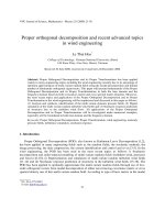
4.4.1 Constant/linear term
The constant/linear term given by Eq. (89a) consists of t wo known parameters, k
∞
and c
∞
,
that represent the singular part of the dynamic stiffness. The discrete-element model for the
constant/linear term is shown in Fig. 9.
The equilibrium formulation of Node 0 (for harmonic loading) is as follows:
κU

0
(ω)+i ωγ
R
0
c
0
U
0
(ω)=P
0
(ω) (90)
142
Fundamental and Advanced Topics in Wind Power
Efficient Modelling of Wind Turbine Foundations 29
P
0
U
0
κ
γ
R
0
c
0
0
Fig. 9. The discrete-element model for the constant/linear term.
Recalling that the dimensionless frequency is introduced as a
0
= ωR
0

/c
0
, the equilibrium
formulation in Eq. (90) results in a force–displacement relation given by
P
0
(a
0
)=
(
κ + ia
0
γ
)
U
0
(a
0
). (91)
By a comparison of Eqs. (89a) and (91) it becomes evident that the non-dimensional
coefficients κ and γ are equal to k
∞
and c
∞
, respectively.
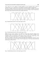
4.4.2 First-order terms with a single internal degree of freedom
The first-order term given by Equation (89b) has two parameters, R and s.Thelayoutofthe
discrete-element model is s hown i n Fig. 10a. The model i s constructed by a spring (
−κ)in
parallel with another spring (κ)anddashpot(γ

R
0
c
0
) in series. The serial connection between
the spring (κ) and the dashpot (γ
R
0
c
0
) results in an internal node (internal degree of freedom).
The equilibrium formulations for Nodes 0 and 1 (for harmonic loading) are as follows:
Node 0 : κ

U
0
(ω) −U
1
(ω)

−κU
0
(ω)=P
0
(ω) (92a)
Node 1 : κ

U
1
(ω) −U

0
(ω)

+ iωγ
R
0
c
0
U
1
(ω)=0. (92b)
After elimination of U
1
(ω) in Eqs. (92a) a nd (92b), it becomes cl ear that the force–displacement
relation of the first-order model is given as
P
0
(a
0
)=
−
κ
2
γ
ia
0
+
κ
γ
U

0
(a
0
). (93)
By comparing Eqs. (89b) and (93), κ and γ are identified as
κ
=
R
s
, γ
= −
R
s
2
. (94)
0
0
1
1
P
0
P
0
U
0
U
0
U
1
U

1
−κ
κ
γ
L
c
γ
L
c
−γ
L
c
γ
2


L
2
c
2
(a) (b)
Fig. 10. The discrete-element model for the first-order term: (a) Spring-dashpot model;
(b) monkey-tail model.
143
Efficient Modelling of Wind Turbine Foundations
30 Will-be-set-by-IN-TECH
It should be noted that the first-order term could also be represented by a so-called
“monkey-tail” model, see Fig. 10b. This turns out to be advantageous in situations where
κ and γ in Eq. (94) are negative, which may be the case when R is positive (s is negative). To
avoid negative coefficients of springs and dashpots, the monkey-tail model is applied, and

the resulting coefficients are positive. By inspecting the equilibrium formulations for Nodes 0
and 1, see Fig. 10b, the coefficients can be identified as
γ
=
R
s
2
,  = −
R
s
3
. (95)
Evidently, the internal degree of freedom in the monkey-tail model has no direct physical
meaning in relation to the original problem providing the target solution. Thus, at low
frequencies the point mass may undergo extreme displacements, and in the static case the
displacement is infinite. This lack of direct relationship with the original problem is a general
property of the discrete-element models. They merely provide a mechanical system that leads
to a similar frequency response.
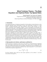
4.4.3 Second-order terms with one or two internal degrees of fredom
The second-order term given by Eq. (89c) has four parameters: α
0
, α
1
, β
0
and β
1
.Anexample
of a second-order discrete-element model is shown in Fig. 11a. This particular model has two
internal nodes. The equilibrium formulations for Nodes 0, 1 and 2 (for harmonic loading) are

as follows:
Node 0 : κ
1

U
0
(ω) −U
1
(ω)

−κ
1
U
0
(ω)=P
0
(ω) (96a)
Node 1 : κ
1

U
1
(ω) −U
0
(ω)

+ iωγ
1
R
0

c
0

U
1
(ω) −U
2
(ω)

= 0 (96b)
Node 2 : κ
2
U
2
(ω)+iωγ
2
R
0
c
0
U
2
(ω)+iωγ
1
R
0
c
0

U

2
(ω) −U
1
(ω)

= 0. (96c)
After some rearrangement and elimination of the internal degrees of freedom, the
force-displacement relation of the second-order model is given by
P
0
(a
0
)=
−
κ
2
1
γ
1
+γ
2
γ
1
γ
2
ia
0
−
κ
2

1
κ
2
γ
1
γ
2
(ia
0
)
2
+

κ
1
γ
1
+γ
2
γ
1
γ
2
+
κ
2
γ
2

ia

0
+
κ
1
κ
2
γ
1
γ
2
U
0
(a
0
). (97)
0
0
1
1
2
P
0
P
0
U
0
U
0
U
1

U
1
U
2
γ
L
c
γ
L
c
γ
1
L
c
γ
2
L
c
−γ
L
c
−κ
1
+
γ
2

κ
1
κ

1
−κ
1
κ
2
κ
2

L
2
c
2
(a)
(b)
Fig. 11. The discrete-element model for the second-order term: (a) Spring-dashpot model
with two internal degrees of freedom; (b) spring-dashpot-mass model with one internal
degree of freedom.
144
Fundamental and Advanced Topics in Wind Power
Efficient Modelling of Wind Turbine Foundations 31
By a comparison of Eqs. (89c) and (97), the four coefficients in Eq. (97) are identified as
κ
1
= −
β
0
α
0
, γ
1

= −
α
0
β
1
−α
1
β
0
α
2
0
, (98a)
κ
2
=
β
0
α
2
0
(−α
0
β
1
+ α
1
β
0
)

2
α
0
β
2
1
−α
1
β
0
β
1
+ β
2
0
, γ
2
=
β
2
0
α
2
0
−α
0
β
1
+ α
1

β
0
α
0
β
2
1
−α
1
β
0
β
1
+ β
2
0
. (98b)
Alternatively, introducing a second-order model with springs, dampers and a point mass, it
is possible to construct a second-order model with only one internal degree of freedom. The
model is sketched in Fig. 11b. The force–displacement relation of the alternative second-order
model is given by
P
0
(a
0
)=
2

κ
1

γ

+
γ
3

2

ia
0
−
κ
2
1

+
(κ
1
+κ
2
)γ
2

2
(ia
0
)
2
+ 2
γ


ia
0
+
κ
1
+κ
2

U
0
(a
0
). (99)
By equating the coefficients in Eq. (99) to the terms of the second-order model in Eq. (89c),
the four parameters κ
1
, κ
2
, γ and  can be determined. In order to calculate , a quadratic
equation has to be solved. The quadratic equation for  is
a
2
+ b + c = 0wherea = α
4
1
−4α
0
α
2

1
, b = −8α
1
β
1
+ 16β
0
, c = 16
β
2
1
α
2
1
. (100)
Equation (100) results in two solutions for . To ensure real values of , b
2
− 4ac ≥ 0or
α
0
β
2
1
− α
1
β
0
β
1
+ β

2
0
≥ 0. When  has been determined, the three remaining coefficients can
be calculated by
κ
1
=
α
2
1
4
−
β
1
α
1
, κ
2
= α
0
−κ
1
, γ =
α
1
2
. (101)
4.5 Fitting of a rational filter
In order to get a stable solution in the time d omain, the poles o f


S
r
(ia
0
) should all reside in
the second and third quadrant of the complex plane, i.e. the real parts of the p oles must al l
be negative. Due to the fact that computers only have a finite precision, this requirement m ay
have to be adjusted to s
m
< −ε, m = 1, 2, . . . , M ,whereε is a small number, e.g. 0.01.
The rational approximation may now be obtained by curve-fitting of the rational filter

S
r
(ia
0
)
to the regular part of the dynamic stiffness, S
r
(a
0
), by a least-squares technique. In this
process, it should be observed that:
1. The response should be accurately described by the lumped-parameter model in the
frequency range that is important for the physical problem being investigated. For
soil–structure interaction of wind turbines, this is typically the low-frequency range.
2. The “exact” values of S
r
(a
0

) are only measured—or computed—over a finite range of
frequencies, typically for a
0
∈
[
0; a
0max
]
with a
0max
= 2 ∼ 10. Further, the values of
S
r
(a
0
) are typically only known at a number of discrete frequencies.
3. Outside the frequency range, in which S
r
(a
0
) has been provided, the singular part of the
dynamic stiffness, S
s
(a
0
), should govern the response. Hence, no additional tips and
dips should ap pear in the frequency response provided by the rational filter beyond the
dimensionless frequency a
0max
.

145
Efficient Modelling of Wind Turbine Foundations
32 Will-be-set-by-IN-TECH
Firstly, this implies that the order of the filter, M, should not be too high. Experience shows
that or ders about M
= 2 ∼ 8 are adequate for most physical problems. Higher-order filters
than this are not easily fitted, and lower-order filters provide a poor match to the “exact”
results. Secondly, in order to ensure a good fit of

S
r
(ia
0
) to S
r
(a
0
) in the low-frequency range,
it is recommended to employ a higher weight on the squared errors in the low-frequency
range, e.g. for a
0
< 0.2 ∼ 2, compared with the weights in the medium-to-high-frequency
range. Obviously, the definition of low, medium and high frequencies is strongly dependent
on the problem in question. For example, frequencies that are considered high for an offshore
wind turbine, may be considered low for a diesel power generator.
For soil-structure interaction of foundations, Wolf (1994) suggested to employ a weight of
w
(a
0
)=10

3
∼ 10
5
at low frequencies and unit weight at higher frequencies. This should
lead to a good approximation in most cases. However, numerical experiment indicates t hat
the fitting goodness of the rational filter is h ighly sensitive to the choice of the weight function
w
(a
0
), and the guidelines provided by Wolf (1994) are not useful in all situations. Hence, as
an alternative, the following fairly general weight function is proposed:
w
(a
0
)=
1

1
+
(
ς
1
a
0
)
ς
2

ς
3

. (102)
The coefficients ς
1
, ς
2
and ς
3
are heuristic parameters. Experience shows that values of about
ς
1
= ς
2
= ς
3
= 2 provide an adequate solution f or most foundations in the low-frequency
range a
0
∈
[
0; 2
]
. This recommendation is justified by the examples given in the next section.
For analyses involving high-frequency excitation, lower values of ς
1
, ς
2
and ς
3
may have to
be employed.

Hence, the optimisation p r oblem defined in Table 1. However, the requirement of all poles
lying in the second and third quadrant of the complex plane is not easily fulfilled when an
optimisation is carried out by least-squares (or similar) curve fitting of

S
r
(ia
0
) to S
r
(a
0
) as
suggested in Table 1. Specifically, the choice of the polynomial coefficients q
j
, j = 1, 2, . . . , m,
as the optimisation variables is unsuitable, since the constraint that all poles of

S
r
(ia
0
) must
have negative real parts is not easily incorporated in the optimisation problem. Therefore,
instead of the interpretation
Q
(ia
0
)=1 + q
1

(ia
0
)+q
2
(ia
0
)
2
+ + q
M
(ia
0
)
M
, (103)
an alternative approach is considered, in which the denominator is expressed as
Q
(ia
0
)=(ia
0
−s
1
)(ia
0
−s
2
) ···(ia
0
−s

M
)=
M
∏
m=1
(ia
0
−s
m
). (104)
In this representation, s
m
, m = 1,2, ,M, are the roots of Q(ia
0
). In particular, if there are N
complex conjugate pairs, the denominator polynomial may advantageously be expressed as
Q
(ia
0
)=
N
∏
n=1
(
ia
0
−s
n
)(
ia

0
−s
∗
n
)
·
M −N
∏
n=N+1
(
ia
0
−s
n
)
. (105)
where an asterisk (
∗) denotes the complex conjugate. Thus, instead of the polynomial
coefficients, the roots s
n
are identified as the optimisation variables.
146
Fundamental and Advanced Topics in Wind Power
Efficient Modelling of Wind Turbine Foundations 33
A rational filter for the regular part of the dynamic stiffness is defined in the form:
S
r
(a
0
) ≈


S
r
(ia
0
)=
P(ia
0
)
Q(ia
0
)
=
1 − k
∞
+ p
1
(ia
0
)+p
2
(ia
0
)
2
+ + p
M−1
(ia
0
)

M−1
1 + q
1
(ia
0
)+q
2
(ia
0
)
2
+ + q
M
(ia
0
)
M
.
Find the optimal polynomial coefficients p
n
and q
m
which minimize the object function F(p
n
, q
m
) in a
weighted-least-squares sense subject to the constraints G
1
(p

n
, q
m
), G
2
(p
n
, q
m
), ,G
M
(p
n
, q
m
).
Input: M : order of the filter
p
0
n
, n = 1, 2, . . . , M − 1,
q
0
m
, m = 1, 2, . . ., M,
a
0j
, j = 1, 2, . . . , J,
S
r

(a
0j
), j = 1, 2, . . . , J,
w
(a
0j
), j = 1, 2, . . . , J.
Var iables: p
n
, n = 1, 2, . . . , M − 1,
q
m
, m = 1, 2, . . ., M.
Object function: F
(p
n
, q
m
)=
∑
J
j
=1
w(a
0j
)


S
r

(ia
0j
) −S
r
(a
0j
)

2
.
Constraints: G
1
(p
n
, q
m
)=(s
1
) < −ε,
G
2
(p
n
, q
m
)=(s
2
) < −ε,
.
.

.
G
M
(p
n
, q
m
)=(s
M
) < −ε.
Output: p
n
, n = 1, 2, . . . , M − 1,
q
m
, m = 1, 2, . . ., M.
Here, p
0
n
and q
0
m
are the initial values of the polynomial coefficients p
n
and q
m
,whereasS
r
(a
0j

) are the
“exact” value of the dynamic stiffness evaluated at the J discrete dimensionless frequencies a
0j
.These
are either measured or calculated by rigourous numerical or analytical methods. Further,

S
r
(ia
0j
) are
the values of the rational filter at the same discrete frequencies, and w
(a
0
) is a weight function, e.g. as
defined by Eq. (102) with ς
1
= ς
2
= ς
3
= 2. Finally, s
m
are the poles of the rational filter

S
r
(ia
0
),

i.e. the roots of the denominator polynomial Q
(ia
0
),andε is a small number, e.g. ε = 0.01.
Table 1. Fitting of rational filter by optimisation of polynomial coefficients.
Accordingly, in addition to the coefficients of the numerator polynomial P
(ia
0
),thevariables
in the optimisation problem are the real and i maginary parts s

n
= (s
n
) and s

n
= (s
n
) of
the complex roots s
n
, n = 1, 2, . . . , N, and the real roots s
n
, n = N + 1, N + 2, ,M − N.
The great advantage of the representation (105) is that the constraints on the poles are
defined directly on each individual variable, whereas the constraints in the formulation
with Q
(ia
0

) defined by Eq. (103), the constraints are given on functionals of the variables.
Hence, the solution is much more efficient and s traightforward. However, Eq. (105) has two
disadvantages when compared with Eq. (103):
• The number of complex conjugate pairs has to be estimated. However, experience shows
that as many as possible of the roots should appear as complex conjugates—e.g. if M is
even, N
= M/ 2 should be utilized. This provides a good fit in most situations and
may, at the same time, generate the lumped-parameter model with fewest possible internal
degrees of freedom.
147
Efficient Modelling of Wind Turbine Foundations
34 Will-be-set-by-IN-TECH
A rational filter for the regular part of the dynamic stiffness is defined in the form:
S
r
(a
0
) ≈

S
r
(ia
0
)=
P(ia
0
)
Q(ia
0
)

=
1 − k
∞
+ p
1
(ia
0
)+p
2
(ia
0
)
2
+ + p
M−1
(ia
0
)
M−1
∏
N
m
=1
(
ia
0
−s
m
)(
ia

0
− s
∗
m
)
·
∏
M−N
m
=N+1
(
ia
0
−s
m
)
.
Find the optimal polynomial coefficients p
n
and the poles s
m
which minimise the object function
F
(p
n
, s
m
) subject to the constraints G
0
(p

n
, s
m
), G
1
(p
n
, s
m
), ,G
N
(p
n
, s
m
).
Input: M : order of the filter
N : number of complex conjugate pairs, 2N
≤ M
p
0
n
, n = 1,2, ,M −1,
s
0
m
, m = 1,2, ,N,
s
0
m

, m = 1,2, ,N,
s
0
m
, m = 1,2, ,M −N,
a
0j
, j = 1,2, ,J,
S
r
(a
0j
), j = 1,2, ,J,
w
(a
0j
), j = 1,2, ,J.
Var iables: p
n
, n = 1,2, ,M −1,
s

m
, m = 1,2, ,N, s

m
< −ε,
s

m

, m = 1,2, ,N, s

m
> +ε,
s
m
, m = N + 1,2, ,M −N, s
m
< −ε.
Object function: F
(p
n
, s
m
)=
∑
J
j
=1
w(a
0j
)


S
r
(ia
0j
) − S
r

(a
0j
)

2
.
Constraints: G
0
(p
n
, s
m
)=1 −
∏
M
1
(
−
s
m
)
=
0,
G
k
(p
n
, s
m
)=ζs


k
+ s

k
< 0, k = 1,2, ,N.
Output: p
n
, n = 1,2, ,M −1,
s

m
, m = 1,2, ,N,
s

m
, m = 1,2, ,N,
s
m
, m = N + 1,2, ,M −N.
Here, superscript 0 indicates initial values of the respective variables, and

S
r
(ia
0j
) are the values of
the rational filter at the same discrete frequencies. Further, ζ
≈ 10 ∼ 100 and ε ≈ 0.01 are two real
parameters. Note that the initial values of the poles must conform with the constraint G

0
(p
n
, s
m
).For
additional information, see Table 1.
Table 2. Fitting of rational filter by optimisation of the poles.
• In the representation provided by Eq. (103), the correct asymptotic behaviour is
automatically ensured in the limit i a
0
→ 0, i.e. the static case, since q
0
= 1.
Unfortunately, in the representation given by Eq. (105) an additional equality constraint
has to be implemented to ensure this behaviour. However, this condition is much easier
implemented than the constraints which are necessary in the case o f Eq. (103) in order to
prevent the real parts of the roots from being positive.
Eventually, instead of the problem defined in Table 1, it may be more efficient t o solve the
optimisation problem given in Table 2 . It is noted that additional constraints are suggested,
which prevent the imaginary parts of the complex poles to become much (e.g. 10 times) bigg e r
than the real parts. This i s due to the following reason: If the real part of the complex pole
s
m
vanishes, i.e. s

m
= 0, this results in a second order pole, {s

m

}
2
, which is real and positive.
148
Fundamental and Advanced Topics in Wind Power
Efficient Modelling of Wind Turbine Foundations 35
Evidently, this will lead to instability in the time domain. Since the computer precision is
limited, a real part of a certain size compared to the imaginary part of the pole is necessary to
ensure a stable solution.
Finally, as an alternative to the optimisation problems defined in Table 1 and Table 2, the
function S
(ia
0
) may be expressed b y Eq. (86), i.e. in partial-fraction form. I n this case, the
variables in the optimization problem are the poles and residues of S
(ia
0
).Inthecaseofthe
second-order terms, these quantities are replaced with α
0
, α
1
, β
0
and β
1
. Atafirstglance,
this choice of optimisation variable seems more natural than p
n
and s

m
, as suggested in
Table 2. However, from a computational point of view, the mathematical operations involved
in the polynomial-fraction form are more efficient than those of the polynomial-fraction form.
Hence, the scheme provided in Table 2 is recommended.
5. Time-domain analysis of soil–structure interaction
In this section, two examples are given in which consistent lumped-parameter models
are applied to the analysis of foundations and soil–structure interaction. T he first
example concerns a rigid hexagonal footing on a homogeneous or layered ground and
was first presented by Andersen (2010). The frequency-domain solution obtained by the
domain-transformation method p resented in Sections 2–3 is fitted by LPMs of different orders.
Subsequently, the response o f the original model and the LPMs are compared in f requency and
time domain.
In the second example, originally proposed by Andersen et al. ( 2009), LPMs are fitted to the
frequency-domain results of a coupled boundary-element/finite-element model of a flexible
embedded foundation. As part of the examples, the complex stiffness of the foundation in the
high-frequency limit is discussed, i.e. the coefficients k
∞
and c
∞
in Eq. (82) are determined for
each component of translation and rotation of the foundation. Whereas no coupling exists
between horizontal sliding and rocking of surface footings in the high-frequency limit, a
significant coupling is present in the case of e mbedded foundations—even at high frequencies.
5.1 Example: A footing on a homogeneous or layered ground
The foundation is modelled as a regular hexagonal rigid footing with the side length r
0
,height
h
0

and mass density ρ
0
. This geometry is typical for offshore wind turbine foundations.
x
1
x
2
x
3
r
0
h
0
Free surface
Layer 1
Layer 2
Half-space
Fig. 12. Hexagonal footing on a stratum with three layers over a half-space.
149
Efficient Modelling of Wind Turbine Foundations
36 Will-be-set-by-IN-TECH
As illustrated in Fig. 12, the centre of the soil–foundation interface coincides with the origin
of the Cartesian coordinate system. The mass of the foundation and the corresponding mass
moments of inertia with respect to the three coordinate axes then become:
M
0
= ρ
0
h
0

A
0
, J
1
= J
2
= ρ
0
h
0
I
0
+
1
3
ρ
0
h
3
0
A
0
, J
3
= 2ρ
0
h
0
I
0

, (106a)
where A
0
is the area of the horizontal cross-section and I
0
is the corresponding geometrical
moment of inertia,
A
0
=
3
√
3
2
r
2
0
, I
0
=
5
√
3
16
r
4
0
. (106b)
It is noted that
I

0
is invariant to rotation of the foundation around the x
3
-axis. This property
also applies to circular or quadratic foundations as discussed in Section 3.
5.1.1 A footing on a homogeneous ground
Firstly, we consider a hexagonal footing on a homogeneous visco-elastic half-space. The
footing has the side length r
0
= 10 m, the height h
0
= 10 m and the mass density
ρ
0
= 2000 kg/m
3
, and the mass and mass moments of inertia are computed by Eq. (106).
The properties of the soil are ρ
1
= 2000 kg/m
3
, E
1
= 10
4
kPa, ν
1
= 0.25 and η
1
= 0.03.

However, in the static limit, i.e. for ω
→ 0, the hysteretic damping model leads to a complex
impedance in the frequency domain. By contrast, the lumped-parameter model provides a
real impedance, since it is based o n viscous dashpots. This discrepancy leads to numerical
difficulties in the fitting procedure and to overcome this, the hysteretic damping model for
the soil is replaced by a linear viscous model at low frequencies, in this case below 1 Hz.
In principle, the time-domain solution for the displacements and rotations of the rigid footing
is found by inverse Fourier transformation, i.e.
v
i
(t)=
1
2π

∞
−∞
V
i
(ω)e
iωt
dω, θ
i
(t)=
1
2π

∞
−∞
Θ
i

(ω)e
iωt
dω, i = 1, 2, 3. (107)
The displacements, rotations, forces and moments in the time domain are visualised in
Fig. 13. In the numerical computations, the frequency response spectrum is discretized and
accordingly, the time-domain solution is found by a Fourier series.
According to Eqs. (72) and (74), the vertical motion V
3
(ω) as well as the torsional motion
Θ
3
(ω) (see Fig. 6) are decoupled from the remaining degrees of freedom of the hexagonal
footing. Thus, V
3
(ω) and Θ
3
(ω) may be fitted by independent lumped-parameter models.
x
1
x
1
x
2
x
2
x
3
x
3
θ

1
θ
2
θ
3
v
1
v
2
v
3
m
1
m
2
m
3
q
1
q
2
q
3
(a)
(b)
Fig. 13. Degrees of freedom for a rigid surface footing in the time domain: (a) displacements
and rotations, and (b) forces and moments.
150
Fundamental and Advanced Topics in Wind Power
Efficient Modelling of Wind Turbine Foundations 37

In the following, the quality of lumped-parameter models based on rational filters of different
orders are tested for vertical and torsional excitation.
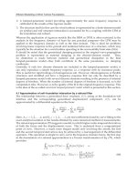
For the footing on the homogeneous half-space, rational filters of the order 2–6 are tested.
Firstly, the impedance components are determined i n the frequency-domain by the me thod
presented in Section 2. The lumped-parameter models are then fitted by application of the
procedure described in Section 4 and summarised in Table 2. The two components of the
normalised impedance, S
33
and S
66
, are shown in Figs. 14 and 16 as functions of the physical
frequency, f . I t is noted that all the LPMs are based on second-order discrete-element models
including a point mass, see Fig. 11b. Hence, the LPM for each individual component of the
impedance matrix, Z
(ω), has 1, 2 or 3 internal degrees of freedom.
With reference to Fig. 14, a poor fit of the vertical impedance is obtained with M
= 2
regarding the absolute value of S
33
as well as the phase angle. A lumped-parameter model
with M
= 4 provides a much better fit in the low-frequency range. However, a sixth-order
lumped-parameter model is required to obtain an accurate solution in the medium-frequency
range, i.e. for frequencies between approximately 1.5 and 4 Hz. As expected, further analyses
show that a slightly better match in the medium-frequency range is obtained with the
weight-function coefficients ς
1
= 2andς
2
= ς

3
= 1. However, this comes at the cost of a
poorer match in the low-frequency range. Finally, it has been found that no improvement is
achieved if first-order terms, e.g. the “monkey tail” illustrated in Fig. 10b, are allowed in the
rational-filter approximation.
Figure 16 shows the rational-filter approximations of S
66
, i.e. t he non-dimensional to rsional
impedance. Compared with the results for the vertical impedance, the overall quality of the fit
is relatively poor. In particular the LPM with M
= 2 provides a phase angle which is negative
in the low frequency range. Actually, this means that the geometrical damping provided
by the second-order LPM becomes negative for low-frequency excitation. Furthermore, the
stiffness is generally under-predicted and as a consequence of this an LPM with M
= 2 cannot
be used for torsional vibrations of the surface footing.
A significant improvement is achieved with M
= 4, but even with M = 6 some discrepancies
are observed between the results provide by the LPM and the rigorous model. Unfortunately,
additional studies indicate that an LPM with M
= 8 does not increase the accuracy beyond
that of the sixth-order model.
Next, the dynamic soil–foundation interaction is studied in the time domain. In order to
examine the transient response, a pulse load is applied in the form
p
(t)=

sin
(2π f
c

t ) sin (0.5π f
c
t ) for 0 < t < 2/ f
c
0otherwise.
(108)
In this analysis, f
c
= 2 Hz is utilised, and the responses obtained with the lumped-parameter
models of different orders are computed by application of the Newmark β-scheme proposed
by Newmark Newmark (1959). Figure 15 shows the results of the analysis with q
3
(t)=p(t),
whereas the results for m
3
(t)=p(t) are given in Fig. 17.
In the case of vertical excitation, Fig. 15 shows that even the LPM with M
= 2provides
an acceptable match to the “exact” results achieved by inverse Fourier transformation of
the frequency-domain s olution. In particular, the maximum response occurring during the
excitation is well described. However, an improvement in the description of the d amping is
obtained with M
= 4. For torsional motion, the second-order LPM is invalid since it provides
negative damping. Hence, the models with M
= 4andM = 6 are compared in Fig. 17.
It is clearly demonstrated that the fourth-order LPM provides a poor representation of the
151
Efficient Modelling of Wind Turbine Foundations
38 Will-be-set-by-IN-TECH
torsional impedance, whereas an accurate prediction of the response is achieved with the

sixth-order model.
Subsequently, lumped-parameter models are fitted for the horizontal sliding and rocking
motion of the surface footing, i.e. V
2
(ω) and Θ
1
(ω) (see Fig. 6). As indicated by Eqs. (72)
and (74), these degrees of freedom are coupled via the impedance component Z
24
.Hence,
two analyses are carried out. Firstly, the quality of lumped-parameter models based on
rational filters of different orders are tested for horizontal and moment excitation. Secondly,
the significance of coupling is investigated by a comparison of models with and without the
coupling terms.
Similarly to the case for vertical and torsional motion, rational filters of the order 2–6 are
tested. The three components of the normalised impedance, S
22
, S
24
= S
42
and S
44
,areshown
in Figs. 18, 20 and 22 as functions of the physical frequency, f . Again, the lumped-parameter
models are based on discrete-element model shown in Fig. 11b, which reduces the number
of internal degrees of freedom to a minimum. Clearly, the lumped-parameter models with
M
= 2 provide a poor fit for all the components S
22

, S
24
and S
44
. However, Figs. 18 and 22
show that an accurate solution is obtained f or S
22
and S
44
when a 4th model is applied, and
the inclusion of an additional internal degree of freedom, i.e. raising the order from M
= 4to
M
= 6, does not increase the accuracy significantly. However, for S
24
an LPM with M = 6is
much more accurate than an LPM with M
= 4forfrequencies f > 3 Hz, see Fig. 20.
Subsequently, the transient response to the previously defined pulse load with centre
frequency f
c
= 2 H z is studied. Figure 19 shows the results of the analysis with q
2
(t)=p(t ),
and the results for m
1
(t)=p(t ) are given in Fig. 21. Further, the results from an alternative
analysis with no coupling of sliding and rocking are presented in Fig. 23. In Fig. 19 it is
observed that the LPM with M
= 2 provides a poor match to the results of the rigorous

model. The maximum response occurring during the excitation is well described by the
low-order LPM. However the damping is significantly underestimated by the LPM. Since the
loss factor is small, this leads to the conclusion that the geometrical damping is not predicted
with adequate accuracy. On the other hand, for M
= 4 a g ood approximation is obtained with
regard to both the maximum r esponse and the geometrical damping. As suggested by Fig. 18,
almost no further improvement is gained with M
= 6. For the rocking produced by a moment
applied to the rigid footing, the lumped-parameter model with M
= 2 is useless. Here, the
geometrical damping is apparently negative. However, M
= 4 provides an accurate solution
(see Fig. 21) and little improvement is achieved by raising the order to M
= 6 (this result is
not included in the figure).
Alternatively, Fig. 23 shows the result of the time-domain solution for a lumped-parameter
model in which the coupling between sliding and rocking is disregarded. This model is
interesting because the two coupling components S
24
and S
42
must be described by separate
lumped-parameter models. Thus, the model with M
= 4 in Fig. 23 has four less internal
degrees of freedom than the corresponding model with M
= 4inFig.21. However,the
two results are almost identical, i.e. the coupling is not pronounced for the footing on the
homogeneous half-space. Hence, the sliding–rocking coupling may be disregarded without
significant loss of accuracy. Increasing the or der of the LPMs for S
22

and S
44
from 4 to 8 results
in a model with the same number of internal degrees of freedom as the fourth-order model
with coupling; but as indicated by Fig. 23, this does not improve the overall accuracy. Finally,
Fig. 20 suggests that the coupling is more pronounced when a load with, for example, f
c
= 1.5
or 3.5 Hz is applied. However, further analyses, whose results are not presented in this paper,
indicate that this is not the case.
152
Fundamental and Advanced Topics in Wind Power
Efficient Modelling of Wind Turbine Foundations 39
0 1 2 3 4 5 6 7 8
0
5
10
15
0 1 2 3 4 5 6 7 8
0
0.5
1
1.5
2
Frequency, f [Hz]
Frequency, f [Hz]
|S
33
| [-]
arg

( S
33
) [rad]
Fig. 14. Dynamic stiffness coefficient, S
33
, obtained by the domain-transformation model (the
large dots) and lumped-parameter models with M
= 2( ), M = 4( ), and M = 6
(
).Thethindottedline( ) indicates the weight function w (not in radians), and the
thick dotted line (
) indicates the high-frequency solution, i.e. the singular part of S
33
.
−1
−0.5
0
0.5
1
0 1 2 3 4 5 6 7
−2
−1
0
1
2
−9
×10
Time, t [s]
Displacement, v
3

( t) [m]
Load, q
3
( t) [N]
Order: M = 2
−1
−0.5
0
0.5
1
0 1 2 3 4 5 6 7
−2
−1
0
1
2
−9
×10
Time, t [s]
Displacement, v
3
( t) [m]
Load, q
3
( t) [N]
Order: M = 4
Fig. 15. Response v
3
(t) obtained by inverse Fourier transformation ( )and
lumped-parameter model (

). The dots ( ) indicate the load time history.
153
Efficient Modelling of Wind Turbine Foundations
40 Will-be-set-by-IN-TECH
0 1 2 3 4 5 6 7 8
0
1
2
3
4
0 1 2 3 4 5 6 7 8
−1
0
1
2
Frequency, f [Hz]
Frequency, f [Hz]
|S
66
| [-]
arg
( S
66
) [rad]
Fig. 16. Dynamic stiffness coefficient, S
66
, obtained by the domain-transformation model (the
large dots) and lumped-parameter models with M
= 2( ), M = 4( ), and M = 6
(

).Thethindottedline( ) indicates the weight function w (not in radians), and the
thick dotted line (
) indicates the high-frequency solution, i.e. the singular part of S
66
.
−1
−0.5
0
0.5
1
0 1 2 3 4 5 6 7
−0.5
0
0.5
−10
×10
Time, t [s]
Rotation, θ
3
( t) [rad]
Moment, m
3
( t) [Nm]
Order: M = 4
−1
−0.5
0
0.5
1
0 1 2 3 4 5 6 7

−0.5
0
0.5
−10
×10
Time, t [s]
Rotation, θ
3
( t) [rad]
Moment, m
3
( t) [Nm]
Order: M = 6
Fig. 17. Response θ
3
(t) obtained by inverse Fourier transformation ( )and
lumped-parameter model (
). The dots ( ) indicate the load time history.
154
Fundamental and Advanced Topics in Wind Power
Efficient Modelling of Wind Turbine Foundations 41
0 1 2 3 4 5 6 7 8
0
2
4
6
8
0 1 2 3 4 5 6 7 8
0
0.5

1
1.5
2
Frequency, f [Hz]
Frequency, f [Hz]
|S
22
| [-]
arg
( S
22
) [rad]
Fig. 18. Dynamic stiffness coefficient, S
22
, obtained by the domain-transformation model (the
large dots) and lumped-parameter models with M
= 2( ), M = 4( ), and M = 6
(
).Thethindottedline( ) indicates the weight function w (not in radians), and the
thick dotted line (
) indicates the high-frequency solution, i.e. the singular part of S
22
.
−1
−0.5
0
0.5
1
0 1 2 3 4 5 6 7
−4

−2
0
2
4
−9
×10
Time, t [s]
Displacement, v
2
( t) [m]
Load, q
2
( t) [N]
Order: M = 2
−1
−0.5
0
0.5
1
0 1 2 3 4 5 6 7
−4
−2
0
2
4
−9
×10
Time, t [s]
Displacement, v
2

( t) [m]
Load, q
2
( t) [N]
Order: M = 4
Fig. 19. Response v
2
(t) obtained by inverse Fourier transformation ( )and
lumped-parameter model (
). The dots ( ) indicate the load time history.
155
Efficient Modelling of Wind Turbine Foundations
42 Will-be-set-by-IN-TECH
0 1 2 3 4 5 6 7 8
0
0.5
1
1.5
0 1 2 3 4 5 6 7 8
−2
−1
0
1
2
Frequency, f [Hz]
Frequency, f [Hz]
|S
24
| [-]
arg

( S
24
) [rad]
Fig. 20. Dynamic stiffness coefficient, S
24
, obtained by the domain-transformation model (the
large dots) and lumped-parameter models with M
= 2( ), M = 4( ), and M = 6
(
).Thethindottedline( ) indicates the weight function w (not in radians), and the
thick dotted line (
) indicates the high-frequency solution, i.e. the singular part of S
24
.
−1
−0.5
0
0.5
1
0 1 2 3 4 5 6 7
−4
−2
0
2
4
−11
×10
Time, t [s]
Rotation, θ
1

( t) [rad]
Moment, m
1
( t) [Nm]
Order: M = 2
−1
−0.5
0
0.5
1
0 1 2 3 4 5 6 7
−5
0
5
−11
×10
Time, t [s]
Rotation, θ
1
( t) [rad]
Moment, m
1
( t) [Nm]
Order: M = 4
Fig. 21. Response θ
1
(t) obtained by inverse Fourier transformation ( )and
lumped-parameter model (
). The dots ( ) indicate the load time history.
156

Fundamental and Advanced Topics in Wind Power
Efficient Modelling of Wind Turbine Foundations 43
0 1 2 3 4 5 6 7 8
0
1
2
3
4
0 1 2 3 4 5 6 7 8
−1
0
1
2
Frequency, f [Hz]
Frequency, f [Hz]
|S
44
| [-]
arg
( S
44
) [rad]
Fig. 22. Dynamic stiffness coefficient, S
44
, obtained by the domain-transformation model (the
large dots) and lumped-parameter models with M
= 2( ), M = 4( ), and M = 6
(
).Thethindottedline( ) indicates the weight function w (not in radians), and the
thick dotted line (

) indicates the high-frequency solution, i.e. the singular part of S
44
.
−1
−0.5
0
0.5
1
0 1 2 3 4 5 6 7
−5
0
5
−11
×10
Time, t [s]
Rotation, θ
1
( t) [rad]
Moment, m
1
( t) [Nm]
Order: M = 4 (no coupling)
−1
−0.5
0
0.5
1
0 1 2 3 4 5 6 7
−5
0

5
−11
×10
Time, t [s]
Rotation, θ
1
( t) [rad]
Moment, m
1
( t) [Nm]
Order: M = 8 (no coupling)
Fig. 23. Response θ
1
(t) obtained by inverse Fourier transformation ( )and
lumped-parameter model (
). The dots ( ) indicate the load time history.
157
Efficient Modelling of Wind Turbine Foundations
44 Will-be-set-by-IN-TECH
In conclusion, for the footing on the homogeneous soil it is found that an LPM with two
internal degrees of freedom for the vertical and each sliding and rocking degree of freedom
provides a model of great accuracy. This corresponds to fourth-order rational approximations
for each of the response spectra obtained by the domain-transformation method. Little
improvement is gained by including additional degrees of freedom. Furthermore, it is
concluded that little accuracy is lost by neglecting the coupling between the sliding and
rocking motion. However, a sixth-order model is necessary in order to get an accurate
representation of the torsional impedance.
5.1.2 Example: A footing on a layered half-space
Next, a stratified ground is considered. The soil consists of two layers over homogeneous
half-space. Material properties and layer d epths are given in Table 3. This may correspond

to sand over a layer of undrained clay resting on limestone or be drock. The geometry and
density of the footing are unchanged from the analysis of the homogeneous half-space.
The non-dimensional vertical and torsional impedance components, i.e. S
33
and S
66
,are
presented in Figs. 24 and 26 as functions of the physical frequency, f . In addition to the
domain-transformation method results, the LPM approximations are shown for M
= 2,
M
= 6andM = 10. Clearly, low-order lumped-parameter models are not able to describe the
local tips and dips in the frequency response of a footing on a layered ground. However, the
LPM with M
= 10 provides a good approximation of the vertical and torsional impedances
for frequencies f
< 2 Hz. It is worthwhile to note that the lumped-parameter models of the
footing o n the layered g round are actually more accurate than the models of the footing on
the homogeneous ground. This follows by comparison of Figs. 24 and 26 with Figs. 14 and 16.
The time-domain solutions for an applied vertical force, q
3
(t), or torsional moment, m
3
(t),are
plotted in Fig. 25 and Fig. 27, respectively. Evidently, the LPM w ith M
= 6providesanalmost
exact match to the solution obtained by inverse Fourier transformation—in particular in the
case of vertical motion. However, in the case of torsional motion (see Fig. 27), the model with
M
= 10 is significantly better at describing the free vibration after the end of the excitation.

Next, the horizontal sliding and rocking are analysed. The non-dimensional impedance
components S
22
, S
24
= S
42
and S
44
are shown in Figs. 28, 30 and 32 as functions of the
frequency, f . Again, the LPM approximations with M
= 2, M = 6andM = 10 are
illustrated, and the low-order lumped-parameter models are found to be unable to describe
the local variations in the frequency response. The LPM with M
= 10 provides an acceptable
approximation of the sliding, the coupling and the rocking impedances for frequencies f
<
2 Hz, but generally the match is not as good as in the case of vertical and torsional motion.
The transient response to a horizontal force, q
2
(t), or rocking moment, m
1
(t),areshownin
Figs. 29 and 31. Again, the LPM with M
= 6 provides an almost exact match to the solution
obtained by inverse Fourier transformation. However, the model with M
= 10 is significantly
better at describing the free vibration after the end of the excitation. This is the case for the
sliding, v
2

(t), as well as the rotation, θ
1
(t).
Layer no. h (m) E (MPa) νρ(kg/m
3
) η
Layer 1 8 10 0.25 2000 0.03
Layer 2
16 5 0.49 2200 0.02
Half-space
∞ 100 0.25 2500 0.01
Table 3. Material properties and layer depths for layered half-space.
158
Fundamental and Advanced Topics in Wind Power
Efficient Modelling of Wind Turbine Foundations 45
0 1 2 3 4 5 6 7 8
0
5
10
15
0 1 2 3 4 5 6 7 8
−1
0
1
2
Frequency, f [Hz]
Frequency, f [Hz]
|S
33
| [-]

arg
( S
33
) [rad]
Fig. 24. Dynamic stiffness coefficient, S
33
, obtained by the domain-transformation model (the
large dots) and lumped-parameter models with M
= 2( ), M = 6( ), and M = 10
(
).Thethindottedline( ) indicates the weight function w (not in radians), and the
thick dotted line (
) indicates the high-frequency solution, i.e. the singular part of S
33
.
−1
−0.5
0
0.5
1
0 1 2 3 4 5 6 7
−4
−2
0
2
4
−9
×10
Time, t [s]
Displacement, v

3
( t) [m]
Load, q
3
( t) [N]
Order: M = 6
−1
−0.5
0
0.5
1
0 1 2 3 4 5 6 7
−4
−2
0
2
4
−9
×10
Time, t [s]
Displacement, v
3
( t) [m]
Load, q
3
( t) [N]
Order: M = 10
Fig. 25. Response v
3
(t) obtained by inverse Fourier transformation ( )and

lumped-parameter model (
). The dots ( ) indicate the load time history.
159
Efficient Modelling of Wind Turbine Foundations
46 Will-be-set-by-IN-TECH
0 1 2 3 4 5 6 7 8
0
1
2
3
4
0 1 2 3 4 5 6 7 8
−1
0
1
2
Frequency, f [Hz]
Frequency, f [Hz]
|S
66
| [-]
arg
( S
66
) [rad]
Fig. 26. Dynamic stiffness coefficient, S
66
, obtained by the domain-transformation model (the
large dots) and lumped-parameter models with M
= 2( ), M = 6( ), and M = 10

(
).Thethindottedline( ) indicates the weight function w (not in radians), and the
thick dotted line (
) indicates the high-frequency solution, i.e. the singular part of S
66
.
−1
−0.5
0
0.5
1
0 1 2 3 4 5 6 7
−2
−1
0
1
2
−10
×10
Time, t [s]
Rotation, θ
3
( t) [rad]
Moment, m
3
( t) [Nm]
Order: M = 6
−1
−0.5
0

0.5
1
0 1 2 3 4 5 6 7
−2
−1
0
1
2
−10
×10
Time, t [s]
Rotation, θ
3
( t) [rad]
Moment, m
3
( t) [Nm]
Order: M = 10
Fig. 27. Response θ
3
(t) obtained by inverse Fourier transformation ( )and
lumped-parameter model (
). The dots ( ) indicate the load time history.
160
Fundamental and Advanced Topics in Wind Power
Efficient Modelling of Wind Turbine Foundations 47
0 1 2 3 4 5 6 7 8
0
2
4

6
8
0 1 2 3 4 5 6 7 8
−1
0
1
2
Frequency, f [Hz]
Frequency, f [Hz]
|S
22
| [-]
arg
( S
22
) [rad]
Fig. 28. Dynamic stiffness coefficient, S
22
, obtained by the domain-transformation model (the
large dots) and lumped-parameter models with M
= 2( ), M = 6( ), and M = 10
(
).Thethindottedline( ) indicates the weight function w (not in radians), and the
thick dotted line (
) indicates the high-frequency solution, i.e. the singular part of S
22
.
−1
−0.5
0

0.5
1
0 1 2 3 4 5 6 7
−1
−0.5
0
0.5
1
−8
×10
Time, t [s]
Displacement, v
2
( t) [m]
Load, q
2
( t) [N]
Order: M = 6
−1
−0.5
0
0.5
1
0 1 2 3 4 5 6 7
−1
−0.5
0
0.5
1
−8

×10
Time, t [s]
Displacement, v
2
( t) [m]
Load, q
2
( t) [N]
Order: M = 10
Fig. 29. Response v
2
(t) obtained by inverse Fourier transformation ( )and
lumped-parameter model (
). The dots ( ) indicate the load time history.
161
Efficient Modelling of Wind Turbine Foundations
48 Will-be-set-by-IN-TECH
0 1 2 3 4 5 6 7 8
0
1
2
3
0 1 2 3 4 5 6 7 8
−4
−2
0
2
Frequency, f [Hz]
Frequency, f [Hz]
|S

24
| [-]
arg
( S
24
) [rad]
Fig. 30. Dynamic stiffness coefficient, S
24
, obtained by the domain-transformation model (the
large dots) and lumped-parameter models with M
= 2( ), M = 6( ), and M = 10
(
).Thethindottedline( ) indicates the weight function w (not in radians), and the
thick dotted line (
) indicates the high-frequency solution, i.e. the singular part of S
24
.
−1
−0.5
0
0.5
1
0 1 2 3 4 5 6 7
−2
−1
0
1
2
−10
×10

Time, t [s]
Rotation, θ
1
( t) [rad]
Moment, m
1
( t) [Nm]
Order: M = 6
−1
−0.5
0
0.5
1
0 1 2 3 4 5 6 7
−2
−1
0
1
2
−10
×10
Time, t [s]
Rotation, θ
1
( t) [rad]
Moment, m
1
( t) [Nm]
Order: M = 10
Fig. 31. Response θ

1
(t) obtained by inverse Fourier transformation ( )and
lumped-parameter model (
). The dots ( ) indicate the load time history.
162
Fundamental and Advanced Topics in Wind Power
Efficient Modelling of Wind Turbine Foundations 49
0 1 2 3 4 5 6 7 8
0
2
4
6
0 1 2 3 4 5 6 7 8
−1
0
1
2
Frequency, f [Hz]
Frequency, f [Hz]
|S
44
| [-]
arg
( S
44
) [rad]
Fig. 32. Dynamic stiffness coefficient, S
44
, obtained by the domain-transformation model (the
large dots) and lumped-parameter models with M

= 2( ), M = 6( ), and M = 10
(
).Thethindottedline( ) indicates the weight function w (not in radians), and the
thick dotted line (
) indicates the high-frequency solution, i.e. the singular part of S
44
.
−1
−0.5
0
0.5
1
0 1 2 3 4 5 6 7
−2
−1
0
1
2
−10
×10
Time, t [s]
Rotation, θ
1
( t) [rad]
Moment, m
1
( t) [Nm]
Order: M = 6 (no coupling)
−1
−0.5

0
0.5
1
0 1 2 3 4 5 6 7
−2
−1
0
1
2
−10
×10
Time, t [s]
Rotation, θ
1
( t) [rad]
Moment, m
1
( t) [Nm]
Order: M = 10 (no coupling)
Fig. 33. Response θ
1
(t) obtained by inverse Fourier transformation ( )and
lumped-parameter model (
). The dots ( ) indicate the load time history.
163
Efficient Modelling of Wind Turbine Foundations