Fundamental and Advanced Topics in Wind Power Part 7 potx

Efficient Modelling of Wind Turbine Foundations 55
0 1 2 3 4 5 6 7 8
0
5
10
15
0 1 2 3 4 5 6 7 8
−1
0
1
2
Frequency, f [Hz]
Frequency, f [Hz]
|S
22
| [-]
arg
( S
22
) [rad]
Fig. 38. Dynamic stiffness coefficient, S
22
, obtained by finite-element–boundary-element (the
large dots) and lumped-parameter models with M
= 2( ), M = 6( ), and M = 10
(
).Thethindottedline( ) indicates the weight function w (not in radians), and the
thick dotted line (
) indicates t he high-frequency s olution, i .e. the singular p art of S
22
.

0 1 2 3 4 5 6 7 8
0
5
10
0 1 2 3 4 5 6 7 8
−1
0
1
2
Frequency, f [Hz]
Frequency, f [Hz]
|S
24
| [-]
arg
( S
24
) [rad]
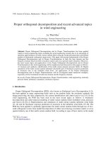
Fig. 39. Dynamic stiffness coefficient, S
24
, obtained by finite-element–boundary-element (the
large dots) and lumped-parameter models with M
= 2( ), M = 6( ), and M = 10
(
).Thethindottedline( ) indicates the weight function w (not in radians), and the
thick dotted line (
) indicates t he high-frequency s olution, i .e. the singular p art of S
24
.
169

Efficient Modelling of Wind Turbine Foundations
56 Will-be-set-by-IN-TECH
0 1 2 3 4 5 6 7 8
0
1
2
3
4
0 1 2 3 4 5 6 7 8
−1
0
1
2
Frequency, f [Hz]
Frequency, f [Hz]
|S
44
| [-]
arg
( S
44
) [rad]
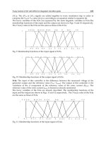
Fig. 40. Dynamic stiffness coefficient, S
44
, obtained by domain-transformation (the large
dots) and l umped-parameter models with M
= 2( ), M = 6( ), and M = 10
(
).Thethindottedline( ) indicates the weight function w (not in radians), and the
thick dotted line (

) indicates t he high-frequency s olution, i .e. the singular p art of S
44
.
6. Summary
This chapter discusses the formulation of computational models that can be used for a n
efficient analysis of wind turbine foundations. The purpose is to allow the introduction of a
foundation model into aero-elastic co des without a dramatic increase in the number of degrees
of freedom in the model. This may be of particular interest for the determination of the fatigue
life of a wind turbine.
After a brief introduction to different types of foundations for wind turbines, the particular
case of a rigid footing on a layered ground is treated. A formulation based on the so-called
domain-transformation method is given, and the dynamic stiffness (or impedance) o f the
foundation is calculated in the frequency domain. The method relies on an analytical solution
for the wave propagation over depth, and this provides a much faster evaluation of the
response to a load on the surface of the ground than m ay be achieved with the finite element
method and other numerical methods. However, the horizontal wavenumber–frequency
domain model is confined t o the analysis of strata with horizontal interfaces.
Subsequently, the concept of a consistent lumped-parameter model (LPM) has been presented.
The basic idea is to adapt a simple mechanical system with few degrees of freedom to the
response of a much more complex system, in this case a wind turbine foundation interacting
with the subsoil. The use of a consistent LPM involves the following steps:
1. The target s olution in the frequency domain is computed by a rigorous m odel, e.g. a
finite-element or boundary-element model. Alternatively the response of a real structure
or footing is measured.
170
Fundamental and Advanced Topics in Wind Power
Efficient Modelling of Wind Turbine Foundations 57
2. A rational filter is fitted to the target results, ensuring that nonphysical resonance is
avoided. The order of the filter should by high enough to provide a good fit, but low
enough to avoid wiggling.

3. Discrete-element models with few internal degrees of freedom are established based on
the rational-filter approximation.
This procedure is carried out for each degree of freedom and the discrete-element models
are then assembled with a finite-element, or similar, model of the structure. Typically,
lumped-parameter models with a three to four internal degrees of freedom provide results of
sufficient accuracy. This has been demonstrated in the present chapter for two different cases,
namely a footing on a stratified ground and a flexible skirted foundation in homogeneous soil.
7. References
Abramowitz, M. & Stegun, I. (1972). Handbook of Mathematical Functions with Formulas,
Graphs and Mathematical Tables, 10 edn, National Bureau of Standards, United States
Department of Commerce.
Achmus, M ., Kuo, Y S. & Abdel-Rahman, K. (2009). Behavior of monopile foundations u nder
cyclic lateral load, Computers and Geotechnics 36(5): 725–735. PT: J; NR: 15; TC: 3; J9:
COMPUT GEOTECH; PG: 11; GA: 447YE; UT: ISI:000266227200005.
Ahmad, S. & Rupani, A. (1999). Horizontal impedance of square foundationsi in layered soil,
Soil Dynamics and Earthquake Engineering 18: 59–69.
Allotey, N. & El Naggar, M . H. (2008). Generalized dynamic winkler model for nonlinear
soil-structure interaction analysis, Canadian Geotechnical Journal 45(4): 560–573. PT: J;
UT: ISI:000255885600008.
Andersen, L . (2002). Wave Propagation in Inifinite Structures and Media, PhD thesis, Department
of Civil Engineering, Aalborg University, Denmark.
Andersen, L. (2010). Assessment of lumped-parameter models for rigid footings, Computers
& S tructures 88: 1333–1347.
Andersen, L. & Clausen, J. (2008). Impedance of s urface f ootings on layered ground, Computers
& S tructures 86: 72–87.
Andersen, L., Ibsen, L. & L iingaard, M. (2009). Lumped-parameter model of a
bucket foundation, in S. Pietruszczak, G. N. Pande, C. Tamagnini & R. Wan
(eds), Computational Geomechanics: COMGEO I, IC2E International Center for
Computational Engineering, pp. 731–742.
API (2000). Recommended practice for planning, designing and constructing fixed offshore

platforms, Rp2a-wsd, American Petroleum Institute, Dallas, Texas, United States of
America.
Asgarian, B., Fiouz, A. & Talarposhti, A. S. (2008). Incremental Dynamic Analysis Considering
Pile-Soil-Structure Interaction for the Jacket Type Offshore Platforms. PT: B; CT: 27th
International Conference on Offshore Mechanics and Arctic Engineering; CY: JUN
15-20, 2008; CL: Estoril, PORTUGAL; U T: ISI:000263876000031.
Auersch, L. (1988). Wechselwirkung starrer und flexibler Strukturen mit dem Baugrund
inbesondere bei Anregnung durch Bodenerschütterungen, BAM-Forschungsbericht
151, Berlin.
171
Efficient Modelling of Wind Turbine Foundations
58 Will-be-set-by-IN-TECH
Auersch, L. (1994). Wave Propagation in Layered Soils: Theoretical Solution in Wavenumber
Domain and Experimental Results of Hammer and Railway Traffic Excitation, Journal
of Sound and Vibration 173(2): 233–264.
Avilés, J. & Pérez-Rocha, L. (1996). A simplified procedure for torsional impedance functions
of embedded foundations in a soil layer, Computers and Geotechnics 19(2): 97–115.
Bathe, K J. (1996). Finite-Element Procedures, 1 edn, John Wiley & Sons Ltd., Chichester.
Brebbia, C. (1982). Boundary Element Methods in Engineering, Springer, Berlin.
Bu, S. & Lin, C. ( 1999). Coupled horizontal–rocking impedance functions for Embedded
Square Foundations at High Frequency Factors, Journal of Earthquake Engineering
3(4): 561–587.
DNV (2001). Foundations, Classification Notes No. 30.4, Det Norske Veritas Classifications A/S,
Høvik, Norway.
Domínguez, J. (1993). Boundary Elements in Dynamics, Computational Mechanics Publications,
Southampton.
El Naggar, M. & Bentley, K. J. (2000). Dynamic analysis for laterally loaded piles and dynamic
p-y curves, Canadian Geotechnical Journal 37(6): 1166–1183. PT : J; NR: 22; TC: 19; J9:
CAN GEOTECH J; PG: 18; GA: 388NU; UT: I SI:000166188300002.
El Naggar, M. & Novak, M. (1994a). Non-linear model for dynamic axial pile response, Journal

of Geotechnical Engineering, ASCE 120(4): 308–329.
El Naggar, M. & Novak, M. (1994b). Nonlinear axial interaction in pile dynamics, Journal of
Geotechnical Engineering, ASCE 120(4): 678–696.
El Naggar, M . & Novak, M. (1995). Nonlinear lateral interaction in pile dynamics, Soil
Dynamics and Earthquake Engineering 14: 141–157.
El Naggar, M. & Novak, M. (1996). Nonlinear analysis for dynamic lateral pile response, Soil
Dynamics and Earthquake Engineering 15: 233–244.
Elleithy, W., Al-Gahtani, H. & El-Gebeily, M. (2001). Iterative coupling of BE and FE method
in e lastostatics, Engineering Analysis with Boudnary Elements 25: 685–695.
Emperador, J. & Domínguez, J. (1989). Dynamic response of axisymmetric embedded
foundations, Earthquake Engineering and Structural Dynamics 18: 1105–1117.
Gerolymos, N. & Gazetas, G. (2006a). Development of wi nkler model for static and dynamic
response of caisson foundations with soil and interface nonlinearities, Soil Dynamics
and Earthquake Engineering 26(5): 363–376. PT: J; NR: 31; TC: 5; J9: SOIL DYNAM
EARTHQUAKE ENG; PG: 14; GA: 032QW; UT: ISI:000236790500003.
Gerolymos, N. & Gazetas, G. (2006b). Static and dynamic response of massive caisson
foundations with soil and interface nonlinearities—validation and results, Soil
Dynamics and Earthquake Engineering 26(5): 377–394. PT: J; NR: 31; TC: 5; J9: SOIL
DYNAM EARTHQUAKE ENG; PG: 14; GA: 032QW; UT: ISI:000236790500003.
Gerolymos, N. & Gazetas, G. (2006c). Winkler model for lateral response of rigid caisson
foundations in linear soil, Soil Dynamics and Earthquake Engineering 26(5): 347–361.
PT: J; NR: 31; TC: 5; J9: SOIL DYNAM EARTHQUAKE ENG; PG: 14; GA: 032QW;
UT: ISI:000236790500003.
Haskell, N. (1953). The Dispersion o f Surface Waves on Multilayered Medium, Bulletin of the
Seismological S ociety of America 73: 17–43.
Houlsby, G. T., Kelly, R. B., Huxtable, J. & Byrne, B. W. (2005). Field trials of suction caissons
in cl ay for offshore wind turbine foundations, Géotechnique 55(4): 287–296.
Houlsby, G. T., Kelly, R. B., Huxtable, J. & Byrne, B. W. (2006). Field trials of suction caissons
in sand for offshore wind turbine foundations, Géotechnique 56(1): 3–10.
172

Fundamental and Advanced Topics in Wind Power
Efficient Modelling of Wind Turbine Foundations 59
Ibsen, L. (2008). Implementation of a new f oundations concept for offshore wind farms,
Proceedings of the 15th Nordic Geotechnical Meeting, Sandefjord, Norway, pp. 19–33.
Jones, C., Thompson, D. & Petyt, M. (1999). TEA — a suite of computer programs for
elastodynamic analysis using coupled boundary elements and finite elements, ISVR
Technical Memorandum 840, Institute of Sound and Vibration Research, University of
Southampton.
Jonkman, J. & Buhl, M. (2005). Fast user’s guide, Technical Report NREL/EL-500-38230, National
Renewable Energy Laboratory, Colorado, United States of America.
Kong, D., Luan, M., Ling, X. & Qiu, Q. (2006). A simplified computational method of
lateral dynamic impedance of single pile considering the effect of separation between
pile and soils, in M. Luan, K. Zen, G. Chen, T. Nian & K. Kasama (eds), Recent
development of geotechnical and geo-environmental engineering in Asia, p . 138. PT: B; CT:
4th Asian Joint Symposium on Geotechnical and Geo-Environmental Engineering
(JS-Dalian 2006); CY: NOV 23- 25, 2006; CL: Dalian, PEOPLES R CHINA; UT:
ISI:000279628900023.
Krenk, S. & Schmidt, H. (1981). Vibration of an Elastic Circular Plate on an Elastic H alf
Space—A Direct Approach, Journal of Applied Mechanics 48: 161–168.
Larsen, T. & Hansen, A. (2004). Aeroelastic effects of large blade deflections for wind turbines,
in D. U. of Technology (ed.), The Science of Making Tor que from Wind, Roskilde,
Denmark, pp. 238–246.
Liingaard, M. (2006). DCE Thesis 3: Dynamic Behaviour of Suction Caissons,PhDthesis,
Department of Civil Engineering, Aalborg University, Denmark.
Liingaard, M., Andersen, L. & Ibsen, L . (2007). Impedance of flexible suction caissons,
Earthquake Engineering and Structural Dynamics 36(13): 2249–2271.
Liingaard, M., Ibsen, L. B. & Andersen, L. (2005). Vertical impedance for stiff and flexible
embedded foundations, 2nd International symposium on Environmental Vibrations:
Prediction, Monitoring, Mitigation and Evaluation (ISEV2005), Okayama, Japan.
Luco, J. (1976). Vibrations of a Rigid Disk on a Layered Viscoelastic Medium, Nuclear

Engineering and Design 36(3): 325–240.
Luco, J. & Westmann, R . (1971). Dynamic Response of Circular Footings, Journal of Engineering
Mechanics, ASCE 97(5): 1381–1395.
Manna, B. & Baidya, D. K. (2010). Dynamic nonlinear response of pile foundations under
vertical vibration-theory versus experiment, Soil Dynamics and Earthquake Engineering
30(6): 456–469. PT: J; UT: ISI:000276257800004.
Mita, A. & Luco, J. (1989). Impedance functions and input motions for embedded square
foundations, Journal of Geotechnical Engineering, ASCE 115(4): 491–503.
Mustoe, G. (1980). A combination of the finite element and boundary integral procedures,PhDthesis,
Swansea University, United Kingdom.
Newmark, N. (1959). A method of computation for structural dynamics, ASCE Journal of the
Engineering Mechanics Division 85(EM3): 67–94.
Novak, M. & Sachs, K. (1973). Torsional and coupled vibrations of embedded footings,
Earthquake Engineering and Structural Dynamics 2: 11–33.
Petyt, M. (1998). Introduction to Finite Element Vibration Analysis, Cambridge: Cambridge
University Press.
Senders, M. (2005). Tripods with suction caissons as foundations for offshore wind turbines on
sand, Proceedings of International Symposium on Frontiers in Offshore Geotechnics: ISFOG
2005, Taylor & Francis Group, London, Perth, Australia.
173
Efficient Modelling of Wind Turbine Foundations
60 Will-be-set-by-IN-TECH
Sheng, X., Jones, C. & Petyt, M. (1999). Ground Vibration Generated by a Harmonic Load
Acting on a Railway Track, Journal of Sound and Vibration 225(1): 3–28.
Stamos, A. & Beskos, D . (1995). Dynamic analysis of large 3-d underground structures b y the
BEM, Earthquake Engineering and Structural Dynamics 24: 917–934.
Thomson, W. (1950). Transmission of Elastic Waves Through a Stratified Solid Medium,
Journal of Applied Physics 21: 89–93.
Varun, Assimaki, D. & Gazetas, G. (2009). A simplified model for lateral response of large
diameter caisson foundations-linear elastic formulation, Soil Dynamics and Earthquake

Engineering 29(2): 268–291. PT: J; NR: 33; TC: 0; J9: SO IL DYNAM EARTHQUAKE
ENG; PG: 24; GA: 389ET; UT: ISI:000262074600006.
Veletsos, A. & Damodaran Nair, V. (1974). Torsional vibration of viscoelastic foundations,
Journal of Geotechnical Engineering Division, ASCE 100: 225–246.
Veletsos, A. & Wei, Y. (1971). Lateral and rocking vibration of footings, Journal of Soil Mechanics
and Foundation Engineering Division, ASCE 97: 1227–1248.
von Estorff, O. & Kausel, E. (1989). Coupling of boundary and finite elements for
soil–structure interaction problems, Earthquake Engineering Structural Dynamics
18: 1065–1075.
Vrettos, C. (1999). Vertical and Rocking Impedances for Rigid Rectangular Foundations
on Soils with Bounded Non-homogeneity, Earthquake Engineering and Structural
Dynamics 28: 1525–1540.
Wolf, J. (1991a). Consistent lumped-parameter models for unbounded soil:
frequency-independent stiffness, damping and mass matrices, Earthquake Engineering
and Structural Dynamics 20: 33–41.
Wolf, J. (1991b). Consistent lumped-parameter models for unbounded soil: p hysical
representation, Earthquake Engineering and Structural Dynamics 20: 11–32.
Wolf, J . ( 1994). Foundation Vibration Analysis Using Simple Physical Models, Prentice-Hall,
Englewood Cliffs, NJ.
Wolf, J. (1997). Spring-dashpot-mass models for foundation vibrations, Earthquake Engineering
and Structural Dynamics 26(9): 931–949.
Wolf, J. & Paronesso, A . (1991). Errata: Consistent lumped-parameter models for unbounded
soil, Earthquake Engineering and Structural Dynamics 20: 597–599.
Wolf, J. & Paronesso, A. (1992). Lumped-parameter model for a rigid cylindrical foundation
in a soil layer on rigid rock, Earthquake Engineering and Structural Dynamics
21: 1021–1038.
Wong, H. & Luco, J. (1985). Tables of impedance functions for square foundations on layered
media, Soil Dynamics and E arthquake Engineering 4(2): 64–81.
Wu, W H. & Lee, W H. (2002). Systematic lumped-parameter models f or foundations based
on p olynomial-fraction approximation, Earthquake Engineering & Structural Dynamics

31(7): 1383–1412.
Wu, W H. & Lee, W H. (2004). Nested lumped-parameter models for foundation vibrations,
Earthquake Engineering & Structural Dynamics 33(9): 1051–1058.
Øye, S. (1996). FLEX4 – simulation of wind turbine dynamics, in B. Pedersen (ed.), State of the
Art of Aeroelastic Codes for Wind Turbine Calculations, Lyngby, Denmark, pp. 71–76.
Yong, Y., Z h ang, R. & Yu, J. (1997). Motion of Foundation on a Layered Soil Medium—I.
Impedance Characteristics, Soil Dynamics and Earthquake Engineering 16: 295–306.
174
Fundamental and Advanced Topics in Wind Power
0
Determination of Rotor Imbalances
Jenny Niebsch
Radon Institute of Computational and Applied Mathematics, Austrian Academy of Sciences
Austria
1. Introduction
During operation, rotor imbalances in wind energy converters (WEC) induce a centrifugal
force, which is harmonic with respect to the rotating frequency and has an absolute value
proportional to the square of the frequency. Imbalance driven forces cause vibrations of the
entire WEC. The amplitude of the vibration also depends on the rotating frequency. If it is
close to the bending eigenfrequency of the WEC, the vibration amplitudes increase and might
even be visible. With the growing size of new WEC, the structure has become more flexible.
As a side effect of this higher flexibility it might be necessary to pass through the critical speed
in order to reach the operating frequency, which leads to strong vibrations. However, even if
the operating frequency is not close to the eigenfrequency, the load from the imbalance still
affects the drive train and might cause damage or early fatigue on other components, e.g., in
the gear unit. This is one possible reason why in most cases the expected problem-free lifetime
of a WEC of 20 years is not achieved. Therefore, reducing vibrations by removing imbalances
is getting more and more attention within the WEC community.
Present methods to detect imbalances are mainly based on the processing of measured
vibration data. In practice, a Condition Monitoring System (CMS) records the development

of the vibration amplitude of the so called 1p vibration, which vibrates at the operating
frequency. It generates an alarm if a pre-defined threshold is exceeded. In (Caselitz &
Giebhardt, 2005), more advanced signal processing methods were developed and a trend
analysis to generate an alarm system was presented. Although signal analysis can detect
the presence of imbalances, the task of identify its position and magnitude remains.
Another critical case arises when different types of imbalances interfere. The two main types
of rotor imbalances are mass and aerodynamic imbalances. A mass imbalance occurs if
the center of gravitation does not coincides with the center of the hub. This can be due to
various factors, e.g., different mass distributions in the blades that can originate in production
inaccuracies, or the inclusion of water in one or more blades. Mass imbalances mainly
cause vibrations in radial direction, i.e., within the rotor plane, but also smaller torsional
vibrations since the rotor has a certain distance from the tower center, acting as a lever for
the centrifugal force. Aerodynamic imbalances reflect different aerodynamic behavior of the
blades. As a consequence the wind attacks each blade with different force and moments.
This also results in vibrations and displacements of the WEC, here mainly in axial and
torsional direction, but also in contributions to radial vibrations. There are multiple causes for
aerodynamic imbalances, e.g., errors in the pitch angles or profile changes of the blades. The
major differences in the impact of mass and aerodynamic imbalances are the main directions
of the induced vibrations and the fact that aerodynamic imbalance loads change with the
7
2 Will-be-set-by-IN-TECH
wind velocity. Nevertheless, if the presence of aerodynamic imbalances is neglected in the
modeling procedure, the determination of the mass imbalance can be faulty, and in the
worst case, balancing with the determined weights can even increase the mass imbalance.
As a consequence, the methods to determine mass imbalance need to ensure the absence of
aerodynamic imbalances first.
In the field, the balancing process of a WEC is done as follows. An on-site expert team
measures the vibrations in the radial, axial and torsion directions. Large axial and torsion
vibrations indicate aerodynamic imbalances. The surfaces of the blades are investigated and
optical methods are used to detect pitch angle deviation. The procedure to determine the

mass imbalance is started after the cause of the aerodynamic imbalance is removed. In this
procedure, the amplitude of the radial vibration is measured at a fixed operational speed,
typically not too far away from the bending eigenfrequency. Afterwards a test mass (usually
a mass belt) is placed at a distinguished blade and the measurements are repeated. From the
reference and the original run, the mass imbalance and its position can be derived. Altogether,
this is a time consuming and personnel-intensive procedure.
In (Ramlau & Niebsch, 2009) a procedure was presented that reconstructed a mass imbalance
from vibration measurements without using test masses. The main idea in this approach
is to replace the reference run by a mathematical model of the WEC. At this stage, only
mass imbalances were considered. A simultaneous investigation of mass and aerodynamic
imbalances was investigated by Borg and Kirchdorf, (Borg & Kirchhoff, 1998). The
contribution of mass and aerodynamic imbalances to the 1p, 2p and 3p vibration was
examined using a perturbation analysis in order to solve the differential equation that coupled
the azimuth and yaw motion. Using the example of an NREL 15 kW turbine, the presence
of 60 % mass imbalance and 40% aerodynamic imbalance explained by a 1 degree pitch
angle deviation was observed. In (Nguyen, 2010) and (Niebsch et al., 2010) the model
based determination of imbalances was expanded to the case of the presence of both mass
imbalances and pitch angle deviation.
The main aim of this chapter is the presentation of a mathematical theory that allows the
determination of mass and aerodynamical imbalances from vibrational measurements only.
This task forms a typical inverse problem, i.e., we want to reconstruct the cause of a measured
observation. In many cases, inverse problems are ill posed, which means that the solution of
the problem does not depend continuously on the measured data, is not unique or does not
exist at all. One consequence of ill-posedness is that small measurement errors might cause
large deviations in the reconstruction. In order to stabilize the reconstruction, regularization
methods have to be used, see Section 3.
Finding the solution of the inverse problem requires a good forward model, i.e., a model that
computes the vibration of the WEC for a given imbalance distribution. This is realized by a
structural model of the WEC, see Section 2. The determination of mass imbalances is briefly
explained in Section 4. The mathematical description of loads from pitch angle deviations is

considered in the same section as well. Section 5 presents the basic principle of the combined
reconstruction of mass and aerodynamic imbalances.
2. Structural model of a wind turbine
2.1 The mathematical model
A structural dynamical model of an object or machine allows to predict the behavior of that
object subjected to dynamic loads. There is a large variety of literature as well as software
addressing this topic. Here, we followed the book (Gasch & Knothe, 1989), where the WEC
176
Fundamental and Advanced Topics in Wind Power
Determination of Rotor Imbalances 3
tower is modeled as a flexible beam, the rotor and nacelle are treated as point masses. The
computation of displacements from dynamic loads can be described by a partial differential
equation (PDE) or an equivalent energy formulation. Usually, both formulations do not result
in an analytical solution. Using Finite Element Methods (FEM), the energy formulation can
be transformed into a system of ordinary differential equations (ODE). The object, in our case
the wind turbine, has to be divided into elements, here beam elements, with nodes at each
end of an element, see Figure 1. The displacement of an arbitrary point of the element is
approximated by a combination of the displacements of the start and the end node. The ODE
system connecting dynamical loads and object displacements has the form
Mu

(t)+Su(t)=p(t). (1)
Here, t denotes the time. The displacements are combined in the vector u, which contains
the degrees of freedom (DOF) of each node in our FE model. The degrees of freedom in
each node can be the displacement
(u, v, w) in all three space directions as well as torsion
around the x-axis and cross sections slopes in the
(x, y) - and (x, z)-plane: (u, v, w, β
x
, β

y
, β
z
),
cf. Figure 2. The physical properties of our object are represented by the mass matrix M and
the stiffness matrix S. The load vector p contains the dynamic load in each node arising from
forces and moments. For this calculation, damping is neglected. Otherwise the term Du

with
damping matrix D adds to the left hand side of equation (1). Considering mass imbalances
Fig. 1. Elements in a Finite Element model of a WEC
only, the forces and moments mainly act in radial direction, i.e., along the z-axis, and result
in displacements and cross section slopes in that direction. Therefore, for each node we only
consider the DOF
(w, β
z
). In order to construct the mass and the stiffness matrix each element
177
Determination of Rotor Imbalances
4 Will-be-set-by-IN-TECH
Fig. 2. Degrees of freedom in a Finite Element model of a WEC
is treated separately. The DOF of the bottom and the top node of the ith element are collected
in the element DOF vector, cf. Figure 2,
u
i
e
=[w
0i
β
z0i

w
i
β
zi
]
T
. (2)
The derivation of the element mass and stiffness matrix M
e
and S
e
uses four shape functions
scaled by the DOF of the bottom and top node to describe the DOF
(w
i
(x), β
zi
(x)) of an
arbitrary point x of the element. It is given in detail in (Gasch & Knothe, 1989). We only
want to present the final formulas for the element matrices,
M
e
=
μL
e
420
⎛
⎜
⎜
⎝

156
−22L
e
54 13L
e
−22L
e
4L
2
e
−13L
e
−3L
2
e
54 −13L
e
156 22L
e
13L
e
−3L
2
e
22L
e
4L
2
e
⎞

⎟
⎟
⎠
, S
e
=
E · I
L
3
e
⎛
⎜
⎜
⎝
12
−6L
e
−12 −6L
e
−6L
e
4L
2
e
6L
e
2L
2
e
−12 6L

e
12 6L
e
−6L
e
2L
2
e
6L
e
4L
2
e
⎞
⎟
⎟
⎠
. (3)
The length of the element is represented by L
e
. E is Young’s modulus, which is a material
constant that can be found in a table . We assume our elements to be circular beam sections.
The transverse moment of inertia I is given by I
= π/64 · (d
4
e,out
−d
4
e,in
) with outer and inner

diameter of the beams section. μ is the translatorial mass per length μ
=  · A, where  is
the density of the material. A
= π/4 · (d
2
e,out
− d
2
e,in
) is the annulus area. To build the full
system matrices S and M, the element matrices S
e
and M
e
are combined by superimposing
the elements affecting the upper node of the ith element matrix with the ones belonging to
the lower node of the
(i + 1)st element matrix, see Figure 3. The sum of rotor mass and
nacelle mass m needs to be added to the last but one diagonal element of the full mass
matrix. As mentioned above, the described model is restricted to radial displacements that
are induced by radial forces, e.g., from mass imbalances. If we consider other types of load,
e.g., aerodynamic, we have to deal with forces and moments in all three space directions. The
derivation of the corresponding mass and stiffness matrix is a bit more comprehensive. In
a general and abbreviated form it is given in (Gasch & Knothe, 1989). The application for a
WEC is presented in Niebsch et al. (2010), and in a more detailed version in (Nguyen, 2010).
178
Fundamental and Advanced Topics in Wind Power
Determination of Rotor Imbalances 5
1
2

3
4
Fig. 3. System matrix and superimposed element matrices
2.2 Model optimization
Once M and S are determined, the solution of equation (1) for a given load p provides the
displacement of each node in our model. We remark that the FEM is an approximative
method. Additionally, the idealization of WEC as a flexible beam with a point mass as well as
slight deviations in the geometric and physical parameters lead to model that approximates
the reality but can not reproduce it exactly. Hence the system properties of our model,
described by M and S, might differ slightly from the properties of the real WEC. In order
to calibrate the model to the real WEC we have to chose one or more parameters that can be
measured at the real WEC and then optimize our model according to those parameters. For
our application the most important parameter of a WEC is the first (bending) eigenfrequency
of the system. For each WEC type a range for the first eigenfrequency is given by the
manufacturer, e.g., a VESTAS V80 of 100 m height has an eigenfrequency in the range
[0.21, ···, 0.255]Hz. The actual eigenfrequency of a specific WEC of any type depends, e.g.,
on the grounding of the WEC and manufacturing tolerances in geometry and material. The
eigenfrequency can be obtained from measurements during the performance of an emergency
stop of the WEC. Thus our model, i.e., the matrices M and S, derived for a certain type of
WEC from given geometrical and physical parameters as described above, can be optimized
for specific WECs of that type with respect to the measured first eigenfrequency. The first
eigenfrequency of the model can be computed using the assumption u
(t)=u
0
exp(λt) and
inserting it in the homogenous form of (1). Then we have to solve
λ
2
Iu
0

= −M
−1
Su
0
, (4)
i.e., λ
2
are the eigenvalues of the matrix −M
−1
S. For example, they can be obtained with the
Matlab function eig. The eigenvalues are complex numbers. In the absence of damping, as in
our case, the real part vanishes. The eigenfrequencies ω
ei g
are given by the imaginary part:
ω
ei g
= ±


−eig(M
−1
S)

. (5)
The rotational first eigenfrequency is then given by
Ω
0
=
min{ω
ei g

}
2π
. (6)
179
Determination of Rotor Imbalances
6 Will-be-set-by-IN-TECH
Usually there is no information of the foundation and grounding available whereas
manufacturing tolerances in the geometry, i.e., the length and the inner and outer diameter
of the beam elements are accessible in the modeling process. In fact, Ω
0
is a function of those
parameters. We can chose the geometric parameters from realistic intervals of manufacturing
tolerances in such a way that the new model eigenfrequency is very close to the measured
one. Supposing Ω is the measured first eigenfrequency of the WEC, the optimal geometric
parameters can be found by minimizing the functional
min
L,d
in
,d
out
|Ω − Ω
0
(L, d
in
, d
out
)|, (7)
where the vectors L, d
in
, d

out
contain the length, inner and outer diameter of each element.
3. Introduction to inverse problems
Within this Section, we would like to introduce some basic concepts from the theory of inverse
and ill posed problems. We will focus in particular on regularization theory, which has been
extensively developed over the last decades. As we will see, regularization is always needed
when the solution of a problem does not depend continuously on the data, which causes in
particular problems if the data originate from (noisy) measurements. For details, we refer to
(Engl et al., 2000).
We assume that the connection of two terms f and g such as an imbalance and the
displacements resulting from that imbalance, is described by an operator A:
A f
= g. (8)
The computation of g for given f is called the forward problem while the determination of f
for given g is referred to as the inverse problem. In practical applications the exact data g are
not known but a measured noisy version g
δ
of that data. We assume that the noise level is
bounded by an unknown number δ, i.e.,
g − g
δ
≤δ. (9)
The computation of an imbalance from vibration/displacement data is an inverse problem.
If the following three conditions are fulfilled, the Inverse Problem is called well posed:
1. For all data g there exists a solution f .
2. The solution f is unique.
3. The solution f depends continuously on the data g.(A
−1
is continuous.)
The last condition ensures that small changes in the data g result in small changes in the

solution f. A well posed inverse problem can be solved by applying the inverse operator to
the data:
f
= A
−1
g. (10)
If one of the conditions is violated the inverse problem is called ill posed.
The violation of condition 1 can be fixed by the definition of a generalized solution. We
compute our solution as the least-squares solution taking f as the element that minimizes
the distance of A f to the data g:
f
†
= arg min
f
A f − g
2
. (11)
180
Fundamental and Advanced Topics in Wind Power
Determination of Rotor Imbalances 7
The operator that maps the data g to the least-squares solution f
†
is denoted by A
†
and called
generalized inverse of A. The violation of condition 2 can be rectified by distinguishing one
solution from the set of all solutions. It can be the solution with the smallest norm or the one
that best fits prior known properties of the desired solution.
In condition 3 we have to deal with the discontinuous inverse or generalized inverse operator.
Small errors in the data can result in huge errors in the solution. To avoid this behavior, the

discontinuous inverse is approximated pointwise by a family of continuous operators. To
be more precise, we have to find a family of operators T
α
, with a regularization parameter
α
= α(δ, g
δ
), that fulfills the conditions
α
(δ)
δ→0
−−→ 0, lim
δ→0
T
α
g
δ
= A
†
g. (12)
This implies that for very small data error δ the parameter α becomes small and the
corresponding continuous T
α
is a good approximation to A
†
. The right choice of α is difficult
because the error we get by computing f
δ
α
= T

α
g
δ
as an approximate solution of f
†
= A
†
g
has two parts that behave very differently:
T
α
g
δ
−A
†
g≤ T
α
g
δ
−T
α
g
  
pro p ag ated data error
+ T
α
g −A
†
g
  

appro x i m a tio n error
. (13)
The approximation error decreases with α while the propagated data error increases with
decreasing α, cf. Figure 4. This is due to the fact that for small α the operator T
α
is closer to
A
†
and thus ”less continuous” than for bigger α. The total error has a minimum away from
α
= 0. To find the parameter α with minimal error T
α
g
δ
− A
†
g, a parameter choice rule is
necessary. The operator family defined in (12) combined with a parameter choice rule is called
regularization method.
A widely used example for a regularization method is Tikhonov’s regularization where the
operator T
α
is given by
T
α
=(A
∗
A + αI)
−1
A

∗
, (14)
where I is the identity and A
∗
denotes the adjoint operator of A. In case A is a matrix, A
∗
is
the transpose of A. Alternatively, f
δ
α
= T
α
g
δ
can be characterized as the unique minimizer of
the Tikhonov functional
J
α
( f )=A f − g
δ

2
+ αf 
2
. (15)
The characterization of f
δ
α
via the Tikhonov functional is in particular important as it allows
a straightforward generalization for nonlinear operators. The linear operator can simply be

replaced by a nonlinear operator. We mention this because the consideration of aerodynamic
imbalances leads to a nonlinear operator A. The determination of the regularization
parameter α depends on properties of the operator and the choice of the regularization
method, (Engl et al., 2000). In principle, there are a-priori parameter choice rules, where α
can be determined from prior information, and a-posteriori rules. A well known a posteriori
parameter choice rule is Morozov’s discrepancy principle where α is chosen s.t.
δ
≤g
δ
−A f
δ
α

2
≤ cδ (16)
holds (Morozov, 1984). The application of the discrepancy principle requires the computation
of the approximate solution f
δ
α
for a chosen α first. Afterwards (16) is checked and α has to be
181
Determination of Rotor Imbalances
8 Will-be-set-by-IN-TECH
Fig. 4. Regularization error
changed if the condition does not hold. All a-posteriori parameter choice rules depend on the
data error level δ and the data g
δ
. Very popular are heuristic parameter choice rules, where
the regularization parameter is independent of the noise level δ. Examples are the L-curve
method (Hansen P., 1992) or the quasi-optimality rule (Kindermann, 2008). Please note that

heuristic parameter choice rules do not lead to convergent regularization methods, although
they perform well in many applications.
4. Imbalance determination
The determination of imbalances from measurements of the induced vibrations (or
displacements) is an inverse problem as explained above.
4.1 Mass imbalance
First, we restrict ourself to the determination of mass imbalances and assume that
aerodynamic imbalances are insignificant. In the structural model section we mentioned that
in this case we only need a model that considers DOF in radial or z-direction. The knowledge
of the mass and stiffness matrix provides us with a connection of the loads from imbalances p
and the resulting displacements u in the nodes of our model via equation (1).
A mass imbalance can be described by a mass m that is located at a distance r from the rotor
center and has an angle ϕ to a certain zero mark of the rotor, usually blade A, cf. Figure 5. If
the rotor revolves with revolutionary frequency Ω, the mass imbalance induces a centrifugal
force of absolute value ω
2
mr, with the angular velocity ω = 2πΩ. The force or load vector is
given by:
p
(t)=ω
2
mre
i(ωt+ϕ)
=: p
0
ω
2
e
iωt
, (17)

where p
0
= mre
iϕ
defines the mass imbalance in absolute value and phase location. Harmonic
loads of the form (17) cause harmonic vibration u
= u
0
e
iωt
of the same frequency ω. Inserting
u, its second derivative and p
= p
0
e
iωt
into equation (1), time dependency cancels out and
we get an explicit solution for the vibration amplitudes u
0
:
u
0
=(−M + ω
−2
S)
−1
p
0
. (18)
182

Fundamental and Advanced Topics in Wind Power
Determination of Rotor Imbalances 9
Radius r
Phase
angle
φ
m
A
B
C
Fig. 5. Mass imbalance
The matrix
(−M + ω
−2
S)
−1
would define our forward operator in (8 ) if we would assume
that the vibration amplitudes could be measured in every node of the model. Usually this is
not possible, measurements are taken in the nacelle which is represented by the last model
node, cf. Figure 1. Additionally, the rotor and its load are located at that node, too. Thus
the load vector p
0
would have only one entry, p
0
from (17), at the last but one position that
corresponds to the displacement DOF w of the last node. Hence in (8) now f
= p
0
, g = u
0

the
displacement of the last node, and A is just the element in the last but one row and last but
one column of
(−M + ω
−2
S)
−1
. Denoting the number of DOF by N we have
Ap
0
= u
0
, A =(−M + ω
−2
S)
−1
(N−1,N−1)
. (19)
We remark that u
0
is the complex amplitude containing the absolute value and the phase angle
u
0
= u
a
e
iφ
.
The measured values for u
a

and φ are denoted by u
δ
a
and φ
δ
. Since A is a complex number we
deal with the simplest well posed inverse problem possible. It is solved by
p
δ
0
=
1
A
u
δ
0
. (20)
4.2 Aerodynamic imbalance from pitch angle deviation
The main cause for aerodynamic imbalances is a deviation between the pitch angles of the
blades, e.g., from assembling inaccuracies. Depending on the wind conditions, even a small
deviation of one of the pitch angles can cause large forces and moments to be transferred onto
the rotor. This results in displacements in direction of the rotor axis (the y-axis) as well as
torsion around the tower axis (x-axis). But there are also forces in radial direction that add
to the forces from mass imbalances and are not negligible. Hence, neglecting aerodynamic
imbalances could result in an inaccurate determination of mass imbalances. In the worst
case, the computed balancing mass and position could increase the mass imbalance. The
mass imbalance estimation described in the former section can only be applied if aerodynamic
imbalances are small enough. Currently, the WEC is checked for axial and torsional vibrations.
If large corresponding amplitudes indicate an aerodynamic imbalance, the surfaces of the
blades are checked and photographic measurements are carried out to find a possible pitch

183
Determination of Rotor Imbalances
10 Will-be-set-by-IN-TECH
angle deviation. After its correction the mass imbalance can be determined with the usual
method.
The simultaneous reconstruction of mass and aerodynamic imbalances was considered in
(Nguyen, 2010) and (Niebsch et al., 2010). The principle is the same as in the reconstruction of
mass imbalances but now the structural model of the WEC is extended to DOF in radial and
axial direction as well as torsion around the tower axis. Additionally, we have to describe
the loads from aerodynamic imbalances mathematically. This was done using the Blade
Element Momentum (BEM) theory, which is commonly used for simulations of WECs, see,
e.g., (Hansen, 2008; Ingram, 2005). The result of the BEM theory are the tangential and normal
(or thrust) force distributed over the blades that are divided into elements. The distributed
forces are summed up to an equivalent normal force F
i
with a distance l
i
from the rotor center
as well as an equivalent tangential force T
i
, cf. Figure 6.
(a) Thrust forces F
i
(b) Tangential forces T
i
Fig. 6. Normal (thrust) and tangential forces on the rotor blades
The forces depend on the pitch angle of the blade, the airfoil data, the angle of attack of the
wind, and the relative wind velocity, as well as a lift and drag coefficient table. For details we
refer to (Niebsch et al., 2010).
The force to the rotor in the axial (y-) direction is calculated by:

F
y
= F
1
+ F
2
+ F
3
. (21)
The moments induced by this forces are given by
M
1
x
= F
1
l
1
sin(ωt + φ)+F
2
l
2
sin(ωt + φ + ϕ)+F
3
l
3
sin(ωt + φ + 2ϕ),
M
1
z
= F

1
l
1
cos(ωt + φ)+F
2
l
2
cos(ωt + φ + ϕ)+F
3
l
3
cos(ωt + φ + 2ϕ), (22)
where M
1
x
and M
1
z
denote the moments around the x- and the z-axis on the rotor and ϕ =
2π
3
(≡ 120
◦
) is the angle between the rotor blades. Note that if all blades have the same pitch
angle, we have F
1
= F
2
= F
3

and l
1
= l
2
= l
3
. This means that the moments M
1
x
and M
1
z
vanish. The projection of the total tangential force T = T
1
+ T
2
+ T
3
onto the z-axis and the
x-axis is given by
T
z
= T
1
cos(ωt + φ)+T
2
cos(ωt + φ + ϕ)+T
3
cos(ωt + φ + 2ϕ), (23)
T

x
= T
1
sin(ωt + φ)+T
2
sin(ωt + φ + ϕ)+T
3
sin(ωt + φ + 2ϕ).
184
Fundamental and Advanced Topics in Wind Power
Determination of Rotor Imbalances 11
Since we have a small distance D between rotor plane and the tower center, T
z
and T
x
also
produce moments around the x- and the z-axes:
M
2
x
= T
z
· D, M
2
z
= T
x
· D. (24)
With the formulas (21) - (24) we can describe the load vector p
(t) in (1), which has only entries

at the last node. We recall that the node has the DOF
(v, w, β
x
, β
y
, β
z
), hence
p
=(0, ···,0,F
y
, F
z
, M
x
, M
y
, M
z
)
T
, (25)
with F
z
= T
z
, M
x
= M
1

x
+ M
2
x
, and M
z
= M
1
z
+ M
2
z
. We remark that M
y
is converted into the
rotational movement and finally into electrical energy. M
y
should not add any contribution
to the load vector.
5. Combination of mass and aerodynamic imbalances
The simultaneous consideration of mass and aerodynamic imbalances is also based on
equation (1). As mentioned in the last section, for aerodynamic imbalances a model is required
that includes DOF in the radial and axial directions as well as torsion around the tower axis.
The combined presence of both imbalance types also requires a combination of the associated
load vectors. We recall that the centrifugal force from a point mass imbalance is given by
ω
2
mr, the location of the eccentric mass is given by the radius r and the angle φ
m
measured

from a zero mark (blade A). The projections of the force onto the z- and x-axis are
F
2
z
= ω
2
mr cos(ωt + φ + φ
m
), (26)
F
x
= ω
2
mr sin(ωt + φ + φ
m
).
Here, φ is the angle between blade A and the x-axis. Because the rotational plane has a
distance D to the tower, the forces F
2
z
and F
x
also produce moments around the x- and the
z-axes:
M
3
x
= F
2
z

· D, (27)
M
3
z
= F
x
· D.
The force in x-direction is of no consequence since we assume the tower to be rigid. But the
moments M
3
x
, M
3
z
and the force F
2
z
have to be added to the moments and forces from pitch
angle deviation as described in (25). The forces and moments of the combined load vector
add to
F
y
= F
1
+ F
2
+ F
3
F
z

= T
z
+ F
2
z
(28)
M
x
= M
1
x
+ M
2
x
+ M
3
x
M
z
= M
1
z
+ M
2
z
+ M
3
z
.
We observe that the forces and moments in (28) are either constant (F

y
) or harmonic. Therefore,
equation (1) with a load vector of the form (25) and entries (28) can be solved explicitly. Details
on the solution are given in (Niebsch et al., 2010).
Starting from the pitch angles of the three blades
(θ
1
, θ
2
, θ
3
), and from the characteristics of
a mass imbalance
(mr , φ
m
) and assuming given values for angular speed ω = 2πΩ, wind
185
Determination of Rotor Imbalances
12 Will-be-set-by-IN-TECH
speed, and airfoil data, we have all the tools to determine the corresponding imbalance load p
using the BEM method for the pitch angle deviation and by projecting (17) onto the x- and the
z-axis. Solving (1) produces the resulting displacements u. The restriction of the vector u onto
the DOF that can be measures are denoted by g
= u
|sensor
. We combine all these operations
into the forward operator A:
A
(θ
1

, θ
2
, θ
3
, mr, φ
m
)=g. (29)
We remark that the BEM uses nonlinear optimization routines to compute parameter values
in the equations for the normal and tangential force. Therefore, the final operator A is
nonlinear. The vector
(θ
1
, θ
2
, θ
3
, mr, φ
m
) plays the role of f in (8). Usually, the radial
and axial vibration, and the torsion around the tower axis are measurable using three
acceleration sensors. Since the acceleration sensors do not measure the initial offset arising
from the constant force F
y
we have to rely on radial and torsion measurements only. For
a known or estimated noise level δ of the measurements we can compute the solution
(θ
1
, θ
2
, θ

3
, mr, φ
m
)
δ
α
as the minimizer of the Tikhonov functional (15). Since A is a nonlinear
operator, minimization methods have to be employed to find the minimizing element, like
e.g., the MATLAb implemented routines like fminsearch or gradient based methods. The
regularization parameter α can be chosen iteratively using Morozov’s Discrepancy Principle
(16). First results on the simultaneous reconstruction of
(θ
1
, θ
2
, θ
3
, mr, φ
m
) from noisy data g
δ
were obtained in (Niebsch et al., 2010) with data errors of about 10%. Several experiments
showed that the simultaneous reconstruction is successful provided we have a fairly good
initial value for the mass imbalance. This can be obtained in a first step by reconstructing
the mass imbalance neglecting pitch angle deviations with the method described in Section
4. The result is not the true mass imbalance but a sufficiently accurate initial estimate for
the simultaneous reconstruction carried out as a second step. To present an example, a pitch
angle deviation of 3 degree of the blade B as well as a mass imbalance of 350 kgm located at
blade B. The data g were calculated by the forward computation of A
(0

◦
,3
◦
,0
◦
, 350 kgm, 120
◦
)
and contaminated with 10% noise. The two step reconstruction from the noisy data resulted
in
(−0.25
◦
, 2.8
◦
, 0.43
◦
, 342 kgm, 121
◦
). The correction of the pitch angles and the setting
of balancing weights according to that reconstruction lead to a significant reduction of the
vibration, cf. Figure 7.
Fig. 7. Vibrations in z-direction before and after balancing
186
Fundamental and Advanced Topics in Wind Power
Determination of Rotor Imbalances 13
6. Conclusion
We presented a method to determine imbalances from vibration measurements based on a
relatively simple model of the WEC under consideration. In contrast to detection methods
based on signal processing, the imbalance can be localized and quantified. Moreover, mass
imbalances and pitch angle deviations that cause aerodynamic imbalances can be discovered

simultaneously. The model of the WEC is used to describe the connection of an imbalance
load and the caused vibrations or displacements mathematically. The reverse direction of
recovering an imbalance from given noisy vibration measurements is an inverse (ill-posed)
problem and has to be treated accordingly. For this reason, we presented a short introduction
to the main ideas and issues of the inverse problem theory.
In addition to the model parameters, the presented method requires the mathematical
description of the loads from the different types of imbalances. Whereas for mass imbalances
this is quite simple, the forces from pitch angle deviation are computed via the BEM method
which uses idealizations that do not cover all effects that might arise during the operation
of the WEC. Another drawback of the determination of pitch angle deviations is the fact
that the BEM method requires the airfoil data of the WEC’s blades. For most of the newer
wind turbines this data are a well kept secret of the manufacturers. The restriction of
the imbalance estimation to mass imbalances is much easier to implement into an existing
condition monitoring system and does not require "sensitive" data.
We propose two main questions for future research. First, the assumption of a constant
revolution frequency is not realistic. Therefore we have to consider equation (1) for a variable
(time dependent) angular velocity ω, which allows the use of vibration data measured at
variable speed. Presently, only data collected with constant or almost constant operational
speed can be used for the imbalance determination. The second question is how to avoid the
sensitive information on airfoil data that is necessary to reconstruct pitch angle deviations.
7. References
Borg, J. P. & Kirchhoff, R. H. (1998). Mass and Aerodynamic Imbalance of a Horizontal Axis
Wind Turbine. ASME Journal of Solar Energy Engineering Vol. 120, 66-74.
Ciang, C. C., Lee, J., Bang, H. (2008). Structural health monitoring for a wind turbine system:
a review of damage detection methods. Meas.Sci.Technol. , Vol. 19,122001(20pp).
Caselitz, P. & Giebhardt, J. (2005). Rotor Condition Monitoring for Improved Operational
Safety of Offshore Wind Energy Converters. ASME Journal of Solar Energy Engineering
Vol. 127, 253-261.
Engl, H. W ; Hanke, M. & Neubauer, A. (2000). Regularization of Inverse Problems, Kluwer,
Dortrecht.

Gasch, R. & Knothe, K. (1989). Strukturdynamik 2, Springer, Berlin.
Hau, E. (2006). Wind Turbines: Fundamentals, Technologies, Application, Economics; Springer,
Berlin, Heidelberg.
Hansen, M. (2008). Aerodynamics of Wind Turbines; Earthscan, London.
Hansen, P. C. (1992). Analysis of discrete ill-posed problems by means of the L-curve. SIAM
Rev; Vol. 34 561-580.
Ingram, G. (2005). Wind Turbine Blade Analysis using the Blade Element Momentum Method.
Note on the BEM method, Durham University, Durham.
187
Determination of Rotor Imbalances
14 Will-be-set-by-IN-TECH
Kindermann, S. & Neubauer, A. (2008) On the convergence of the quasi-optimality criterion
for (iterated) Tikhonov regularization. Inverse Problems and Imaging Vol. 2, Nr. 2,
291-299.
Morozov, V. A. (1984). Methods for Solving Incorrectly posed Problems, Springer, New York, Berlin
Heidelberg.
Niebsch, J.; Ramlau, R. & Nguyen, T. T. (2010). Mass and aerodynamic Imbalance Estimates of
Wind Turbines. Engergies, Vol. 3, p 696-710, ISSN 1996-1073.
Nguyen, T. T. (2010). Mass and aerodynamic Imbalance Estimates of Wind Turbines. Diploma
thesis at the Johannes Kepler University Linz, Austria.
Ramlau, R. (2002). Morozov’s Discrepancy Principle for Tikhonov regularization of nonlinear
operators. Numerical Functional Analysis and Optimization, Vol. 23 No.1&2, 147-172.
Ramlau, R. & Niebsch, J. (2009). Imbalance Estimation Without Test Masses for Wind Turbines.
ASME Journal of Solar Energy Engineering Vol. 131, No. 1, 011010-1- 011010-7.
Scherzer, O. (1993). Morozov’s Discrepancy Principle for Tikhonov regularization of nonlinear
operators. Computing, Vol. 51 , 45-60.
188
Fundamental and Advanced Topics in Wind Power
8
Wind Turbine Gearbox Technologies

Adam M. Ragheb
1
and Magdi Ragheb
2
1
Department of Aerospace Engineering
2
Department of Nuclear, Plasma and Radiological Engineering,
University of Illinois at Urbana-Champaign, 216 Talbot Laboratory
USA
1. Introduction
The reliability issues associated with transmission or gearbox-equipped wind turbines and
the existing solutions of using direct-drive (gearless) and torque splitting transmissions in
wind turbines designs, are discussed. Accordingly, a range of applicability of the different
design gearbox design options as a function of the rated power of a wind turbine is
identified. As the rated power increases, it appears that the torque splitting and gearless
design options become the favored options, compared with the conventional, Continuously
Variable Transmission (CVT), and Magnetic Bearing transmissions which would continue
being as viable options for the lower power rated wind turbines range.
The history of gearbox problems and their relevant statistics are reviewed, as well as the
equations relating the gearing ratios, the number of generator poles, and the high speed and
low speed shafts rotational speeds.
Aside from direct-drive systems, the topics of torque splitting, magnetic bearings and their
gas and wind turbine applications, and Continuously Variable Transmissions (CVTs), are
discussed.
Operational experience reveals that the gearboxes of modern electrical utility wind turbines
at the MegaWatt (MW) level of rated power are their weakest-link-in-the-chain component.
Small wind turbines at the kW level of rated power do not need the use of gearboxes since
their rotors rotate at a speed that is significantly larger than the utility level turbines and can
be directly coupled to their electrical generators.

Wind gusts and turbulence lead to misalignment of the drive train and a gradual failure of
the gear components. This failure interval creates a significant increase in the capital and
operating costs and downtime of a turbine, while greatly reducing its profitability and
reliability. Existing gearboxes are a spinoff from marine technology used in shipbuilding
and locomotive technology. The gearboxes are massive components as shown in Fig. 1.
The typical design lifetime of a utility wind turbine is 20 years, but the gearboxes, which
convert the rotor blades rotational speed of between 5 and 22 revolutions per minute (rpm)
to the generator-required rotational speed of around 1,000 to 1,600 rpm, are observed to
commonly fail within an operational period of 5 years, and require replacement. That 20
year lifetime goal is itself a reduction from the earlier 30 year lifetime design goal (Ragheb &
Ragheb, 2010).

Fundamental and Advanced Topics in Wind Power
190
2. Gearbox issues background
The insurance companies have displayed scrutiny in insuring wind power generation. The
insurers joined the rapidly-growing market in the 1990s before the durability and long term
maintenance requirements of wind turbines were fully identified. To meet the demand, a
number of units were placed into service with limited operational testing of prototypes.
During the period of quick introduction rate, failures during wind turbines operation were
common. These included rotor blades shedding fragments, short circuits, cracked foundations,
and gearbox failure. Before a set of internationally recognized wind turbine gearbox design
standards was created, a significant underestimation of the operational loads and inherent
gearbox design deficiencies resulted in unreliable wind turbine gearboxes.
The lack of full accounting of the critical design loads, the non-linearity or unpredictability
of the transfer of loads between the drive train and its mounting fixture, and the
mismatched reliability of individual gearbox components are all factors that were identified


Fig. 1. Top view of a Liberty Quantum Drive 2.5 MW rated power wind turbine gearbox

(Source: Clipper Windpower).

Wind Turbine Gearbox Technologies
191
by the National Renewable Energy Laboratory (NREL) as contributing to the reduced
operating life of gearboxes (Musial et al., 2007).
In 2006, the German Allianz reportedly received 1,000 wind turbine damage claims. An
operator had to expect damage to his facility at a 4-5 years interval, excluding malfunctions
and uninsured breakdowns.
As a result of these earlier failures, insurers adopted provisions that require the inclusion by
the operator of maintenance requirements into their insurance contracts. One of the
common maintenance requirements is to replace the gearbox every 5 years over the 20-year
design lifetime of the wind turbine. This is a costly task, since the replacement of a gearbox
accounts for about 10 percent of the construction and installation cost of the wind turbine,
and will negatively affect the estimated income from a wind turbine (Kaiser &
Fröhlingsdorf, 2007). Figure 1 depicts the size of the Quantum Drive gearbox of a Liberty
2.5 MW wind turbine (Clipper Windpower, 2010)
The failure of wind turbine gearboxes may be traced to the random gusting nature of the
wind. Even the smallest gust of wind will create an uneven loading on the rotor blades,
which will generate a torque on the rotor shaft that will unevenly load the bearings and
misalign the teeth of the gears. This misalignment of the gears results in uneven wear on
the teeth, which in turn will facilitate further misalignment, which will cause more uneven
wear, and so on in a positive feedback way.
The machine chassis will move, which will misalign the gearbox with the generator shaft
and may eventually cause a failure in the high speed rear gearing portion of the gearbox.
Further compounding the problem of uneven rotor blade loading is the gust slicing effect,
which refers to multiple blades repeatedly traveling through a localized gust (Burton et al.,
2004). If a gust of wind were to require 12 seconds to travel through the swept area of a
wind turbine rotor operating at 15 rpm, each of the three blades would be subject to the gust
three times, resulting in the gearbox being subjected to a total of nine uneven loadings in a

rapid succession.
The majority of gearboxes at the 1.5 MW rated power range of wind turbines use a one- or
two-stage planetary gearing system, sometimes referred to as an epicyclic gearing system.
In this arrangement, multiple outer gears, planets, revolve around a single center gear, the
sun. In order to achieve a change in the rpm, an outer ring or annulus is required.







Fig. 2. Planetary gearing system.
Sun,
g
enerator shaft



Annulus, rotor shaft

Planet


Fundamental and Advanced Topics in Wind Power
192
As it would relate to a wind turbine, the annulus in Fig. 2 would be connected to the rotor
hub, while the sun gear would be connected to the generator. In practice however, modern
gearboxes are much more complicated than that of Fig. 2, and Fig. 3 depicts two different
General Electric (GE) wind turbine gearboxes.

Fig. 3. GE 1P 2.3 one-stage planetary and two-stage parallel shaft (top) and 2P 2.9 two-stage
planetary and one-stage parallel shaft (bottom) wind turbine gearboxes (Image: GE).

Wind Turbine Gearbox Technologies
193
Planetary gearing systems exhibit higher power densities than parallel axis gears, and are able
to offer a multitude of gearing options, and a large change in rpm within a small volume. The
disadvantages of planetary gearing systems include the need for highly-complex designs, the
general inaccessibility of vital components, and high loads on the shaft bearings. It is the last
of these three that has proven the most troublesome in wind turbine applications.
In order to calculate the reduction potential of a planetary gear system, the first step is to
determine the number of teeth, N, that each of the three component gears has. These values
will be referred to as:
,,
sun annulus
p
lanet
NN andN

as they relate to the number of teeth on the sun, annulus, and planet gears, respectively.
Using the relationship that the number of teeth is directly proportional to the diameter of a
gear, the three values should satisfy Eqn. 1, which shows that the sun and annulus gears
will fit within the annulus.

2
sun

p
lanet annulus
NN N


(1)
With Eqn. 1 satisfied, the equation of motion for the three gears is,
2210
sun sun sun
annulus sun planet
planet planet planet
NN N
NN N
 
 

  
 
 
(2)
where: ω
sun
, ω
annulus
, and ω
planet
are the angular velocities of the respective gears.
Since the angular velocity and is directly proportional to the revolutions per minute (rpm),
Eqn. 2 may be modified to Eqn. 3 below.

2210
sun sun sun
annulus sun planet
planet planet planet
NN N
rpm rpm rpm
NN N
 
 

 
 
 
(3)
Known values may be substituted into Eqn. 3 in order to determine the relative rpm values
of the sun and annulus gears, noting the two equalities of Eqns. 4 and 5 below (Ragheb &
Ragheb, 2010).

sun
sun
p
lanet
planet
N
rpm rpm
N






(4)

planet
p
lanet annulus
annulus
N
rpm rpm
N





(5)
Historically, the gearbox has been the weakest link in a modern, utility scale wind turbine.
Following the current trend of larger wind turbines for offshore applications with their
larger rotor diameters and heavier rotor blades, gearboxes are being subject to significantly
increased loads.
Minor improvements in the gearbox lubrication and oil filtration system have increased the
reliability of wind turbines, but to significantly improve the gearbox reliability, the design