Fundamental and Advanced Topics in Wind Power Part 10 ppt

The Analysis and Modelling of a Self-excited
Induction Generator Driven by a Variable Speed Wind Turbine
259
I =
















;V
cq
=







|

0 ; V
cq
=







|
0
Any combination of R, L and C can be added in parallel with the self-excitation capacitance
to act as load. For example, if resistance R is added in parallel with the self-excitation
capacitance, then the term 1/pC in (equation 20) becomes R/(1+RpC). The load can be
connected across the capacitors, once the voltage reaches a steady-state value (Grantham et
al., 1989), (Seyoum et al., 2003).
The type of load connected to the SEIG is a real concern for voltage regulation. In general,
large resistive and inductive loads can vary the terminal voltage over a wide range. For
example, the effect of an inductive load in parallel with the excitation capacitor will reduce
the resulting effective load impedance (Z
eff
) (Simoes & Farret, 2004).
Z
eff
= R + j


 (26)
This change in the effective self-excitation increases the slope of the straight line of the

capacitive reactance (Figure 3), reducing the terminal voltage. This phenomenon is more
pronounced when the load becomes highly inductive.
5. Simulation results
A model based on the first order differential equation (equation 25) has been built in the
MATLAB/Simulink to observe the behavior of the self-excited induction generator. The
parameters used, obtained from (Krause et al., 1994), are as follows.

Machine Rating IB
(abc) r
r
r
s
X
|
s X
|
r Xm J
Hp Volts Rpm Amps Ohms Ohms Ohms Ohms Ohms
Kg.m
^

500 2300 1773 93.6 0.187 0.262 1.206 1.206 54.02 11.06
Table 1. Induction Machine Parameters
All the above mentioned values are referred to the stator side of the induction machine and
the value of self-exciting capacitance used is 90 micro farads.
From the previous subsection, it can be said that with inductive loads the value of excitation
capacitance value should be increased to satisfy the reactive power requirements of the SEIG
as well as the load. This can be achieved by connecting a bank of capacitors, across the load
meeting its reactive power requirements thereby, presenting unity power factor
characteristics to the SEIG. It is assumed in this thesis that, such a reactive compensation is

provided to the inductive load, and the SEIG always operates with unity power factor.
5.1 Saturation curve
As explained in the previous section, the magnetizing inductance is the main factor for
voltage build up and stabilization of generated voltage for theunloaded and loaded
conditions of the induction generator (Figure 3). Reference (Simoes & Farret, 2004) presents
a method to determine the magnetizing inductance curve from lab tests performed on a
machine. The saturation curve used for the simulation purposes is, obtained from (Wildi,

Fundamental and Advanced Topics in Wind Power
260
1997) by making use of the B-H saturation curve of the magnetic material (silicon iron 1%),
shown in Figure 9.


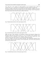
Fig. 9. Variation of magnetizing inductance with magnetizing current.
Using least square curve fit, the magnetizing inductance Lm can be expressed as a function
of the magnetizing current I
m
as follows:
L
m
= 1.1*(0.025+0.2974*exp(-0.00271*I
m
)) (27)
Where,
I
m
=

















It must be emphasized that the machine needs residual magnetism so that the self-excitation
process can be started. Reference (Simoes & Farret, 2004) gives different methods to recover
the residual magnetism in case it is lost completely. For numerical integration, the residual
magnetism cannot be zero at the beginning; its role fades away as soon as the first iterative
step for solving (equation 25) has started.
5.2 Process of self-excitation
The process of self-excitation can be compared with the resonance phenomenon in an RLC
circuit whose transient solution is of the exponential form Ke
p
1t
(Elder et al., 1984),
(Grantham et al., 1989). In the solution, K is a constant, and root p
1
is a complex quantity,
whose real part represents the rate at which the transient decays, and the imaginary part is
proportional to the frequency of oscillation. In real circuits, the real part of p

1
is negative,
meaning that the transient vanishes with time. With the real part of p
1
positive, the transient
(voltage) build-up continues until it reaches a stable value with saturation of iron circuit. In
other terms, the effect of this saturation is to modify the magnetization reactance X
m
, such
that the real part of the root p
1
becomes zero in which case the response is sinusoidal steady-
state corresponding to continuous self-excitation of SEIG.
Any current (resulting from the voltage) flowing in a circuit dissipates power in the circuit
resistance, and an increasing current dissipates increasing power, which implies some
energy source is available to supply the power. The energy source, referred to above is
provided by the kinetic energy of the rotor (Grantham et al., 1989).
With time varying loads, new steady-state value of the voltage is determined by the self-
excitation capacitance value, rotor speed and load. These values should be such that they
The Analysis and Modelling of a Self-excited
Induction Generator Driven by a Variable Speed Wind Turbine
261
guarantee an intersection of magnetization curve and the capacitor reactance line (Figure 3),
which becomes the new operating point.
The following figures show the process of self-excitation in an induction machine under no-
load condition.


Fig. 10. Voltage build up in a self-excited induction generator.
From Figures 10 and 11, it can be observed that the phase voltage slowly starts building up

and reaches a steady-state value as the magnetization current I
m
starts from zero and reaches
a steady-state value. The value of magnetization current is calculated from the
instantaneous values of stator and rotor components of currents (see (equation 27)). The
magnetization current influences the value of magnetization inductance Lm as per (3.27),
and also capacitance reactance line (Figure 3). From Figures 10-12, we can say that the self-
excitation follows the process of magnetic saturation of the core, and a stable output is
reached only when the machine core is saturated.
In physical terms the self-excitation process could also be explained in the following way.
The residual magnetism in the core induces a voltage across the self-exciting capacitor that
produces a capacitive current (a delayed current). This current produces an increased
voltage that in turn produces an increased value of capacitor current. This procedure goes
on until the saturation of the magnetic filed occurs as observed in the simulation results
shown in Figures 10 and 11.


Fig. 11. Variation of magnetizing current with voltage buildup.

Fundamental and Advanced Topics in Wind Power
262

Fig. 12. Variation of magnetizing inductance with voltage buildup.
For the following simulation results the WECS consisting of the SEIG and the wind turbine
is driven by wind with velocity of 6 m/s, at no-load. At this wind velocity it can only supply
a load of approximately 15 kW. At t=10 seconds a 200 kW load is applied on the WECS. This
excess loading of the self-excited induction generator causes the loss of excitation as shown
in the Figure 13.

Fig. 13. Failed excitation due to heavy load.


Fig. 14. Generator speed (For failed excitation case)
The Analysis and Modelling of a Self-excited
Induction Generator Driven by a Variable Speed Wind Turbine
263
Figure 14 shows the rotor speed variations with load during the loss of excitation. The
increase in load current should be compensated either by increasing the energy input (drive
torque) thereby increasing the rotor speed or by an increase in the reactive power to the
generator. None of these conditions were met here which resulted in the loss of excitation. It
should also be noted from the previous section that there exists a minimum limit for speed
(about 1300 rpm for the simulated machine with the self-excitation capacitance equal to 90
micro-farads), below which the SEIG fails to excite.
In a SEIG when load resistance is too small (drawing high load currents), the self-excitation
capacitor discharges more quickly, taking the generator to the de-excitation process. This is
a natural protection against high currents and short circuits.
For the simulation results shown below, the SEIG-wind turbine combination is driven with
an initial wind velocity of 11m/s at no-load, and load was applied on the machine at t=10
seconds. At t = 15 seconds there was a step input change in the wind velocity reaching a
final value of 14 m/s. In both cases the load reference (full load) remained at 370 kW. The
simulation results obtained for these operating conditions are as follows:


Fig. 15. SEIG phase voltage variations with load.
For the voltage waveform shown in Figure 15, the machine reaches a steady-state voltage of
about 2200 volts around 5 seconds at no-load. When load is applied at t=10seconds, there is
a drop in the stator phase voltage and rotational speed of the rotor (shown in Figure 18) for
the following reasons.
We know that the voltage and frequency are dependent on load (Seyoum et al., 2003).

Loading decreases the magnetizing current I
m
, as seen in Figure 16, which results in the
reduced flux. Reduced flux implies reduced voltage (Figure 15). The new steady-state values
of voltage is determined (Figure 3.3) by intersection of magnetization curve and the
capacitor reactance line. While the magnitude of the capacitor reactance line (in Figure 3) is
influenced by the magnitude of I
m
, slope of the line is determined by angular frequency
which varies proportional to rotor speed. If the rotor speed decreases then the slope
increases, and the new intersection point will be lower to the earlier one, resulting in the
reduced stator voltage. Therefore, it can be said that the voltage variation is proportional to
the rotor speed variation (Figure 18). The variation of magnetizing current and magnetizing
inductance are shown in the Figures 16 and 17 respectively.

Fundamental and Advanced Topics in Wind Power
264
Magnetization current, Im

Time (seconds)
Fig. 16. Magnetizing current variations with load.


Fig. 17. Magnetizing inductance variations with load.
Figures 16 and 17 verify that the voltage is a function of the magnetizing current, and as a
result the magnetizing inductance (see (equation 27)), which determines the steady-state
value of the stator voltage.


Fig. 18. Rotor speed variations with load

Figure 18, shows the variations of the rotor speed for different wind and load conditions.
For the same wind speed, as load increases, the frequency and correspondingly
synchronous speed of the machine decrease. As a result the rotor speed of the generator,
which is slightly above the synchronous speed, also decreases to produce the required
amount of slip at each operating point.
The Analysis and Modelling of a Self-excited
Induction Generator Driven by a Variable Speed Wind Turbine
265
As the wind velocity increases from 11m/s to 14m/s, the mechanical input from the wind
turbine increases. This results in the increased rotor speed causing an increase in the stator
phase voltage, as faster turning rotor produces higher values of stator voltage. The
following figures show the corresponding changes in the SEIG currents, WECS torque and
power outputs.


Fig. 19. Stator current variations with load.


Fig. 20. Load current variations with load.
From Figures 19 and 20, we see that as load increases, the load current increases. When the
machine is operating at no-load, the load current is zero. When the load is applied on the
machine, the load current reaches a steady-state value of 100 amperes (peak amplitude).
With an increase in the prime mover power input, the load current further increases and
reaches the maximum peak amplitude of 130 amperes. Also, the stator and load currents
will increase with an increase in the value of excitation capacitance. Care should be taken to
keep these currents with in the rated limits. Notice that, in the case of motor operation stator
windings carry the phasor sum of the rotor current and the magnetizing current. In the case
of generator operation the machine stator windings carry current equal to the phasor
difference of the rotor current and the magnetizing current. So, the maximum power that
can be extracted as a generator is more than 100% of the motor rating (Chathurvedi &

Murthy, 1989).

Fundamental and Advanced Topics in Wind Power
266

Fig. 21. Variation of torques with load.


Fig. 22. Output power produced by wind turbine and SEIG.
Equation 17, has been simulated to calculate the electromagnetic torque generated in the
induction generator. Figure 21 also shows the electromagnetic torque T
e
and the drive
torque Tdrive produced by the wind turbine at different wind speeds. At t=0, a small drive
torque has been applied on the induction generator to avoid simulation errors in Simulink.
Figure 22 shows the electric power output of the SEIG and mechanical power output of the
wind turbine. The electric power output of the SEIG (driven by the wind turbine), after t=10
seconds after a short transient because of sudden increase in the load current (Figure 20), is
about 210 kW at 11 m/s and reaches the rated maximum power (370 kW) at 14 m/s. Pitch
controller limits (see chapter 1) the wind turbine output power, for wind speeds above 13.5
m/s, to the maximum rated power. This places a limit on the power output of the SEIG also,
preventing damage to the WECS. Since, the pitch controller has an inertia associated with
the wind turbine rotor blades, at the instant t=15seconds the wind turbine output power
sees a sudden rise in its value before pitch controller starts rotating the wind turbine blades
out of the wind thereby reducing the value of rotor power coefficient. Note that the power
loss in the SEIG is given by the difference between P
out
and Pwind, shown in Figure 22.
6. Conclusion
In this chapter the electrical generation part of the wind energy conversion system has been

presented. Modeling and analysis of the induction generator, the electrical generator used in
The Analysis and Modelling of a Self-excited
Induction Generator Driven by a Variable Speed Wind Turbine
267
this chapter, was explained in detail using dq-axis theory. The effects of excitation capacitor
and magnetization inductance on the induction generator, when operating as a stand-alone
generator, were explained. From the simulation results presented, it can be said that the self-
excited induction generator (SEIG) is inherently capable of operating at variable speeds. The
induction generator can be made to handle almost any type of load, provided that the loads
are compensated to present unity power factor characteristics. SEIG as the electrical
generator is an ideal choice for isolated variable-wind power generation schemes, as it has
several advantages over conventional synchronous machine.
7. References
Al Jabri A. K. and Alolah A. I, (1990) “Capacitance requirements for isolated self-excited
induction generator,” Proceedings, IEE, pt. B, vol. 137, no. 3, pp. 154-159
Basset E. D and Potter F. M. (1935), “Capacitive excitation of induction generators,” Trans.
Amer. Inst. Elect. Eng, vol. 54, no.5, pp. 540-545
Bimal K. Bose (2003), Modern Power Electronics and Ac Drives, Pearson Education, ch. 2
Chan T. F., (1993) “Capacitance requirements of self-excited induction generators,” IEEE
Trans. Energy Conversion, vol. 8, no. 2, pp. 304-311
Dawit Seyoum, Colin Grantham and M. F. Rahman (2003), “The dynamic characteristics of
an isolated self-excited induction generator driven by a wind turbine,” IEEE
Trans. Industry Applications, vol.39, no. 4, pp.936-944
Elder J. M, Boys J. T and Woodward J. L, (1984) “Self-excited induction machine as a small
low-cost generator,” Proceedings, IEE, pt. C, vol. 131, no. 2, pp. 33-41
Godoy Simoes M. and Felix A. Farret, (2004) Renewable Energy Systems-Design and Analysis
with Induction Generators, CRC Press, 2004, ch. 3-6
Grantham C., Sutanto D. and Mismail B., (1989) “Steady-state and transient analysis of self-
excited induction generators,” Proceedings, IEE, pt. B, vol. 136, no. 2, pp. 61-68
Malik N. H. and Al-Bahrani A. H., (1990)“Influence of the terminal capacitor on the

performance characterstics of a self-excited induction generator,” Proceedings, IEE,
pt. C, vol. 137, no. 2, pp. 168-173
Mukund. R. Patel (1999), Wind Power Systems, CRC Press, ch. 6
Murthy S. S, Malik O. P. and Tandon A. K., (1982)“Analysis of self excited induction
generators,” Proceedings, IEE, pt. C, vol. 129, no. 6, pp. 260-265
Ouazene L. and Mcpherson G. Jr, (1983) “Analysis of the isolated induction generator,” IEEE
Trans. Power Apparatus and Systems, vol. PAS-102, no. 8, pp.2793-2798
Paul.C.Krause, Oleg Wasynczuk & Scott D. Sudhoff (1994), Analysis of Electric Machinery,
IEEE Press, ch. 3-4
Rajesh Chathurvedi and S. S. Murthy, (1989) “Use of conventional induction motor as a
wind driven self-excited induction generator for autonomous applications,” in
IEEE-24
th
Intersociety Energy Conversion Eng. Conf., IECEC, pp.2051-2055
Salama M. H. and Holmes P. G., (1996) “Transient and steady-state load performance of
stand alone self-excited induction generator,” Proceedings, IEE-Elect. Power Applicat.,
vol. 143, no. 1, pp. 50-58
Sreedhar Reddy G. (2005), Modeling and Power Management of a Hybrid Wind-Microturbine
Power Generation System, Masters thesis., ch. 3

Fundamental and Advanced Topics in Wind Power
268
Theodore Wildi, (1997) Electrical Machines, Drives, and Power Systems, Prentice Hall, Third
Edition, pp. 28
Wagner C. F, (1939) “Self-excitation of induction motors,” Trans. Amer. Inst. Elect. Eng, vol.
58, pp. 47-51
12
Optimisation of the Association of
Electric Generator and Static Converter
for a Medium Power Wind Turbine

Daniel Matt
1
, Philippe Enrici
1
, Florian Dumas
1
and Julien Jac
2

1
Institut d’Electronique du Sud, Université Montpellier 2
2
Société ERNEO SAS
France
1. Introduction

This chapter shows the ways of optimising a medium power wind power electromechanical
system, generating anything up to several tens of kilowatt electric power. The optimisation
criteria are based on the cost of the electromechanical generator associated with a power
electronic converter; on the power efficiency; and also on a fundamental parameter, often
neglected in smaller installations, which is torque ripple. This can cause severe noise pollution.
For a wind turbine generating several kW of electric power, the best solution, without a
shadow of a doubt, is to use a permanent magnet electromagnetic generator. This type of
generator has obvious advantages in terms of reliability, ease of operation and above all,
efficiency. Despite problems concerning the cost of magnets, almost all manufacturers of
small or medium power wind turbines use permanent magnet generators (Gergaud et al.
2001). This chapter deals with this type of system. The objective is to demonstrate that only a
judicious choice of the configuration of the permanent magnet synchronous generator,
amongst the different options, will allow us to satisfy the criteria required for optimal
performance. We will study examples of a conventional permanent magnet generator with

distributed windings, a permanent magnet generator with concentrated windings
(Magnusson & Sandrangani, 2003) and a non-conventional Vernier machine (Matt & Enrici,
2005). How these different machines work will be detailed in the following paragraphs.
2. Description of the electromechanical conversion system
The chosen electromechanical conversion system is represented in Fig. 1. The principle of a
turbine directly driving a generator has been chosen in preference to adding a speed
multiplier gearbox between the turbine and the generator.
There are many advantages to using a mechanical drive without a gearbox, which requires
regular maintenance and which has a pronounced rate of breakdown. These devices are also
a significant source of noise pollution when sited near housing. Noise pollution is one of the
principal factors in the chosen optimisation criteria. Finally, the gearbox can cause chemical
pollution due to the lubricant which it contains. However, the omission of a gearbox means
an increase in both size and cost of the generator, which then operates at a very low speed.

Fundamental and Advanced Topics in Wind Power

270
For this reason, a balance between size, cost and performance of the system must be
considered. More and more wind turbine manufacturers are using the direct drive concept.


Fig. 1. Structure of the conversion system
As stated, one of the major design difficulties is sizing the generator, which whilst operating
at low speed, must supply high torque. The size is proportional to the torque so the mass or
volume power ratio of a generator tends to be low.
The main deciding parameter for the size of the generator is the electrical conversion
frequency. These energy systems are therefore all sized on the same basis: the frequency of
the completed conversion cycle (electric, thermal, mechanical). The optimal solution chosen
for the generator will have the characteristics of a "high frequency" machine, typically
between 100 and 200 Hz or even more in certain cases, for a rotation speed generally in the

order of 100 to 200 rpm. In this context, optimised direct drive gives a mass-power ratio
close to that obtained by an indirect drive, with increased efficiency and reliability. This
quest for high conversion frequencies is beneficial to noise pollution, high frequency
vibrations being more easily filtered by the mechanical structure of the wind turbine.
A second design difficulty concerns the choice of static converter associated with the
machine, in order to fulfil the generating requirements of the end user. This is a difficult
choice, because the behaviour of the converter can have serious repercussions on the
behaviour of the generator with regard to the chosen performance criteria.
Whether the turbine is on an isolated site or is connected to the grid, most power electronic
converters have a DC bus like that in Fig. 1. The study presented in this chapter will be
limited mainly to DC bus systems i.e. combined with a permanent magnet synchronous
generator and rectifier.
It should be noted that direct AC to AC conversion solutions, like that in Fig. 2, adapted for
linking the generator to the grid, exist (Barakati, 2008), but while these solutions are appealing
on paper, they haven’t really been put into practice. They conflict with the design of the matrix
converter which uses bidirectional switches for coupling (Thyristor solutions also exist).
We return to diagram on Fig. 1 which corresponds to the system under study. Different
solutions exist for the rectifier. They are shown in Fig. 3.
Two of these are based on the concept of active rectifiers. The structure of these rectifiers is
that of an inverted PWM inverter, the energy flowing from an AC connection to a DC
connection (Mirecki, 2005; Kharitonov, 2010). A variation of this structure, called Vienna,
also uses the notion of a bidirectional switch (Kolar et al, 1998).
The interest of an active rectifier lies in the fact that the driver gives complete control of the
current waveform produced by the generator, the rectifier itself imposes no specific stress on

Optimisation of the Association
of Electric Generator and Static Converter for a Medium Power Wind Turbine

271

Fig. 2. Connection of generator to the grid using a matrix converter


Fig. 3. Different configurations of rectifiers
the machine. If the EMF of the generator is sinusoidal, control of the rectifier will give a
sinusoidal current in phase with the EMF, the ohmic loss will be minimised, the sizing
optimal. This configuration and ideal operating mode will serve as a reference in the
following paragraphs for comparing different generator configurations.
The disadvantage of using active rectifiers is essentially economic. The structure of the
power electronic used, although classic, is complex, which makes for high costs and poor
reliability, especially in comparison with the solutions which we are soon going to present.
In the case of medium power, which is the focus of this chapter, the active rectifier, despite
its drawbacks, is the most common solution.
Despite the undeniable advantages of active rectifiers, the conventional structure of passive
diode rectifiers can be preferable in wind turbine systems because they are robust in most
conditions. These are the two other solutions illustrated in Fig. 3. The rectifier can be used
alone, or with a chopper when a degree of fine tuning is required in maintaining optimal
performance of the system. The chopper is not always indispensable and only slightly
improves the performance of the wind turbine. (Gergaud, 2001; Mirecki, 2005).
We will confine ourselves therefore to the study of a permanent magnet synchronous
generator with a passive diode rectifier. We will show that by careful selection of the
configuration of the generator, highly satisfactory operation of the conversion system is

Fundamental and Advanced Topics in Wind Power

272
achieved, with minimal drop in performance (efficiency, torque ripple) compared to a
system using an active rectifier.
3. Choosing the structure of the synchronous generator
To satisfy the conditions which we have imposed, we will study the behaviour of three

distinct permanent magnet synchronous generators: a conventional structure widely used; a
"Vernier" structure (Toba & Lipo, 2000; Matt & Enrici, 2005), less well known, but perfectly
adapted to operating at very low speed; and a harmonic coupling structure (Magnussen &
Sadarangani, 2003), nowadays a classic, but little used in the field of wind turbines. Their
operating modes are reviewed in the following paragraphs. The conventional structure will
serve as a reference by which to compare the other two structures, which are better adapted
to running at high frequencies for low rotation speeds.
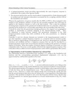
The electrical system under study will be modelled on the diagram in Fig. 4. The electrical
generator is represented by a simplified Behn-Eschenburg model, which is sufficiently
precise for this general comparison. This model is particularly pertinent, since the 3
machines studied generate sinusoidal EMF with almost no harmonics.
The addition of the "DC model" gives an accurate estimation of the reduction in average
rectified voltage, E
s
, due on the one hand to the overlap engendered by the synchronous
inductance, Ls, of the generator (
Ee
), and on the other hand to resistive voltage drop, (
Er
),
(Mirecki, 2005). This demonstrates the power limitation associated with synchronous
inductance. Thus, conforming to the rules of impedance matching, the maximum power,
P
max
, transferred to the continuous load is obtained when E
b
= E
s
/2, which allows us to
express the following:

P
max
=

2
4
s
E
YR
(1)


Fig. 4. Modelling of the Electrical System
This phenomenon of power limitation can be used to advantage in a wind turbine with a
passive conversion system, without regulating power. It is then possible, with the
appropriate value of parameter Y (see Table 1), to obtain close to maximum power (MPPT),
at variable speed, without any control mechanism (Matt et al.; 2008). However, the
optimisation of the inductance L
s
on which Y depends, will be dictated by the compromises
reached, which we will explain in the descriptions of the studied generators (Abdelli, 2007).
The following table shows the main notations used for the study of the electrical system.
Optimisation of the Association
of Electric Generator and Static Converter for a Medium Power Wind Turbine

273
Electrical parameters Notations

Remarks
Electric frequency, pulsation

f
e
, 
-
Rotation speed, pulsation of rotation
N, 
r

-
Coefficient of torque or EMF k
T
In steady state
Phase EMF E In steady state
Synchronous inductance L
s
In steady state
Phase resistor r In steady state
Number of pole pair p -
Filtering inductance L
1
Optional
DC bus voltage E
b
-
Average rectified voltage E
s
3 phases Graetz rectifier
Overlap "resistor" Y Non dissipative
DC model resistor R Dissipative
Table 1. Variables of the electrical system

The comparative study of the following three generators was done using a CAD power
electronics tool (PSIM, Powersim Inc.), based on the diagrams in Figs. 1 and 4.
The three structures compared are of a similar cylindrical design and overall size. They are
designed to supply an electrical output of 10 KW for a rotation speed of 150 rpm.
4. Operation using a conventional synchronous generator
The first permanent magnet generator studied is a classic design. Its general structure is
represented in Fig. 5. The armature of this machine has a three-phase pole pitch winding
with a large number of poles of which we will list the precise characteristics. The field
system magnets are fixed along the rotor rim and form an almost continuous layer.


Fig. 5. Conventional Permanent magnet generator
Rather than designing a generator specifically for this comparison, we have chosen to adopt
the characteristics of a commercial machine, currently used in medium power wind

Fundamental and Advanced Topics in Wind Power

274
turbines. The useful characteristics for the model are summed up in Table 2 (refer to Table 1
for the notations).

Characteristics Values
Nominal rotation speed (rpm) 150
f
e
at nominal speed (Hz) 45
Nominal power with resistive load (W) 9740
E at nominal rotation speed (steady state) (V) 160
r (steady state) ()
1

L
s
(mH) 7,4
p 18
Joule losses at nominal current (W) 1600
Iron and mechanical losses (W) 200
Torque ripple without load (cogging torque) (Nm) 8
Nominal efficiency with resistive load (%) 84
Table 2. Characteristics of the reference generator
The principal characteristic of this generator lies in the angle of the slots which greatly
reduce cogging torque ripple (8 Nm). Another consequence of this angle is the limitation of
the harmonics of the electromotive forces which, as a result, are practically sinusoidal.
The optimisation of the mass-power ratio of this machine is achieved by using as many
poles as possible in order to obtain a high electrical operating frequency. The winding,
however, cannot have more than 36 poles because of the high number of slots (108). The
working frequency is therefore equal to 45 Hz at the speed of 150 rpm. This phenomenon is
a major structural drawback for conventional low speed designs.
This generator is sold as a kit, only the active parts are supplied. The stator comprises the
armature, magnetic circuit and windings, inside an aluminium tube; the rotor is made up of
a steel tube to which are attached the magnets. The dimensions are shown in Table 3.

Dimensions Values
External diameter (mm) 500
Airgap diameter (mm) 400
Stator length (mm) 175
Rotor length (mm) 110
Internal diameter of the rotor (mm) 350
Mass, rotor and stator (kg) 73
Table 3. Principal dimensions of a conventional generator
The electrical parameters in Table 2 are given for operation with the armature giving

directly onto a resistive load. The power factor is then unitary but the current is slightly out
of phase in relation to the electromotive force (dephasing of an angle   20°).
Operating with an active rectifier as mentioned in paragraph 2 allows minimisation of the
armature current for any given power due to the phasing of the current with the
Optimisation of the Association
of Electric Generator and Static Converter for a Medium Power Wind Turbine

275
electromotive force. This ideal mode of operation will give us a reference efficiency of 10 kW
at 150 rpm. With sinusoidal current, the electromotive force being sinusoidal, torque ripple
is negligible; only cogging torque remains, measured at 8 Nm by the manufacturer.
Simulated study of this operating mode is pointless, given the simplicity of the waveforms
produced through the use of this rectifier.
With the data in Table 2 we get the following characteristics:

Characteristics Values
Output power (kW) 10
EMF, E (V) 160
Armature RMS current (A) 20,8
Joule losses (W) 1300
Iron and mechanical losses (W) 200
Efficiency (%) 87
Torque ripple (%) 1
Table 4. Operating in cos = 1 (active rectifier)
The slight gain in efficiency obtained here, as we have already mentioned, is at the cost of an
increase in complexity of the conversion system.
We are now going to study the consequences of operating with a strictly passive rectifier,
which we recommend for this kind of application.
Digital simulation of the above gives the following waveforms for armature current (set
against the electromotive force) and the electromagnetic power.

Fig. 6. Waveforms with passive rectifier
Table 5 shows the results obtained.
The deterioration of the current form engendered by the rectifier has two important
consequences. In the first place, the appearance of harmonics and the dephasing of the
current with the EMF leads to a significant increase in the RMS value of the current for any
given power, the output passes from 87% with an active rectifier to 76% with a diode
rectifier. There is significant derating of the generator. Secondly, the current harmonics
increase significantly the rate of torque ripple which goes from a value of almost zero to


Fundamental and Advanced Topics in Wind Power

276
Characteristics Values
Output power (kW) 10
EMF, E (V) 160
Armature RMS current (A) 31,5
Joule losses (W) 2976
Iron and mechanical losses (W) 200
Efficiency (%) 76
Torque ripple (%) 13
Table 5. Operating with a diode rectifier
close to 13%. This phenomenon is far from being insignificant: it causes operating noise, one
of the main disadvantages of wind turbines.
Torque ripple produces a resonant frequency that is audible and unpleasant, often close to
the natural frequency of the structure. In our example, this frequency is equal to six times
the first harmonic frequency, i.e. 270 Hz.
Medium power wind turbines are often situated near to residential areas so this torque ripple

problem can be very disturbing. An effective way of remedying the problem would be to
augment the parameter L
s
of the generator, but this would reduce efficiency even further.
Therefore, the type of generator presented does not work well with a passive rectifier.
The result presented is obtained with a voltage source load, E
b
. This is possible thanks to the
synchronous inductance of the generator which smooths out the output current. Further
filtering, through the inductance L
1
, is often added, if only to limit ripple current load when
E
b
is an accumulator, or to smooth out the output voltage in the case of a load on a
capacitive bus.
The waveforms obtained with an inductance L
1
of 20mH are shown in Fig. 7.


Fig. 7. Waveforms with a passive rectifier and filter choke
The introduction of a filter choke L
1
, has the notorious consequence of increasing the rate of
electromechanical power ripple, which is precisely what we wish to reduce, as shown in the
results in Table 6.
From here on, we will no longer factor in the inductance L
1
which is detrimental to operation.

Optimisation of the Association
of Electric Generator and Static Converter for a Medium Power Wind Turbine

277
Characteristics Values
Output power (kW) 10
EMF, E (V) 160
Armature current (RMS) (A) 32,7
Joule losses (W) 3207
Iron and mechanical losses (W) 200
Efficiency (%) 75
Torque ripple (%) 21
Table 6. Operating with diode rectifier and filter choke
To recap, two intrinsic characteristics of the conventional structure of a generator limit
performance in a passive rectifier configuration: the operating frequency, which is difficult
to increase because of the way the armature is designed, and ohmic loss which remains high
for this application.
5. Operation of a Vernier permanent magnet synchronous generator
The Vernier synchronous generator, using magnets, is an interesting and viable alternative
to the last configuration. Despite being the subject of numerous studies (Toba & Lipo, 2000;
Matt & Enrici, 2005; Matt et al, 2007) it is less well known. It is represented in Fig. 8.


Fig. 8. Vernier permanent magnet synchronous generator
The design of the Vernier generator is similar to the example previously studied ( Fig 5), but
with the Vernier machine the component used in the magnetic field results from the
coupling between the field system magnets and variation of reluctance due to the armature
slots. Operation is modified as follows.
The armature of the Vernier machine has exactly the same structure as a conventional
machine, the polyphase winding with p pole pairs spread out through the N

s
slots which are
wide open.

Fundamental and Advanced Topics in Wind Power

278
The structure of the field system is also similar to that of a conventional machine, but the
number of pairs of magnets, N
r
, along the rotor rim is not at all related to the number of
pole-pairs: it can be much larger. This is what makes the Vernier generator unique. The
working electrical frequency of the machine is now uniquely linked to N
r
, as seen in the
following formula:

r
.T
e
=
2
r
N

 f
e
=
1
e

T
=
.
2
rr
N



(2)
This frequency can be high, even though the number of pole-pairs may be small. The
limitations on frequency increase at low rotation speeds are generally lower than for the
preceding configuration.
In closing this descriptive summary, we can summarise the coupling relations between the
magnetic fields, expressed in terms of the only spatial variable, , which is the azimuthal
coordinate in the airgap.
The N
s
slots airgap permeance has a periodicity equal to 2/Ns. The airgap magnetomotive
force created by the magnets, having a remanent flux density equal to M, has a periodicity
equal to 2/Nr. Consequently, the field component, b
1an
, created by the magnets, and
having the periodicity 2/|Ns-Nr|, comes into play. This can be expressed thus:
b
1an
= k
1
.M.cos((N
s

-N
r
).)

(3)
The coefficient k
1
, which defines the field amplitude b
1an
(), is deduced using the finite
elements method (of an elementary domain) (Matt, & Enrici, 2005), as in Fig. 9. It’s value,
which depends on the ratios of the dimensional proportion parameters, is generally between
0,1 et 0,2. This is not the most precise of methods since the slot pitch is slightly different
from the magnet pitch, but in most cases it is sufficiently accurate.


Fig. 9. Magnet-slot interaction in the elementary domain
The flux density field component, b
1an
, is the main component used in the Vernier machine.
The armature currents can be likened to a thin coating (Matt et al, 2011) of current,
conventionally called electric loading, 
1
, with a periodicity equal to 2/p, which we will
express thus:

1
= A
1
.cos(p)

(4)
The amplitude, A
1
, of the electric loading, is obtained by looking at the ratio of the amount
of current at the core of the slot and that at the slot pitch, taking into account the winding
factor.
Optimisation of the Association
of Electric Generator and Static Converter for a Medium Power Wind Turbine

279
The magnetic field, b
1an
, and the magnetomotive force created by the electric loading, 
1
,
combine to generate electromagnetic torque, C
em
, provided that the spatial periodicity of
b
1an
and 
1
are identical. The following formula must therefore be verified:
|Ns-Nr| = p

(5)
Once this first condition is met, and the functions (3) and (4) are in phase, the
electromagnetic torque will be maximised.
The formula (4) shows that the number of pole-pairs, p, is dissociated from the number of

magnet pairs, N
r
, since the choice of number of slots is relatively large.
For the electromechanical conversion to take place, it is necessary to verify a second
condition: the rotation speeds of b
1an
and the magnetomotive force produced by 
1
must be
identical, which, taking into account the spatial periodicity of the two functions, leads to the
following expression:


rr rr
sr
NN
p
p
NN





= 
c
(6)
The expression (6) obtained being identical to the expression (2), the main criteria for
optimal operation are met.
The formula (7) above demonstrates the ratio of the field speed, 

c
, to the rotor speed, 
r
:

cr
v
r
N
K
p




(7)
The coefficient K
v
, the speed ratio, is called the Vernier Ratio, and is characteristic of the
eponymous machine.
We shall conclude this explanatory part by expressing the electromagnetic torque, C
em
, of
the Vernier machine, which refers to the principal elements that we have just cited:
C
em
= K
v
.R².L.
11

2

an
bd





(8)
The dimensions R and L of the expression (8) represent the airgap radius and the iron length
respectively. This expression can be misleading: the coefficient K
v
seems to be a torque-
multiplying coefficient if we refer to traditional expressions, whereas here, this coefficient
compensates the low flux density b
1an
(see (3)).
In practice, direct comparison of the performance levels of the Vernier configuration and
that of a conventional configuration is delicate (Matt & Enrici, 2005). We simply note here
that increasing the operating frequency, which the design of the Vernier machine allows,
gives a gain of 50 to 100% in the mass-power ratio at very low speed, at the price of a
substantial increase in rotor manufacturing costs.
The Fig. 10 shows an example of industrial production for a small electric car with a Vernier
engine.
Unfortunately, at present, there is no commercialised Vernier generator specific to the field
of wind turbines. We will therefore base our comparison on a theoretically scaled model.
The sizing calculations are not within the scope of the summary that we are presenting and
will not be detailed, but the references given in the prior explanations cover the main
elements.

Fundamental and Advanced Topics in Wind Power

280
For this theoretical sizing, we will use a maximum number of the characteristics of the
preceding generator in order to ensure the most precise comparison, notably when
discussing the thermic aspects, which are always difficult to comprehend in a scaled model.
The size is similar (even the external dimensions), and the configuration of the armature
winding will be identical (same number of slots, same number of poles).



Fig. 10. Vernier engine for an electric vehicle (photography ERNEO)
Unfortunately, at present, there is no commercialised Vernier generator specific to the field of
wind turbines. We will therefore base our comparison on a theoretically scaled model. The
sizing calculations are not within the scope of the summary that we are presenting and will not
be detailed, but the references given in the prior explanations cover the main elements.
For this theoretical sizing, we will use a maximum number of the characteristics of the
preceding generator in order to ensure the most precise comparison, notably when
discussing the thermic aspects, which are always difficult to comprehend in a scaled model.
The size is similar (even the external dimensions), and the configuration of the armature
winding will be identical (same number of slots, same number of poles).
The following table presents the principal characteristics obtained with a Vernier generator
operating in association with an active rectifier.
The main dimensions of this generator are shown in Table 8.
The advantages of this configuration in the context of wind turbines, which impose an
operating point with high torque for a very low speed of rotation, are shown in the folowing
two tables.
Given that the mode of interaction between the magnets and slots results in a continuous
and gradual shift of the magnets relative to the slots, which increases as the numbers N

s
and
N
r
increase, the Vernier structure is a machine of naturally sinusoidal electromotive force
with almost zero cogging torque and no slot tilt.
We observe that the high operating frequency at low speed, 225 Hz instead of 45 Hz, leads
to a mass-power ratio of more than two times that obtained previously. We go from
140 W/kg to around 380 W/kg (without the housing) taking into account only the weight of
the active parts.
Finally, the efficiency of the sized Vernier machine is comparable to a conventional machine,
in the same operating conditions, with three times more iron loss, but with half the Joule

Optimisation of the Association
of Electric Generator and Static Converter for a Medium Power Wind Turbine

281
Characteristics Values
N
s
/ N
r
108 / 90
Number of pole-pairs, armature winding 18
Nominal rotation speed (rpm) 150
f
e
at nominal rotation speed (Hz) 225
Output power (kW) 10
E at nominal rotation speed (steady state) (V) 166

r (steady state) ()
0,44
L
s
(mH) 2,2
Joule losses (W) 650
Iron losses (W) 720
Torque ripple without load (cogging torque) (%) 0
Efficiency (%) 88
Table 7. Electrical characteristics of the Vernier generator operating at cos (active
rectifier)

Dimensions Values
External diameter (mm) 500
Airgap diameter (mm) 468
Stator length (mm) 187
Rotor length (mm) 127
Internal diameter of the rotor (mm) 454
Mass, rotor and stator (kg) 26
Table 8. Principal dimensions of the Vernier generator
loss, giving more latitude in the choice of rectifier. This is also a direct consequence of
increased frequency.
Operating with a passive diode rectifier produces the waveforms represented in Fig. 11,
very similar to Fig. 6.


Fig. 11. Waveforms with a passive rectifier

Fundamental and Advanced Topics in Wind Power

282
The resulting characteristics are given in Table 9.

Characteristics Values
Output power (kW) 10
EMF, E (V) 166
Armature current (RMS) (A) 28,5
Joule losses (W) 1072
Iron losses (W) 720
Efficiency (%) 85
Torque ripple (%) 14
Table 9. Operating with a diode rectifier
The main difference from a conventional generator is the efficiency obtained. Ohmic loss
being weaker, the loss in efficiency is substantially reduced with a Vernier machine.
The rate of torque ripple stays the same, but, at a much higher frequency, above 1350 Hz, is
far removed from the natural frequency of the structure of the wind turbine.
In conclusion, even if the theoretical configuration presented here is yet to be proved, we
find that in terms of efficiency, power-weight ratio and torque ripple, the Vernier permanent
magnet synchronous generator is extremely well-adapted to the type of use envisaged. The
manufacturing costs of the Vernier probably hamper the development of this system in a
very competitive market.
6. Operating with a synchronous generator with concentrated windings
The third structure presented is better known because it is used in many industrial
applications (aeronautics, electric vehicles etc), but it has only recently appeared on the
scene. This configuration uses concentrated windings, as shown in Fig. 12.
The operating principle is based on the coupling between a spatial harmonic component of
the armature field and the first harmonic of the excitation field created by the magnets
(Magnussen & Sadarangani, 2003). This configuration also allows a healthy increase in
frequency at low speed rotation, because depending on the harmonic range, the number of
slots can be divided by three or four compared to a conventional structure, for the same

number of pairs of poles.
Furthermore, the phase distribution of the armature can be varied in order to adjust the
electrical characteristics of the machine to the application under consideration.
Allowing for the different type of winding, the scaling of this type of machine is very similar
to that of a conventional machine with Nr (number of pairs of magnets) pole-pairs.
Apart from the sizing, the structural characteristics of concentrated windings are numerous.
We will mention a few of them.
Firstly, the structure of the winding allows the minimisation of Joule losses because the
winding heads are very small (there are no overlapping windings in the stator extension).
This phenomenon must be a little moderated, because the winding coefficient, relative to the
harmonic range chosen for operation, is 5-10% weaker than in a conventional machine.
Secondly, the difference in slot and magnet numbers allows considerable reduction of
torque ripple without slot tilt, as in the Vernier machine. This phenomenon is closely linked

Optimisation of the Association
of Electric Generator and Static Converter for a Medium Power Wind Turbine

283

Fig. 12. Permanent Magnet Synchronous Generator with concentrated windings
to the configuration of the chosen winding. For the same reason, the electromotive forces of
the machine tend to be devoid of harmonics.
Finally, the rustic nature of this machine (simple windings, open slots, large airgap ) as
opposed to the Vernier machine, and its high levels of performance, make it an ideal
candidate for the envisaged use.
The following table summarises some of the most common configurations of this type of
machine.

Type
(N

s
, N
b
, N
r
)
Windings structure
(one pole-pair)

Coupling
harmonic
Winding
coefficient
9-9-4 [3’,1][1’,1’][1,1][1’,2][2’,2’][2,2][2’,3][3’,3’][3,3] 4 > 0,9
9-9-5 [3’,1][1’,1’][1,1][1’,2][2’,2’][2,2][2’,3][3’,3’][3,3] 5 > 0,8
12-6-5 [1][1’][2’][2][3][3’][1’][1][2][2’][3’][3] 5 > 0,9
12-6-7 [1][1’][2’][2][3][3’][1’][1][2][2’][3’][3] 7
 0,9
12-12-5
[3’,1][1’,1’][1,2’][2,2][2’,3][3’,3’][3,1’][1,1][1’,2][2’,2’][2,3’][3,3]
5
 0,9
12-12-7
[3’,1][1’,1’][1,2’][2,2][2’,3][3’,3’][3,1’][1,1][1’,2][2’,2’][2,3’][3,3]
7 > 0,8
6-3-2 [1][1’][2][2’][3][3’] 2 > 0,8
Legend: N
s
, number of slot, N
b

, number of windings, N
r
, number of magnet-pair, [1,2’], phases 1 and 2’
in the same slot.
Table 10. Different configurations of concentrated windings generators
The generator which we are going to study in this comparison is a commercial model which
is very similar in scale to the two already studied. It is represented in Fig. 13.