Advanced Radio Frequency Identification Design and Applications Part 3 pptx

2
Design and Fabrication of Miniaturized
Fractal Antennas for Passive UHF RFID Tags
Ahmed M. A. Sabaawi and Kaydar M. Quboa
University of Mosul, Mosul,
Iraq

1. Introduction
Generally, passive RFID tags consist of an integrated circuit (RFID chip) and an antenna.
Because the passive tags are batteryless, the power transfer between the RFID's chip and the
antenna is an important factor in the design. The increasing of the available power at the tag
will increase the read range of the tag which is a key factor in RFID tags.
The passive RFID tag antennas cannot be taken directly from traditional antennas designed
for other applications since RFID chips input impedances differ significantly from
traditional input impedances of 50 Ω and 75 Ω. The designer of RFID tag antennas will face
some challenges like:
• The antenna should be miniaturized to reduce the tag size and cost.
• The impedance of the designed antenna should be matched with the RFID chip input
impedance to ensure maximum power transfer.
• The gain of the antenna should be relatively high to obtain high read range.
Fractal antennas gained their importance because of having interesting features like:
miniaturization, wideband, multiple resonance, low cost and reliability. The interaction of
electromagnetic waves with fractal geometries has been studied. Most fractal objects have
self-similar shapes, which mean that some of their parts have the same shape as the whole
object but at a different scale. The construction of many ideal fractal shapes is usually
carried out by applying an infinite number of times (iteration) an iterative algorithms such
as Iterated Function System (IFS).
The main focus of this chapter is devoted to design fractal antennas for passive UHF RFID
tags based on traditional and newly proposed fractal geometries. The designed antennas
with their simulated results like input impedance, return loss and radiation pattern will be
presented. Implementations and measurements of these antennas also included and

discussed.
2. Link budget in RFID systems
To calculate the power available to the reader P
r
, the polarization losses are neglected and
line-of-sight (LOS) communication is assumed. As shown in Fig. 1, P
r
is equal to G
r
P'
r
and
can be expressed as given in equation (1) by considering the tag antenna gain G
t
and the tag-
reader path loss (Salama, 2010):
Advanced Radio Frequency Identification Design and Applications

30

rrrrb
PGPGP
d
2
4
λ
π
⎛⎞
′′
==

⎜⎟
⎝⎠
(1)

rtb
GGP
d
2
4
λ
π
⎛⎞
=
⎜⎟
⎝⎠
(2)


Fig. 1. Link budget calculation (Curty et al., 2007).
P'
b
can be calculated using SWR between the tag antenna and the tag input impedance:

bt
SWR
PP
SWR
2
1
1

−
⎛⎞
=
⎜⎟
+
⎝⎠
(3)
or can be expressed using the reflection coefficient at the interface (Γ
in
) as:

btin
PP
2
Γ
= (4)
The transmitted power (P
EIRP
) is attenuated by reader-tag distance, and the available power
at the tag is:

tt EIRP
PG P
d
2
4
λ
π
⎛⎞
=

⎜⎟
⎝⎠
(5)
Substituting equations (3), (4) and (5) in equation (1) will result in the link power budget
equation between reader and tag.

rrt EIRP
SWR
PGG P
dSWR
42
2
1
41
λ
π
−
⎛⎞⎛ ⎞
=
⎜⎟⎜ ⎟
+
⎝⎠⎝ ⎠
(6)
or can be expressed in terms of (Γ
in
) as:

rrt inEIRP
PGG P
d

4
2
2
4
λ
Γ
π
⎛⎞
=
⎜⎟
⎝⎠
(7)
Design and Fabrication of Miniaturized Fractal Antennas for Passive UHF RFID Tags

31
The received power by the reader is proportional to the (1/d)
4
and the gain of the reader and
tag antennas. In other words, the Read Range of RFID system is proportional to the fourth
root of the reader transmission power P
EIRP
.
3. Operation modes of passive RFID tags
Passive RFID tags can work in receiving mode and transmitting mode. The goals are to
design the antenna to receive the maximum power at the chip from the reader’s antenna and
to allow the RFID antenna to send out the strongest signal.
3.1 Receiving mode
The passive tag in receiving mode is shown in Fig. 2. The RFID tag antenna is receiving
signal from a reader’s antenna and the signal is powering the chip in the tag.

Fig. 2. Equivalent circuit of passive RFID tag at receiving mode (Salama, 2008).
where Za is antenna impedance, Zc is chip impedance and Va is the induced voltage due to
receiving radiation from the reader. In this, maximum power is received when Za be the
complex conjugate of Zc. In receiving mode, the chip impedance Zc is required to receive
the maximum power from the equivalent voltage source Va. This received power is used to
power the chip to send out radiation into the space
3.2 Transmitting mode
The passive RFID tag work in its transmitting mode as shown in Fig. 3. In transmitting
mode, the chip is serving as a source and it is sending out signal thought the RFID antenna.


Fig. 3. Equivalent circuit of passive RFID tag in the transmitting mode (Salama, 2008).
Advanced Radio Frequency Identification Design and Applications

32
4. Fractal antennas
A fractal is a recursively generated object having a fractional dimension. Many objects,
including antennas, can be designed using the recursive nature of fractals. The term fractal,
which means broken or irregular fragments, was originally coined by Mandelbrot to
describe a family of complex shapes that possess an inherent self-similarity in their
geometrical structure. Since the pioneering work of Mandelbrot and others, a wide variety
of application for fractals continue to be found in many branches of science and engineering.
One such area is fractal electrodynamics, in which fractal geometry is combined with
electromagnetic theory for the purpose of investigating a new class of radiation,
propagation and scatter problems. One of the most promising areas of fractal-
electrodynamics research in its application to antenna theory and design (Werner et al,
1999). The interaction of electromagnetic waves with fractal geometries has been studied.
Most fractal objects have self-similar shapes, which mean that some of their parts have the
same shape as the whole object but at a different scale. The construction of many ideal

fractal shapes is usually carried out by applying an infinite number of times (iterations) an
iterative algorithms such as Iterated Function System (IFS). IFS procedure is applied to an
initial structure called initiator to generate a structure called generator which replicated
many times at different scales. Fractal antennas can take on various shapes and forms. For
example, quarter wavelength monopole can be transformed into shorter antenna by Koch
fractal. The Minkowski island fractal is used to model a loop antenna. The Sierpinski gasket
can be used as a fractal monopole (Werner and Ganguly, 2003). The shape of the fractal
antenna is formed by an iterative mathematical process which can be described by an (IFS)
algorithm based upon a series of Affine transformations which can be described by equation
(8) (Baliarda et al., 2000) (Werner and Ganguly, 2003):

xr r xe
rr
y
yf
cos sin
sin cos
θθ
ω
θθ
−
⎛⎞ ⎡⎤ ⎡⎤⎡⎤
=+
⎜⎟
⎢
⎥⎢⎥⎢⎥
⎣⎦⎝⎠ ⎣⎦ ⎣⎦
(8)
where r is a scaling factor , θ is the rotation angle, e and f are translations involved in the
transformation.

Fractal antennas provide a compact, low-cost solution for a multitude of RFID applications.
Because fractal antennas are small and versatile, they are ideal for creating more compact
RFID equipment — both tags and readers. The compact size ultimately leads to lower cost
equipment, without compromising power or read range. In this section, some fractal
antennas will be described with their simulated and measured results. They are classified
into two categories: 1) Fractal Dipole Antennas; which include Koch fractal curve, Sierpinski
Gasket and a proposed fractal curve. 2) Fractal Loop Antennas; which include Koch Loop
and some proposed fractal loops.
4.1 Fractal dipole antennas
There are many fractal geometries that can be classified as fractal dipole antennas but in this
section we will focus on just some of these published designs due to space limitation.
4.1.1 Koch fractal dipole and proposed fractal dipole
Firstly, Koch curve will be studied mathematically then we will use it as a fractal dipole
antenna. A standard Koch curve (with indentation angle of 60°) has been investigated
Design and Fabrication of Miniaturized Fractal Antennas for Passive UHF RFID Tags

33
previously (Salama and Quboa, 2008a), which has a scaling factor of r = 1/3 and rotation
angles of θ = 0°, 60°, -60°, and 0°. There are four basic segments that form the basis of the
Koch fractal antenna. The geometric construction of the standard Koch curve is fairly
simple. One starts with a straight line as an initiator as shown in Fig. 4. The initiator is
partitioned into three equal parts, and the segment at the middle is replaced with two others
of the same length to form an equilateral triangle. This is the first iterated version of the
geometry and is called the generator.
The fractal shape in Fig. 4 represents the first iteration of the Koch fractal curve. From there,
additional iterations of the fractal can be performed by applying the IFS approach to each
segment.
It is possible to design small antenna that has the same end-to-end length of it's Euclidean
counterpart, but much longer. When the size of an antenna is made much smaller than the
operating wavelength, it becomes highly inefficient, and its radiation resistance decreases.

The challenge is to design small and efficient antennas that have a fractal shape.


l
(a) Initiator
(b) Generator

Fig. 4. Initiator and generator of the standard Koch fractal curve.
Dipole antennas with arms consisting of Koch curves of different indentation angles and
fractal iterations are investigated in this section. A standard Koch fractal dipole antenna
using 3
rd
iteration curve with an indentation angle of 60° and with the feed located at the
center of the geometry is shown in Fig. 5.


Fig. 5. Standard Koch fractal dipole antenna.
Table 1 summarizes the standard Koch fractal dipole antenna properties with different
fractal iterations at reference port of impedance 50Ω. These dipoles are designed at resonant
frequency of 900 MHz.
Advanced Radio Frequency Identification Design and Applications

34
Read Range
(m)
Gain
(dBi)
Impedance
(Ω)
RL

(dB)
f
r
(GHz)
Indent. Angle
(Deg.)
6.08 1.25 60.4-j2.6 -20 1.86 20
6.05 1.18 46.5-j0.6 -22.531.02 30
6 1.12641-j0.7 -19.870.96 40
5.83 0.99235.68+j7 -14.370.876 50
5.6 0.73230.36+j0.5 -12.2 0.806 60
5.05 0.16 23.83-j1.8 -8.99 0.727 70
Table 1. Effect of fractal iterations on dipole parameters.
The indentation angle can be used as a variable for matching the RFID antenna with
specified integrated circuit (IC) impedance. Table 2 summarizes the dipole parameters with
different indentation angles at 50Ω port impedance.

Read Range
(m)
Gain
(dBi)
Impedance
(Ω)
RL
(dB)
Dim.
(mm)
Iter.
No.
6.22 1.39 54.4-j0.95 -27.24127.988 K0

6 1.16 38.4+j2.5 -17.56 108.4 X 17K1
5.72 0.88 32.9+j9.5 -12.5 96.82 X 16K2
5.55 0.72 29.1-j1.4 -11.5691.25 X 14K3
Table 2. Effect of indentation angle on Koch fractal dipole parameters.
Another indentation angle search between 20° and 30° is carried out for better matching.
The results showed that 3
rd
iteration Koch fractal dipole antenna with 27.5° indentation
angle has almost 50Ω impedance. This modified Koch fractal dipole antenna is shown in
Fig. 6. Table 3 compares the modified Koch fractal dipole (K3-27.5°) with the standard Koch
fractal dipole (K3-60°) both have resonant frequency of 900 MHz at reference port 50Ω.


Fig. 6. The modified Koch fractal dipole antenna (K3-27.5°).
Design and Fabrication of Miniaturized Fractal Antennas for Passive UHF RFID Tags

35
Read Range
(m)
Gain
(dBi)
Impedance
(Ω)
RL
(dB)
Dim.
(mm)
Antenna
type
5.55 0.72 29.14-j1.4 -11.56

91.2 X
14
K3-60°

6.14 1.28 48+j0.48 -33.6
118.7 X
8
K3-27.5°

Table 3. Comparison of (K3-27.5°) parameters with (K3-60°) at reference port 50Ω.
From Table 3, it is clear that the modified Koch dipole (K3-27.5°) has better characteristics
than the standard Koch fractal dipole (K3-60°) and has longer read range.
Another fractal dipole will be investigated here which is the proposed fractal dipole (Salama
and Quboa, 2008a). This fractal shape is shown in Fig. 7 which consists of five segments
compared with standard Koch curve (60° indentation angle) which consists of four
segments, but both have the same effective length.


Fig. 7. First iteration of: (a) Initiator; (b) Standard Koch curve; (c) Proposed fractal curve
generator .
Additional iterations are performed by applying the IFS to each segment to obtain the
proposed fractal dipole antenna (P3) which is designed based on the 3
rd
iteration of the
proposed fractal curve at a resonant frequency of 900 MHz and 50 Ω reference impedance
port as shown in Fig. 8.


Fig. 8. The proposed fractal dipole antenna (P3) (Salama and Quboa, 2008a).
(a)

l
(b) (c)
Advanced Radio Frequency Identification Design and Applications

36
Table 4 summarizes the simulated results of P3 as well as those of the standard Koch fractal
dipole antenna (K3-60°).

Read Range
(m)
Gain
(dBi)
impedance
(Ω)
RL
(dB)
Dim.
(mm)
Antenna
type
5.55 0.72 29.14-j1.4 -11.56 91.2 X 14 K3-60°

5.55 0.57 33.7+j3 -14.07 93.1 X 12 P3
Table 4. The simulated results of P3 compared with (K3-60°)


Fig. 9. Photograph of the fabricated K3-27.5° antenna.


Fig. 10. Photograph of the fabricated (P3) antenna

(a) (b)
Fig. 11. Measured radiation pattern of (a) (K3-27.5°) antenna and (b) (P3) antenna
Design and Fabrication of Miniaturized Fractal Antennas for Passive UHF RFID Tags

37
These fractal dipole antennas can be fabricated using printed circuit board (PCB) technology
as shown in Fig. 9 and Fig. 10 respectively. A suitable 50 Ω coaxial cable and connector are
connected to those fabricated antennas. In order to obtain balanced currents, Bazooka balun
may be used (Balanis, 1997). The performance of the fabricated antennas are verified by
measurements. Radiation pattern and gain can be measured in anechoic chamber to obtain
accurate results. The measured radiation pattern for (K3-27.5°) and (P3) fractal dipole
antennas are shown in Fig. 11 which are in good agreement with the simulated results.
4.1.2 Sierpinski gasket as fractal dipoles
In this section, a standard Sierpinski gasket (with apex angle of 60°) will be investigated
(Sabaawi and Quboa, 2010), which has a scaling factor of r = 0.5 and rotation angle of θ = 0°.
There are three basic parts that form the basis of the Sierpinski gasket, as shown in Fig. 12.
The geometric construction of the Sierpinski gasket is simple. It starts with a triangle as an
initiator. The initiator is partitioned into three equal parts, each one is a triangle with half
size of the original triangle. This is done by removing a triangle from the middle of the
original triangle which has vertices in the middle of the original triangle sides to form three
equilateral triangles. This is the first iterated version of the geometry and is called the
generator as shown in Fig. 12.


Fig. 12. The first three iterations of Sierpinski gasket.
From the IFS approach, the basis of the Sierpinski gasket can be written using equation
(8).The fractal shape shown in Fig. 12 represents the first three iterations of the Sierpinski
gasket. From there, additional iterations of the fractal can be performed by applying the IFS

approach to each segment.
It is possible to design a small dipole antenna based on Sierpinski gasket that has the same
end-to-end length than their Euclidean counterparts, but much longer. Again, when the size
of an antenna is made much smaller than the operating wavelength, it becomes highly
inefficient, and its radiation resistance decreases (Baliarda et al., 2000). The challenge is to
design small and efficient antennas that have a fractal shape.
Dipole antennas with arms consisting of Sierpinski gasket of different apex angles and
fractal iterations are simulated using IE3D full-wave electromagnetic simulator based on
Methods of Moments (MoM). The dielectric substrate used in simulation has ε
r
=4.1,
tanδ=0.02 and thickness of (1.59) mm. A standard Sierpinski dipole antenna using 3
rd

iteration geometry with an apex angle of 60° and with the feed located at the center of the
geometry is shown in Fig. 13.
Different standard fractal Sierpinski (apex angle 60°) dipole antennas with different fractal
iterations at reference port impedance of 50 Ω are designed at resonant frequency of 900
MHz and simulated using IE3D software. The simulated results concerning Return Loss
(RL), impedance, gain and read range (r) are tabulated in Table 5.
Advanced Radio Frequency Identification Design and Applications

38

Fig. 13. The standard Sierpinski dipole antenna.

r
(m)
Gain
(dBi)

Impedance
(Ω)
RL
(dB)
Dimension
(mm)
Iter.
No.
6.14 1.38 38.68+j7.8 -16.3 97.66X54.3 0
6.08 1.32 37.17+j7.5 -15.4 93.6 X 51.5 1
6 1.25 33.66+j3.22 -14 89.5 X 47.5 2
5.97 1.27 32.55+j8.5 -12.6 88 X 48.68 3
Table 5. Effect of fractal iterations on standard Sierpinski dipole parameters.
It can be seen from the results given in Table 5, that the dimensions of antenna are reduced
by increasing the iteration number.
In this design, the apex angle is used as a variable for matching the RFID antenna with
specified IC impedance. Table 6 summarizes the dipole parameters with different apex
angles. Numerical simulations are carried out to 3
rd
iteration Sierpinski fractal dipole
antenna at 50Ω port impedance. Each dipole has a resonant frequency of 900 MHz.

r
(m)
Gain
(dBi)
Impedance
(Ω)
RL
(dB)

Dim.
(mm)
Apex Angle
(Deg.)
6.091.32 36.17+j2.33 -15.7794.1X32.540
6.121.39 35.35+j3 -15.1293.6 X 36 45
5.951.14 36.61+j6.4 -15.3491.8X40.750
5.951.14935.21+j4.5 -14.8490.4X45.355
5.971.27 32.55+j8.5 -12.6 88 X 48.6 60
5.660.86 29.83+j3.8 -11.8 81.2X52.570
5.610.96 26.75+j7.9 -9.94 78.44X61 80
Table 6. Effect of apex angle on Sierpinski fractal dipole parameters.
Design and Fabrication of Miniaturized Fractal Antennas for Passive UHF RFID Tags

39
From the results in Table 6, the best results (i.e. best gain and read range) are obtained at
apex angle of 45°. From their, two fractal Sierpinski dipoles are designed for UHF RFID tags
at 900 MHz . The first one has an apex angle of 45° (S3-45°), as shown in Fig. 14, while the
other is the standard Sierpinski dipole of apex angle 60° (S3-60°).


Fig. 14. The modified Seirpinski dipole antenna (S3-45°).
The effective parameters of (S3-45°) compared with the standard Sierpinski dipole (S3-60°)
are given in Table 7.

r
(m)
Gain
(dBi)
Impedance

(Ω)
RL
(dB)
Dim.
(mm)
Antenna
type
6.121.39 35.35+j3 -15.193.6 X 36S3-45
o

5.971.27 32.5+j8.5 -12.688 X 48.6S3-60
o

Table 7. Comparison of (S3-45°) parameters with (S3-60°) at reference port impedance of 50Ω.
It is clear from Table 7 that the modified Sierpinski dipole antenna (S3-45°) has better gain
and read range. Fig. 15 shows the simulated return loss of the modified Sierpinski dipole
antenna (S3-45°).


Fig. 15. The simulated return loss of (S3-45°).
Advanced Radio Frequency Identification Design and Applications

40
The simulated radiation pattern with 2D and 3D views at φ=0 and 90° are shown in Fig. 16
for the modified Sierpinski dipole antenna (S3-45°).


(a) (b)
Fig. 16. The simulated radiation pattern of modified Sierpinski dipole antenna (S3-45°):
(a) 2D radiation pattern, (b) 3D radiation pattern.

The standard Sierpinski fractal dipole antenna (S3-60°) shown in Fig. 13 and the proposed
Sierpinski fractal dipole (S3-45°) shown in Fig. 14 are fabricated using PCB technology as in
Fig. 17 and Fig. 18 respectively. A 50Ω coaxial cable type RG58/U and BNC connector are
connected to the fabricated antennas. In order to obtain balanced currents, Bazooka balun is
used (Balanis, 1997).


Fig. 17. The fabricated S3-60° antenna.
Design and Fabrication of Miniaturized Fractal Antennas for Passive UHF RFID Tags

41

Fig. 18. The fabricated S3-45° antenna.
The performance of the fabricated antennas are verified by measurements. Radiation pattern
and gain are measured in anechoic chamber. The measured radiation pattern for (S3-60°)
and (S3-45°) fractal dipole antennas are shown in Fig. 19.



(a) (b)
Fig. 19. Measured radiation pattern for the fabricated antennas, (a) (S3-45°) antenna and
(b) (S3-60°) antenna.
From Fig. 19, maximum measured gain of (0.948) dBi is obtained for (S3-45°). The measured
radiation pattern was carried out for φ=0. The Return Loss of the fabricated fractal dipoles is
measured using (MOTECH RF-2000) and plotted as shown in Fig. 20.
From Fig. 20, a measured RL of (-27) dB could be compared with the simulated RL of
(-15.12) dB given in Table 7 for (S3-45°) while measured RL of (-27) dB is compared with
simulated RL of (-12.6) dB given in Table 7 for (S3-60°).
Advanced Radio Frequency Identification Design and Applications

42

(a) Frequency (MHz)


(b) Frequency (MHz)
Fig. 20. Measured RL for the fabricated antenna: (a) S3-45° antenna, (b) S3-60° antenna.
It is clear from Fig. 20 that the measured resonant frequency is around (873.86) MHz for
(S3-45) and (862)MHz for (S3-60) when compared with the simulated resonant frequency at
(900) MHz. The difference between measured and simulated values might be due to that the
simulations are carried out using ε
r
=4.1 while in practice it may be slightly different or
matching was not perfect.
4.2 Fractal loop antennas
In this section, the design and performance of three fractal loop antennas for passive UHF
RFID tags at 900 MHz will be investigated. The first one based on the 2
nd
iteration of the
Design and Fabrication of Miniaturized Fractal Antennas for Passive UHF RFID Tags

43
Koch fractal curve and the other two loops are based on the 2
nd
iteration of the new
proposed fractal curve with line width of (1mm) for both as shown in Fig. 21 (Salama and
Quboa, 2008b).

(a) (b)
Fig. 21. The designed fractal loops: (a) Standard Koch fractal loop, (b) The new proposed
fractal loop
A loop antenna responds mostly to the time varying magnetic flux density
B


of the incident
EM wave. The induced voltage across the 2- terminal's loop is proportional to time change
of the magnetic flux Ф through the loop, which in turns proportional to the area
S enclosed
by the antenna. In simple form it can be expressed as (Andrenko, 2005):

SB
t
V

ω
∝
∂
Φ
∂
∝

(9)

The induced voltage can be increased by increasing the area (S) enclosed by the loop, and
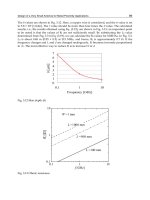
thus the read range of the tag will be increased. The proposed fractal curve has a greater
area under curve than the standard Koch curve in second iteration. Starting with an initiator
of length (

l), the second iteration area is (0.0766 l
2
cm
2
) for the proposed curve and (0.0688 l
2

cm
2
) for the standard Koch curve. According to equation (9) one can except to obtain a better
level of gain from proposed fractal loop higher than that from Koch fractal loop.
Fig. 22 shows the return loss (RL) of the designed loop antennas of 50Ω balanced feed port,
and Table 8 summarizes the simulated results of the designed loop antennas.

Read Range
(m)
Gain
(dBi)
eff.
(%)
Impedance
(Ω)
BW
(MHz)
Return Loss
(dB)
Antenna type
6.287 1.74 78.580.73-j7.3 31.4 -12.35 Standard Koch Loop
6.477 1.97 81.878.2-j8.9 36 -12.75 Proposed Loop
Table 8. Simulated results of the designed loop antennas.

Advanced Radio Frequency Identification Design and Applications

44

Fig. 22. Return loss of the two loop antennas.
From Table 8 it can be seen that the proposed fractal loop has better radiation characteristics
than the standard Koch fractal loop. As a result, higher read range is obtained. The
proposed fractal loop also is smaller in size than the standard Koch fractal loop. The
measured radiation pattern is in good agreement with the simulated one for the proposed
fractal loop antenna as shown in Fig. 23 .


(a) (b)
Fig. 23. The radiation pattern of the proposed fractal loop antenna: (a) measured,
(b) simulated (Salama& Quboa., 2008b).
Another new fractal curve is proposed as shown in Fig. 24 (Sabaawi et al, 2010) which
consists of five segments compared with standard Koch curve (60° indentation angle) which
consists of four segments, but has longer effective length (l
eff
=l . (3/2)
n
) compared with
(
l
eff
=l . (4/3)
n
) of standard Koch curve.
Design and Fabrication of Miniaturized Fractal Antennas for Passive UHF RFID Tags

45
a-Initiator
b-Generator

Fig. 24. First iteration of the proposed fractal curves: (a) initiator (n=0),(b) proposed fractal
curve generator (n=1).
The Affine transformation of the proposed fractal curve in the ω-plane can be described
according to equation (1), where θ is a rotating angle and
r is a scaling factor, while e and f
are translations involved in the transformation.

[
]
ferrrr ,,cos,sin,sin,cos
θ
θ
θ
θ
ω
−
=

(10)

⎥
⎦
⎤
⎢
⎣
⎡

= 0,0,
4
1
,0,0,
4
1
1
ω

⎥
⎦
⎤
⎢
⎣
⎡
−= 0,
4
1
,0,
4
1
,
4
1
,0
2
ω

⎥
⎦

⎤
⎢
⎣
⎡
=
4
1
,
4
1
,
2
1
,0,0,
2
1
3
ω

⎥
⎦
⎤
⎢
⎣
⎡
−=
4
1
,
4

3
,0,
4
1
,
4
1
,0
4
ω

⎥
⎦
⎤
⎢
⎣
⎡
= 0,
4
3
,
4
1
,0,0,
4
1
5
ω

54321

ω
ω
ω
ω
ω
ω
∪∪∪∪
=
t

Additional iterations can be performed by applying the Iterated Function System (IFS) to
each segment. Fig. 25 shows the first iterations P
0
, P
1
, and P
2
of the proposed fractal curve.

P
0
P
P
1
2

Fig. 25. First two iterations of the proposed fractal curves.
Advanced Radio Frequency Identification Design and Applications

46

A new fractal loop antenna is designed for passive UHF RFID tags at 900 MHz based on 2
nd

iteration of the above proposed curve with line width of (1mm). The fractal loop is split into
two halves (upper & lower halves) by making a horizontal cut at the centre of the loop as
shown in Fig. 26. The central-cut is used to control the impedance of the antenna and hence
increasing its matching.


Fig. 26. The proposed fractal loop antenna.
As shown in Fig. 25, the proposed fractal curve has a greater area under curve than that of
previous two loops in second iteration. Starting with an initiator of length (
l), the second
iterations area is (
0.1594 l
2
cm
2
) for the proposed curve in Fig. 26, and (0.0766 l
2
cm
2
) for the
fractal loop proposed in Fig. 21b (i.e more than twice the area).
The simulated results of the designed fractal loop include: input impedance (Z
a
), return loss
(RL) and radiation pattern will are shown in Figs. 27 & 28. These results will be useful in
understanding the benefits of the designed antenna like its small size as well as its radiation
properties.

Fig. 27. The simulated input impedance of the fractal loop antenna
74.42 mm
Design and Fabrication of Miniaturized Fractal Antennas for Passive UHF RFID Tags

47

Fig. 28. The simulated return loss of the fractal loop antenna
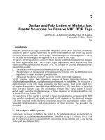
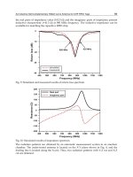
As shown from Figs. 27 & 28, the impedance of the antenna is (65.88+j3.4) Ω at 900 MHz
which is very close to the designing reference impedance of 50 Ω. It is also clear that the
return loss is (-26 dB) at 900 MHz with simulated -10 dB operating bandwidth of (59 MHz).
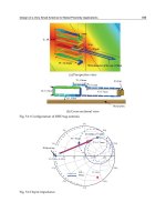
The simulated radiation pattern of the proposed fractal loop antenna is shown in Fig. 29.


(a) (b)
Fig. 29. The simulated Radiation Pattern. (a) 2D, (b) 3D.
One can see from the Fig. 29 that the radiation pattern at 900 MHz is almost omnidirectional
with deep nulls, and it is almost the same radiation pattern of an ordinary dipole with
simulated gain of (2.57 dBi). Table9 summarizes the simulated results of the proposed
fractal loop antenna compared with the fractal loop antenna published in (Salama and
Quboa, 2008b).
Advanced Radio Frequency Identification Design and Applications

48
Read Range
(m)
Gain
(dBi)
eff.

(%)
Impedance
(Ω)
BW
(MHz)
Return Loss
(dB)
Antenna
type
7.122 2.57 86.765.8+j3.4 59 -26 Proposed loop
Table 9. Simulated characteristics of the designed fractal loop antenna.
It is clear from Table 9 that the new proposed fractal loop has better radiation characteristics
from all those of the proposed fractal loop in (Salama and Quboa, 2008b) under the same
design conditions and parameters (i.e. the same substrate parameters), and as a result longer
read range is obtained which is the most important factor in designing RFID tags.
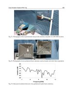
The proposed fractal loop antenna shown in Fig. 26 is fabricated using PCB technology as
shown in Fig. 27. A 50Ω coaxial cable type RG58/U and BNC connector is connected to the
fabricated antenna. In order to obtain balanced currents, Bazooka balun is used. The
performance of the fabricated antennas is verified by measurements. Radiation pattern is
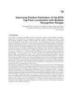
measured in anechoic chamber. The return loss of the fabricated loop antenna is measured
using MOTECH RF-2000 analyzer as shown in Fig. 28.


Fig. 27. The Fabricated Fractal Loop Antenna.


Fig. 28. Measured RL of the fabricated fractal loop antenna.