Advanced Radio Frequency Identification Design and Applications Part 4 pot

Design and Fabrication of Miniaturized Fractal Antennas for Passive UHF RFID Tags

49
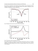
The measured return loss is (-17 dB) at a resonant frequency (889.62 MHz) compared with
the simulated one of (-26 dB) at 900 MHz, and the bandwidth is (19.2 MHz) compared with
the simulated bandwidth of (59 MHz). The disagreement between measured and simulated
results of the fractal loop antenna is attributed to the fact that we lack sufficient information
from the vendor of FR-4 material. This information would enable us to build accurate model
for the dielectric material in the EM simulator, instead of working with single frequency
point data.
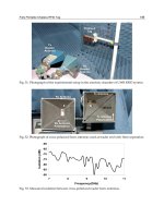
The radiation pattern for the fractal dipole antenna is measured in anechoic chamber as
shown in Fig. 29 which is in good agreement with the simulated results.


Fig. 29. Measured radiation pattern.
5. References
Andrenko A. S., (2005). Conformal Fractal Loop Antennas for RFID Tag Applications,
Proceedings of the IEEE International Conference on Applied Electromagnetics and
Communications, ICECom.
, Pages:1-6, Oct. 2008.
Balanis C. A., (1997), Antenna Theory Analysis and Design, Jhon Whily, New York, (2nd
Edition).
Baliarda C. P., Romeu J., & Cardama A., M. (2000), The Koch monopole: A small fractal
antenna.
IEEE Trans. on Antennas and Propagation, Vol.48, (2000) page numbers
(1773-1781).
Curty J. P., Declerdq M., Dehollain C. & Joehl N. , (2007).
Design and Optimization of Passive
UHF RFID Systems,
Springer, ISBN: 0-387-35274-0, New Jersey.
Sabaawi A. M. A., Abdulla A. I., Sultan Q. H., (2010), Design a New Fractal Loop Antenna

For UHF RFID Tags Based On a Proposed Fractal Curve, Proceedings of The 2
nd

IEEE International Conference on Computer Technology and Development (ICCTD
2010) November 2-4, 2010, Cairo, Egypt.
Sabaawi A. M. A., Quboa K. M., (2010). Sierpinski Gasket as Fractal Dipole Antennas for
Passive UHF RFID Tags. Proceedings of The Mosharaka International Conference
on Communications, Electronics, Propagation (MIC-CPE2010), 3-5 March 2010,
Amman, Jordan.
Advanced Radio Frequency Identification Design and Applications

50
Salama A. M. A., (2010). Antennas of RFID Tags, Radio Frequency Identification
Fundamentals and Applications Design Methods and Solutions, Cristina Turcu
(Ed.), ISBN: 978-953-7619-72-5, INTECH, Available from:

Salama A. M. A., Quboa K., (2008a). Fractal Dipoles As Meander Lines Antennas For Passive
UHF RFID Tags,
Proceedings of The IEEE Fifth International Multi-Conference on
Systems, Signals and Devices (IEEE SSD'08)
, Page: 128, Jordan, July 2008.
Salama A. M. A., Quboa K., (2008b). A New Fractal Loop Antenna for Passive UHF RFID
Tags Applications,
Proceedings of the 3
rd
IEEE International Conference on Information
& Communication Technologies: from Theory to Applications (ICTTA'08)
, Page: 477,
Syria, April 2008, Damascus.
Werner D. H. & Ganguly S. (2003). An Overview of Fractal Antenna Engineering Research.

IEEE Antennas and Propagation Magazine, Vol.45, No.1, (Feb. 2003), page numbers
(38-56).
Werner D. H., Haupt R. L., Werner P. L., (1999). Fractal Antenna Engineering: The Theory
and Design of Fractal Antenna Arrays.
IEEE Antennas and Propagation Magazine,
Vol.41, No.5, (1999) ,page numbers (37-58).
3
Design of RFID Coplanar
Antenna with Stubs over Dipoles
F. R. L e Silva and M. T. De Melo
Universidade Federal de Pernambuco
Brasil
1. Introduction
Radio Frequency Identification system, initially projected for objects identification in large
scale – a counterpart of the well-known barcode, has been expanding its horizons and has
been used for the automation of several services such as tracking goods, credit card
charging, supply chain controlling, and others. RFID systems consist on a Reader that
interrogates an identification Tag and this, in turn, sends an identification code back to the
Reader. Specifically, the passive RFID Tags take advantage of being free of batteries. It
converts part of the incoming RF signal from the reader into power supply. Because of its
versatility, lots of researchers have been investing on RFID, which, despite the 35 years old
of the first patent, is still considered new and somewhat obscure. This chapter covers topics
including the system surveying and the working basics of the RFID, especially the physical
air interface between the RFID tags (the mobile part) and the so-called Interrogators, which
are fixed part of the network. This chapter focuses on the project of 2.45 GHz planar
antennas, with a gain higher than the commercial ones, in such a way that, when these
brand new antennas are used in RFID tags, they increase the system efficiency. More
coverage area can be achieved with these higher gain antennas, as well as lower power
requirements of the Interrogators. Most of the necessary theory topics to project this antenna
are shown. As well as the theory, measured and simulated results are presented such as:

input impedance, frequency response, radiation pattern and gain, which could certainly be
the starting point for future works.
With respect to academic research over RFID, it is increasing year after year. The number of
publications in important periodicals is increasing in recent years. This happens due to its
great applicability in many areas like, health, commerce, safety, etc. In recent years, it is
becoming one of the most attractive areas in wireless applications. Figure 1 presents the
number of publications about RFID from 2003 to 2009 in the IEEE (Institute of Electric and
Electronics Engineers). As one can see, there is a considerable increase in recent years. This
Figure shows only the most relevant publications according to the algorithm of the IEEE
research in a sample space of 100 publications. In reality, the number of publications is in
the order of tens of hundreds.
In general the RFID system publications can achieve different focus. These can be about
development of antenna, chips identification, software control, etc. As usual, in all engineer
systems, there is something to improve. The system still is a bit expensive, as an Interrogator
may cost U$ 2,000.00. Another point is behind intersystem and intra-system interference, as
Advanced Radio Frequency Identification Design and Applications

52
it operates in the ISM bands (Industrial Scientific and Medical), free bands. Many others
systems, operating in that band, can interfere with RFID systems.


Fig. 1. RFID Publication in the IEEE. It is included publications over performance
evaluation, development of news tools, new hardwares, etc.

Publicações sobre antenas para RFID no IEEE*
0
5
10
15

20
25
30
35
40
45
2002 2003 2004 2005 2006 2007 2008 2009
Ano
N° de publicações

Fig. 2. Number of publications specifically for RFID antennas in the IEEE, in a sample space
of 100 publications.
Publicaçõe s sobre RFID no IEEE**
0
5
10
15
20
25
30
35
40
45
2003 2004 2005 2006 2007 2008 2009
Ano
N° de publicações
year
N
o
of

p
ublication
RFID Publications in the IEEE
year
N
o
of
p
ublications
RFID antennas Publication in the IEEE
Design of RFID Coplanar Antenna with Stubs over Dipoles

53
For a matter of power saving, design of high gain antenna can be necessary in the case of
longer distance reading. On the other hand, some specific radiation patterns are suitable for
grouped tags, avoiding the interfering effects. Besides, some Interrogators antenna arrays,
can optimize the system power consume and/or optimize the number and position of the
Interrogators, decreasing both the cost of implementation and the maintenance. It is clear
that there is no any unique solution for whole problems, and perhaps, a particular solution
for a particular problem. Figure 2 also shows an increase in the number of publications
specifically for RFID antennas from 2002 to 2009 in the IEEE. These are only publications in
the IEEE, there are other important periodicals, conferences, meeting, symposiums, etc.
about RFID all over the world. Certainly, in this research area there is much work to do
about optimization and cost reduction.
As the antenna design is one of the most important parts of RFID system development, it
becomes necessary to see some basic concepts, analysis, and characterization of antennas
used in RFID applications.
2. Important concepts
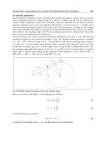
As predicted by Friis (Balanis, 1982) in (1), the reading range r is a function of the following
parameters: wavelength in the free space λ, EIRP power P

t
·G
t
, tag antenna gain G
r
and the
minimum required power for activating the RFIC chip P
r
(Karthaus & Fischer, 2003). RFIC
operating with 16.7μW minimum power level (Karthaus & Fischer, 2003) and indoor Reader
EIRP of 27dBm, gain improvements on the tag antenna could increase the reading range of
the system. Figure 3 shows the system reading range as a function of the antenna gain.
According to (Karthaus & Fischer, 2003), (Finkenzeller), passive RFIC tags have generally
negative input reactance and may have low input resistance. The impedance of the RFIC
and the antenna must be matched each other (Finkenzeller).

4
ttr
r
PGG
r
P
λ
π
⋅
⋅
=
⋅
(1)

Fig. 3. Reading range versus tag antenna gain.
Advanced Radio Frequency Identification Design and Applications

54
3. Tag antenna design
Let us see the design step by step. It consists of two λ/2 folded dipole array fed by λ/4
Transmission Line (TL) sections. Each folded dipole works like a load for a λ/4 transmission
line (TL). As described in (de Melo et al., 1999), two loaded λ/4 TL are connected at the
position A-A´. This yields to array of two planar dipoles. The transmission lines TL, as
shown in Figure 4, of length λ/4 works like an impedance transformer for the required
input impedance at the feeding points A-A’. From Figure 5, one can see the load in the
shape of a planar folded dipole.


Fig. 4. Loaded CPS transmission lines.


Fig. 5. Load in the shape of a dipole.
The transmission lines are connected together at the terminals A-A’, as shown in Figure 4.
Arrays of radiating elements produce higher gain than isolated elements (Balanis, 1982).
This fact allows this antenna to be useful when farther reading ranges are required. Because
its symmetry related to the central plane, only half the antenna is analyzed and the results
are further corrected in order to represent the whole antenna. With the dimensions
described in Table 1 (Condition 1), the input impedance of one dipole can be calculated
using quasi-static equations of conformal mapping (Lampe, 1985), (Nguyen, 2001), (de Melo
et al., 1999) and such impedance is referred to as Z
dipole
. It is the load impedance for the
transmission line.

In practice it is not simple to obtain the dipole impedance, taking into account the real
values of the geometrical parameters. The known usual expressions are suitable for ideal
conditions and do not take into account some parameters, like width D, shown in the
Figure 6. Another example is the gap G created in one of the strips for the signal feeding.
Besides, the lower strip becomes smaller, comparing with the upper one. However, the
expressions, published by (Lampe, 1985) still may be used to have an idea of the dipole
behavior with variation of line width, space between strips, etc. To obtain the dipole
impedance
di
p
ole d d
ZR
j
X
=
+ some simulations were carried out using the full wave
simulator CST, varying the dipole geometric parameters.
Design of RFID Coplanar Antenna with Stubs over Dipoles

55

Fig. 6. Dimensions and parameters of the coplanar strip folded dipole.
Figures 7(a) and 7(b) present the real and imaginary part of the input impedance as a
function of W1, respectively. Figures 8(a) and 8(b) present the real and imaginary part of the
input impedance as a function of W2, respectively. Following the same idea, Figures 9 and
10 present the input impedance variations with S and D dimensions, respectively.


Fig. 7. Input impedance as a function of W1. (a) is the real part and (b) is the imaginary part.

Fig. 8. Input impedance as a function of W2. (a) is the real part and (b) is the imaginary part.
W1(mm)

(
a
)
W1(mm)

(
b
)



W2(mm)

(
a
)
W2(mm)

(
b
)

Advanced Radio Frequency Identification Design and Applications

56

Fig. 9. Input impedance as a function of
s. (a) is the real part and (b) is the imaginary part.


Fig. 10. Input impedance as a function of
D. (a) is the real part and (b) is the imaginary part.
The half-antenna input impedance at the plane A-A’ (Figure 4) is given by the usual
equation for transmission lines (Chang, 1992):

(
)
()
dipole 0
in 0
0dipole
ZZtanhγL
ZZ
ZZ tanhγL
+
=
+
(2)
where
γ is the propagation constant of the wave, L is the transmission line section length
and Z
0
is the characteristic impedance of the transmission line. The value of Z
0
is also
calculated by quasi-static conformal mapping equations.

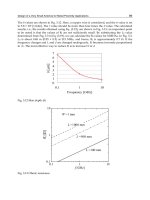
Figure 11 shows a coplanar folded dipole design. This structure is more suitable for
matching with only the real part of the input impedance. Figures 12(a) and 12(b) present the
real and imaginary part of the input impedance as a function of the length of the stub
l,
respectively. The imaginary part goes from negative to positive values as the length
l
increases from 0(mm) to 20(mm). For a fixed value of
l, Figures 12(a) and 12(b) can be used
for impedance match between the antenna and the chip or between the antenna and the
network analyzer. Note that the input impedance also can change with the spacing g, the
width k and the distance H.


s(mm)

(
a
)
s(mm)

(
b
)

D(mm)

(
a
)
D(mm)

(
b
)
Design of RFID Coplanar Antenna with Stubs over Dipoles

57
feed terminal

Fig. 11. Dimensions and parameters of the coplanar strip folded dipole.


Fig. 12. Input impedance as a function of
l. (a) is the real part and (b) is the imaginary part.


Fig. 13. Antenna layout. The stubs are placed over the dipoles.
l(mm)

(
a
)
l(mm)

(
b
)

Advanced Radio Frequency Identification Design and Applications

58
Dimensions
Condition 1
Condition 2
h
53 mm
53 mm
w
4 mm
4 mm
a
3 mm
3 mm
d1
8.5 mm
8.5 mm
d2
8.5 mm
8.5 mm
L
26.5 mm
26.5 mm
T
38.5 mm
38.5 mm
A
0 mm
14 mm
Table 1. Dimensions of the antenna
Note that all dimensions have the same value for condition 1 and 2, except for

A . The
A = 0 mm means no stubs. For all dimensions described in Table 1 - condition 1, the input
impedance of half the antenna is Z 100 j100Ω
in
=
+ . Because its symmetry, the impedance of
whole antenna at the plane A-A´ is to be
Z
in
Z
ant
2
=
. In other words, Z 50 j50Ω
ant
=+ .
The imaginary part of
Z
ant
can be significantly decreased by placing planar stubs over the
dipoles. On the other hand, the real part of
Z
ant
is slightly altered. Those facts are important
when purely real impedance is needed. That is the case when stubs of length
A = 14mm are
added to the dipoles (Table 1 - Condition 2). At that length, the above described impedance
becomes
Z49Ω
ant

= and the imaginary part is no longer seen.
4. Fabrication measurement and simulation
The antenna described in the previous section was simulated with a full wave EM software.
The fabricated antenna with stubs over the dipoles is shown in Figure 14. It was
implemented on a RT6002 substrate of thickness 1.5mm, relative dielectric permittivity
ε
r
= 2.94 and loss tangent δ = 0.0012. Simulations were taken in the 1.5 – 3 GHz range.
Calculations of input impedance were taken at 2.45GHz, which is the central frequency of
the free 2.4GHz part of the spectrum. Figure 15, 16 and 17 show the comparison between
simulated and measured results and good agreement can be noticed. Figure 18 and 19 show
the radiation pattern and the gain of this proposed antenna at 2.45GHz. The antenna lies in
the plane
θ = 90° and has its printed strips at the right-hand side. The maximum gain is
increased over the direction perpendicular to the antenna plane. Still from Fig. 7, one sees
that the highest simulated gain reaches 5.97dB over an isotropic radiator. The measured gain
reaches 5.6dB, which is very close to the simulated one. These values are at least twice
higher than the gain of an ordinary dipole (Finkenzeller). Simulated results show how the
stub length can modify the Z
dipole
and the antenna input impedance Z
ant
, as a consequence.
Thus, it is possible to choose some suitable stub length for the desired antenna input
impedance. For example, for
A = 14 mm, one finds the simulated antenna input impedance
of
Z50j7Ω
ant
=+ . It is very close to that one of 49

Ω
, expected in the section before. On the
other hand, the measured value of the new antenna is
ant
Z48j7Ω=+
.
Design of RFID Coplanar Antenna with Stubs over Dipoles

59

Fig. 14. The printed antenna.

f
requenc
y
(GHz)
Impedance - real part (Ohms)
measured
simulated

Fig. 15. Simulated and measured real part of the impedance.

frequency (GHz)
Impedance - imaginary part (Ohms)
measure
d
simulated

Fig. 16. Simulated and measured imaginary part of the impedance.
Advanced Radio Frequency Identification Design and Applications

60
In the Figure 16 one notices a slight difference between the simulated and measured
responses, at the central frequency. This may be explained due to a possible coupling
between the two radiator elements.


Fig. 17. Comparison of the simulated and measured return loss for the antenna shown in
Figure 14.


Fig. 18. Simulation results of radiation pattern, directivity, gain and radiation efficiency for
the antenna in Figure 14.
Design of RFID Coplanar Antenna with Stubs over Dipoles

61
For the gain calculation of the antenna in Figure 14, one takes the value from Figure 18.
Directivity D = 6,011 dB and radiation efficiency
η = 0,003689. Thus, one finds
G = 6,011-0,003689
≅ 5,97dB.


Fig. 19. Simulated and measured antenna gain over an isotropic antenna: 5.97dB and 5.6dB,
respectively.
5. Conclusion
Good agreement between simulated and measured responses is seen. The reading range of
RFID Tags can be increased by 41 % when this antenna is used. Stubs over the dipoles are a
very useful tool when impedance adjustments are needed. This antenna has good
performance comparing with the commercial versions available and seems to be promising

as far as RFID applications are concerned. For the future some improvements can be carried
out over the design. Decrease the whole size, modeling equation approach for the gaps,
discrete elements equivalent circuit elaboration and insertion of this antenna into an active
RFID system.
6. References
C. A., Balanis. (1982). “Fundamental Parameters of Antennas”, Antenna Theory – Analysis
and Design, 2
nd
ed., New York, NY, USA: John Wiley & Sons, Chapter 2, p. 88.
U. Karthaus and M. Fischer. (2003). “Fully Integrated Passive UHF RFID Transponder IC
With 16.7
μW Minimum RF Input Power”, IEEE Journal of Solid State Circuits, vol. 38,
no. 10, pp. 1602-1608, Oct.
Advanced Radio Frequency Identification Design and Applications

62
K. Finkenzeller, RFID Handbook: Fundamentals and Applications in Contactless Smart
Cards and Identification, 2
nd
edition, New York, NY, USA: John Wiley & Sons,
pp.121, 133-136.
R.W. Lampe, (1985). “Design Formulas for an Asymmetric Coplanar Strip Folded Dipole”,
IEEE Trans. Antennas and Propagat., vol. AP-33, no.9, pp. 1028-1031, Sep.
C. Nguyen, (2001). “Conformal Mapping”, Analysis Methods for RF, Microwave and
Millimeter-Wave Planar Transmission Line Structures, 1
st
ed., New York, NY, USA:
John Wiley & Sons, Chapter 5, pp. 109-111.
M. T. de Melo, M. J. Lancaster, J. S. Hong, E. J. P. Santos and A. J. Belfort. (1999).“Coplanar
Interdigital Delay Line Theory and Measurement”.

Proceedings of the 29TH
EUROPEAN MICROWAVE CONFERENCE, Munich, Miller Freeman
, v. 3, p. 227-230.
D. K. Cheng. (1992). “Theory and Applications of Transmission Lines”, Field and Wave
Electromagnetics, 2
nd
ed., New York, NY, USA: Addison-Wesley, Chapter 9, p. 451.
4
An Inductive Self-complementary
Hilbert-curve Antenna for UHF RFID Tags
Ji-Chyun Liu
1
, Bing-Hao Zeng
1
and Dau-Chyrh Chang
2

1
Ching Yun University Chung-Li City, Taoyuan County, Taiwan
2
Oriental Institute of Technology Pan-Chiao City, Taipei County, Taiwan
R.O.C
1. Introduction
Recently there has been a rapidly growing interest in RFID systems and its applications.
Operating frequencies including 125 KHz–134 KHz and 140 KHz–148.5 KHz LF band, 13.56
MHz HF band and 868 MHz–960 MHz UHF band were applied to various supply chains.
433 MHz band was decided for active reader and 2.45 GHz band was applied for WiFi
reader. Besides the reader antennas, the requirements of tag antennas are necessary for
applications. In which, due to the benefit of long read range and low cost, the UHF tag will
be used as the system of distribution and logistics around the world [1–13], [29–41].

Meander line antennas were commonly for UHF tags, due to the characteristics of high gain,
omni-directionality, planarity and relatively small surface size [5]. However, the length-to-
width ratio limited as 5:1 was proposed [2]. Recently, the half-Sierpinski fractal antenna was
introduced with a small length-to-width ratio (<2:1) [11]. Meanwhile, the inductive
impedance of tag antenna was necessary for matching the capacitive terminations of chip
IC, thus the tuning apparatus was proposed [4], [8]–[10]. H-shaped meandered-slot
antennas with the performance of broadband and conjugate impedance matching were
developed for on-body applications [14], [15]. On the other hand, the self-complementary
dipoles were introduced for the performance of wideband, high impedance and balun
[16]–[23].
The Hilbert-curve, proposed by Hilbert and introduced by Peano [24], was known as the
space-filling curves. The structure of this shape can be made of a long metallic wire
compacted within a patch. As the iteration order of the curve increases, the Hilbert-curve
can be space-filling the patch. It has been used in fractal antenna with size reduction [25–28],
[44–52].
The main aim of this paper is to merge the meander line and meandered-slot structure of the
RFID tag antenna in order to obtain a good performance of compact, broadband and
conjugate impedance matching. Meantime, demonstrating the performance with a self-
complementary Hilbert-curve tag antenna is proposed. The self-complementary Hilbert-
curve tag antenna is constructed with substrate, Hilbert-curve, Hilbert-curve slot and tuning
pad. For circular polarization analysis, the current distribution and electric field are
exhibited. The inductive and broadband characteristics of frequency responses and
directivity feature of radiation patterns and polarization are studied and presented.
Advanced Radio Frequency Identification Design and Applications

64
2. Antenna configuration and basis
2.1 UFH RFID meander-line antenna
The typical dipole antenna consists of two parts, in Fig.1, one is the dipole resonators with
half-wavelength for resonance and the other is the balun for the impedance transfer of

balance to unbalance terminations. The standing voltage and current distribute among the
dipole with maxima current and minimum voltage feeding in the center (0°) for linear
polarization. For size reduction, in Fig.2, the meander-line configuration was applied in tag
antenna. By tuning load-line structure, more wideband and inductive performance can be
achieved.


Fig. 1. Dipole antenna


Fig. 2. Meander line antennas
2.2 Hilbert-curve and space filling
Hilbert-curve is a space filling curve with being self-similar and simple geometry. The
configurations of Hilbert-curve for first four fractal iterations are shown in Figure 3. The
original space has filling nature of these curves. This expresses that for a given area of a
space, the total length of the line segments increase progressively as the iteration order
increases. It can be interpreted as the cause for their relatively lower resonant frequency. It is
evident that the fractal iteration order increases, the total length of the line segments
An Inductive Self-complementary Hilbert-curve Antenna for UHF RFID Tags

65
increases, even as the area it encompasses remain the same. Thus within a small area, a
lower resonant frequency antenna with very large line length can be accommodated. In
applications, the structure of this shape can be made of a long metallic wire compacted
within a microstrip patch.
The topological dimension of the line segments is one, as it consists only of a line. The
dimension of this original space is an integer value equated two. When we consider the
length and number of line segments with 2
nd
, 3

rd
and 4
th
iterations, this dimension are 1.465,
1.694 and 1.834. These values point to the fact the geometry has fractional dimension. As the
dimension approaches 2, the curve almost fills a space. In other words, for large iteration
orders, the total length of the line segments tends to be extremely large. This could be a
significant advantage in lower frequency antenna design since the overall effective length of
the antenna is large. Thus the resonant frequency can be reduced considerably for a given
area, by increasing the fractal iteration order. It may result in a larger reduction factor for
the antenna size.


(a) (b) (c) (d) (e)
Fig. 3. First four fractal iterations for the Hilbert-curve configurations, (a) original space (b)
1
st
iterations (c) 2
nd
iterations (d) 3
rd
iterations (e) 4
th
iterations
2.3 Self- complementary antennas
Self-complementary antenna composed with electric and magnetic pair antennas is a
potential antenna solution for multi-band and wide-band antenna system because of its
excellent isolation performance at close proximity between antennas. The pair antennas can
be configured with log-period, spiral and circular disk configuration depends on application
shown in Fig. 4.

Antenna pair with self-complementary structure has a constant input impedance, independent
of the source frequency and the antenna geometry. To achieve wideband CP performance,
self-complementary structures were commonly used owing to their features of simple
feeding and good axial ratio [17, 18, 23].
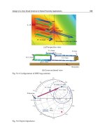
2.4 Self-complementary Hilbert-curve tag antenna
Complementary Hilbert-curve tag antenna is constructed with substrate, Hilbert-curve,
Hilbert-curve slot and tuning pad (L
t
) in Fig. 5. The Hilbert-curve is consisted of three
series Hilbert-curve with the 3rd iteration. The dimensions are L
1
= 23.5 mm, L
2
= 24 mm,
L
t
= 5mm, W
1
= 7.5 mm, W
2
= 8.5 mm, W
3
=0.75 mm, W
4
= 0.5 mm, and g =0.35 mm. The
thickness (h) of RT/duroid-6010 substrate is 6.35 mm (1.27mm×5) and the relative
permittivity ε
r
is 10.2 shown in Fig. 6. The length-to-width ratio is 6.2:1 and the shortening
ratio SR=0.69. The reduction is notable when the SR is more than 0.40 [2].

Advanced Radio Frequency Identification Design and Applications

66

(a)

(b)

(c)
Fig. 4. Self-complementary antenna configurations, (a) log-period (b) spiral (c) circular disk
A typical circular polarization dipole cross-pair usually consist of two individuals with
horizontal and vertical locations, and a two-phase signal with 90° difference. Fig. 7
illustrates the simulated current distributions and Fig. 6 depicts the simulated electric fields
among the planar structures, which provide a clearly physical insight on understanding the
circular polarization of the proposed antenna. Fig. 5 shows that the Hilbert-curve is excited
An Inductive Self-complementary Hilbert-curve Antenna for UHF RFID Tags

67
with concentrating current distributions at the 900 MHz resonance while the maximum
amplitude located at –11.3° with deviation from central feed-line (0°). The Hilbert-curve slot
is expressed with lower current distributions. Fig. 8 presents both Hilbert-curve line and
Hilbert-curve slot are excited with intensive electric fields at the 900 MHz resonance while
the minimum amplitude presented at –22.5°.


Fig. 5. Complementary Hilbert-curve antenna


Fig. 6. Dimensions of complementary Hilbert-curve tag antenna
Since the phase difference with 33.8° among maximum current amplitude and minimum

electric field existed, in company with the different locations of the left Hilbert-curve line
and the right Hilbert-curve slot, the elliptic polarization will be obtained. Thus, the circular
polarization can be observed along a certain direction.
Advanced Radio Frequency Identification Design and Applications

68

Fig. 7. Current distributions


Fig. 8. Electric fields
2.5 Applications
The maximum activation distance of the tag for the given frequency is given [14]–[15] by

max
4
R
chip
EIRP
c
dG
fP
τ
π
= (1)
Where EIRP
R
is the effective transmitted power of reader, P
chip
is the sensitivity of tag

microchip, G is the maximum tag antenna gain, and the power transmission factor

2
4
1
chip A
chip A
RR
XX
τ
=
≤
+
(2)
with tag antenna impedance (
AA A
Z
RjX
=
+ ) and microchip impedance ( chip chip chip
Z
RjX
=
+ ).
3. Simulations and experiments
By using the commercial software of HFSS tool [42], the simulation results included return
loss spectrums, impedance spectrum, circular polarization and two-cut radiation patterns
are presented and analyzed. For comparison, the return loss spectrums of the proposed
antenna with UHF-bands of 900 MHz are measured and simulated shown in Fig. 9.
The simulated and measured results of frequency responses are in agreement. In

measurement, while the return loss is smaller than -10dB, the frequency responses cover
both Europe 865.6–867.6 MHz band and USA 902–928 MHz band, ranging from 820 to 935
MHz (bandwidth = 115 MHz). For applications, the frequency responses are fully applied in
the operation bands of the RFID UHF-band. For impedance spectrum analysis in Fig. 10, it
shows the real parts of impedance become maximum value (178.7 Ω) at 970 MHz frequency,