Artificial Neural Networks Industrial and Control Engineering Applications Part 4 pot

Artificial Neural Networks - Industrial and Control Engineering Applications

94
composition elements were known based on the type of mineral. Powder-based samples are
used to train, validate and test the composition retrieval algorithm, while the natural rocks
and minerals are used only to test the mineral identification capability.


Fig. 1. Experimental configuration of a LIBS system.

270 280 290 300 310 320 330 340 350
Wavelength (nm)
AndesiteJA1
Rock71306
Concentration (fraction)
Std name SiO
2
Al
2
O
3
MgO CaO Na
2
OK
2
OTiO
2
Fe
2
O
3

MnO
Rock71306 0.0062 0.001 0.218 0.3002 0.0003 0.00038 0.00015 0.0021 0.00108
AndesiteJA1 0.6397 0.1522 0.0157 0.057 0.0384 0.0077 0.0085 0.0707 0.00157

Fig. 2. Examples of LIBS spectra for materials with different composition.
Let us consider few examples of raw LIBS spectra. Spectral signatures of a carbonate rock
(Rock 71306) and an andesite (JA1) are shown in Fig. 2. Due to large difference in
compositions of these two materials, their discrimination can be easily arranged. Here, a
monitoring of intensities of several key atomic lines (Si, Al, Ca, Ti and Fe in this case) can be
employed. Therefore, identification or classification of types of minerals with a strong
difference in composition can be easily achieved using simple logic algorithms. In this case,
we rather care about the presence of specific spectral lines than the exact measurement of
their intensity and correspondence to elemental concentration.
Nd: YAG laser
Sample
Pulse delay
generator
Lens
Mirror
Beam Splitter
Mirror
Polarizer
λ
/2 Plate

Spectrometer
Joule-meter
Computer
Artificial Neural Networks for Material Identification, Mineralogy and
Analytical Geochemistry Based on Laser-Induced Breakdown Spectroscopy

95
The situation however, can be much more complex when one deals with identification of
materials with high degree of similarity, or with retrieval of compositional data
(quantitative analysis). Such an example is presented in Fig. 3. Here the strategy for these
two applications may diverge. Such, that for material identification the spectral lines
showing the largest deviations between materials (Mg in this example) should be used.
However, for quantitative analysis it is rather useful to select the spectral lines that exhibit
near-linear correspondence of the intensity and the element concentration (Ti 330 nm – 340
nm lines in this example). This is why the material identification and quantitative analysis
that will be discussed in the following sections rely on different spectral line selection.

270 280 290 300 310 320 330 340 350
Wavelen
g
th
(
nm
)
Andes iteJA1
Andes iteJA2
Concentration (fraction)
Std name SiO
2
Al
2
O
3
MgO CaO Na
2

OK
2
OTiO
2
Fe
2
O
3
MnO
AndesiteJA1 0.6397 0.1522 0.0157 0.057 0.0384 0.0077 0.0085 0.0707 0.00157
AndesiteJA2 0.5642 0.1541 0.076 0.0629 0.0311 0.0181 0.0066 0.0621 0.00108

Fig. 3. Examples of LIBS spectra for materials with similar composition.
Once LIBS spectra are acquired from the sample of interest, several pre-processing steps are
performed. Pre-processing techniques are very important for proper conditioning of the
data before feeding them to the network and account for about 50 % of success of the data
processing algorithm. The following major steps in data conditioning are employed before
the spectral data are inputted to the ANN.
a. Averaging of LIBS spectra. Usually, averaging of up to a hundred of spectral samples
(laser shots) may be used to increase signal to noise ratio. The averaging factor depends
on experimental conditions and the desired sensitivity.
b. Background subtraction. The background is defined as a smooth part of the spectrum
caused by several factors, such as, dark current, continuum plasma emission, stray
light, etc. It can be cancelled out by use of polynomial fit.
c. Selection of spectral lines for the ANN processing. Each application requires its own set
of selected spectral lines for the processing. This will be discussed in greater details in
the following sections.
d. Calculation of normalised spectral line intensities. In order to account for variations in
laser pulse energy, sample surface and other experimental conditions the internal
normalization is employed. In our studies, we normalize the spectra on the intensity of O

777 nm line. This is the most convenient element for normalization since all our samples
contain oxygen and there is always a contribution of atmospheric oxygen in the spectra in
normal ambient conditions. The line intensities are calculated by integrating the
corresponding spectral outputs within the full width half-maximum (FWHM) linewidth.
Artificial Neural Networks - Industrial and Control Engineering Applications

96
After this pre-processing, the amount of data is greatly reduced to the number of selected
normalized spectral line intensities, which are submitted to the ANN.
3. ANN processing of LIBS data
The ANN usually used by researchers to process LIBS data and reported in our earlier
works is a conventional three-layer structure, input, hidden, and output, built up by
neurons as shown in (Fig. 4). Each neuron is governed by the log-sigmoid function. The first
input layer receives LIBS intensities at certain spectral lines, where one neuron normally
corresponds to one line.
A typical broadband spectrometer has more than a thousand channels. Inputting to the
network the whole spectrum increases the network complexity and computation time. Our
attempts to use the full spectrum as an input to ANN were not successful. As a result, we
selected certain elemental lines as reference lines to be an input to ANN. General criteria for
the line selection are the following: good signal to noise ratio (SNR); minimal overlapping
with other lines; minimal self-absorption; and no saturation of the spectrometer channel.


Fig. 4. Basic structure of an artificial neural network.
These criteria eliminate many lines which are commonly used by other spectroscopic
techniques. For example, the Na 589 nm doublet saturates the spectrometer easily, thus is
not selected. The C 247.9 nm can be confused with Fe 248.3 nm, therefore is avoided. At the
same time, the relatively weak Mg 881 nm line is preferred to 285 nm line since it is located
in a region with less interference from other lines. In addition to these general rules, some
specific requirements for line selection imposed by particular applications are discussed in

the following sections.
The number of neurons in the hidden layer is adjusted for faster processing and more
accurate prediction. Each neuron at the output layer is associated either to a learnt material
(identification analysis) or an element which concentration is measured (quantitative
analysis). The output neurons return a value between 0 and 1 which represents either the
confidence level (CL) in identification or a fraction of elemental composition in quantitative
processing.
The weights and biases are optimized through the feed-forward back-propagation
algorithm during the learning or training phase. To perform ANN learning we use a

Neuron
Layer 2Layer 1 Layer 3
p
1

I(
λ
1
)
Output n
p
2

p
n

I(
λ
2
)

I(
λ
n
)
Inputs x
i

Bias b
Weights w
i

⎟
⎠
⎞
⎜
⎝
⎛
−=
∑
i
ii
bxwfn
u
e
uf
−
+
=
1
1

)(
Artificial Neural Networks for Material Identification, Mineralogy and
Analytical Geochemistry Based on Laser-Induced Breakdown Spectroscopy

97
training data set. Then to verify the accuracy of the ANN processing we use validation data
set. Training and validation data sets are acquired from the same samples but at different
locations (Fig. 5). In this particular example ten spectra collected at each location and
averaged to produce one input spectrum per location. Five cleaning laser shots are fired at
each location before the data acquisition.

Learning set
Validation set

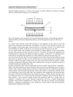
Fig. 5. Acquiring learning and validation spectra from a pressed tablet sample. The ten spots
on the left are laser breakdown craters corresponding to the data sets. An emission
collection lens is shown on the right in the picture.
3.1 Material identification
Material identification has been demonstrated recently with a conventional three-layer feed-
forward ANN (Koujelev et al., 2010). High success rate of the identification algorithm has
been demonstrated with using standard samples made of powders (Fig. 6). However, a need
for improvements has been identified to ensure the identification is stable with given large
variations of natural rocks in terms of surface condition, inhomogeneity and composition
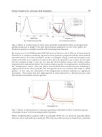
variations (Fig. 7). Indeed, the drop in identification success rate between validation set and
the test set composed of natural minerals and rocks is from 87 % to 57 % (Fig. 6). Note, at the
output layer, the predicted output of each neuron may be of any value between 0 (complete
mismatch) and 1 (perfect match). The material is counted as identified when the ANN
output shows CL above threshold of 70 % (green dashed line). If all outputs are below this
threshold, the test result is regarded as unidentified. Additional, soft threshold is introduced
at 45 % (orange dashed line) such that if the maximum CL falls between 45 % and 70 %, the

sample is regarded as a similar class.
An improved design of ANN structure incorporating a sequential learning approach has
been proposed and demonstrated (Lui & Koujelev, 2010). Here we review those
improvements and provide a comparative analysis of the conventional and the constructive
leaning network.
Achieving high efficiency in material identification, using LIBS requires a special attention
to the selection of spectral lines used as input to the network. In addition to the above
described considerations, we added an extra rational for the line selection. Lines with large
variability in intensity between different materials, having pronounced matrix effects were
preferred. In such a way we selected 139 lines corresponding to 139 input nodes of the
ANN. The optimized number of neurons in the hidden layer was 140, and the number of
output layer nodes was 41 corresponding to the number of materials used in the training
phase.
Artificial Neural Networks - Industrial and Control Engineering Applications

98
0 0.1 0.2 0.3 0.4 0.5 0.6 0.7 0.8 0.9 1
andesite AGV2
andesite JA1
andesite JA2
andesite JA3
anorthosite 2120
anorthosite 1042
basalt BCR2
basalt BHVO2
basalt JB2
black soil
borax frit
coulsonite
Cu-Mo

flint clay
granite
graphite
grey soil
ilmenite
iron ore
kaolin
K-feldspar
Mn ore
obsidian rock
olivine
orthoclase gabbro
pyroxenite
red clay
red soil
rhyolite
dolomite
andesite GBW07104
iron rock
alumosilicate sediment
shale
sillimanite
sulphide ore
syenite JSy1
syenite SARM2
talc
ultrabasic rock
wollastonite
andesite
basalt

gabbro
dolomite
graphite
hematite
kaolinite
obsidian
olivine
shale
sulfide mixture
talc
fluorite
molybdenite
CL (fraction)
test set (natural rocks & minerals)validation set (powders)

Fig. 6. Identification results for ANN with conventional training: powder tablets validation
and natural rock & mineral test. Green colour corresponds to confidence levels for correct
identification and red colour corresponds to mis-identification ANN outputs.
Artificial Neural Networks for Material Identification, Mineralogy and
Analytical Geochemistry Based on Laser-Induced Breakdown Spectroscopy

99
Andesite Basalt Gabbro Dolomite Graphite Hematite Kaolinite


NA
Obsidian Olivine Shale Sulfide
mixture
Talc Fluorite Molybde-
nite

NA NA
Fig. 7. Natural rock & mineral samples and their powder tablets counterparts.

1
st
ANN trainin
g
2
nd
ANN trainin
g
3
rd
ANN trainin
g
4
th
ANN trainin
g
5
th
ANN trainin
g
Randoml
y
initialized wei
g
hts & biases

Wei
g
hts & biases from the 1
st
trainin
g
1
st
trainin
g

subset
2
nd
training
subset
3
rd
training
subset
4
th
training
subset
5
th
training
subset
Wei
g

hts & biases from the 2
nd
trainin
g
Wei
g
hts & biases from the 3
rd
trainin
g
Wei
g
hts & biases from the 4
th
trainin
g
Trained ANN

Fig. 8. Sequential training diagram.
When dealing with a conventional training the identification success rate drops rapidly if
natural rock samples are subject to measurement on the ANN trained with powder made
samples. This is, as we believe, due to overfitting of ANN. To avoid overfitting, the number
of training cases must be sufficiently large, usually a few times more than the number of
variables (i.e., weights and biases) in the network (Moody, 1992). If the network is trained
1cm
Artificial Neural Networks - Industrial and Control Engineering Applications

100
only by the average spectrum of each sample corresponding to 41 training cases, then the
ANN is most likely to be overfitted. To improve the generalization of the network, the

sequential training was adopted as an ANN learning technique (Kadirkamanathan et al.,
1993; Rajasekaran et al., 2002 and 2006).
The early stopping also helps the performance by monitoring the error of the validation data
after each back-propagation cycle during the training process. The training ends when the
validation error starts to increase (Prechelt, 1998). In our LIBS data sets there are five
averaged spectra per sample, each used in its own step of the training sequence. At each
step, the ANN is trained by a subset of spectra with the early stopping criterion and the
optimized weights and biases are transferred as the initial values to the second training with
another subset. This procedure repeats until all subsets are used.
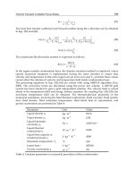
The algorithm implementation is illustrated in (Fig. 9). While the mean square error (MSE)
decreases going through 5 consecutive steps (upper graph), the validation success rate
grows up (bottom graph).


Fig. 9. Identification algorithm programmed in the LabView environment: the training
phase.
Using a standard laptop computer the learning phase is usually completed in less than 20
minutes. Once the learning is complete, the identification can be performed in quasi real
time. The LIBS-ANN algorithm and control interface is shown in (Fig. 10).
Identification can be performed on each single laser shot spectrum, on the averaged
spectrum, or continuously. The acquired spectrum displayed is of the Ilmenite mineral
sample in the given example. When the material is identified, the composition
corresponding to this material is displayed. Note, that the identification algorithm does not
calculate the composition based on the spectrum, but takes the tabular data from the
training library. The direct measurement of material’s composition is possible with
quantitative ANN analysis.
In the event if the sample shows low CL for all ANN outputs it is treated as unknown. In
such a case, more spectra may be acquired to clarify the material identity. If it is confirmed
by several measurements that the sample is unknown to the network, it can be added to the
Artificial Neural Networks for Material Identification, Mineralogy and

Analytical Geochemistry Based on Laser-Induced Breakdown Spectroscopy

101
training library and the ANN can be re-trained with the updated dataset. Thus, for a remote
LIBS operation, this mode "learn as you go" adds frequently encountered spectra on the site
as the reference spectra. This mode offers a solution for precise identification without
dealing with too large database of reference materials spectra beforehand. The exact identity
or a terrestrial analogue (in case of a planetary exploration scenario) can be defined based on
more detailed quantitative analysis, possibly, in conjunction with data from other sensors.


Fig. 10. Identification algorithm programmed in the LabView environment: how it works for
a test sample that has been identified. Upper-left section defines the hardware control
parameters. Bottom-left section defines the spectral analysis parameters (spectral lines).
Top-right part displays the acquired spectrum. Bottom-right section displays identification
results.
The results of validation and natural rock test identification are shown in (Fig 11) in the
form of averaged CL outputs. The CL values corresponding to mis-identification (red) are
lower than for the conventional training, especially for the part with natural rocks. All
identifications are correct in this case. The standard powder set includes similar powders of
andesite, anorthosite and basalt which are treated as different classes during the trainings.
Therefore, non-zero outputs may be obtained for their similar counterparts. The lower red
outputs in sequential training suggests it is more subtle to handle similar class. Note that
both training methods confuse andesite JA3, with other andesites. According to the certified
data, the concentrations of major oxides for JA3 always lie between those of other andesites.
As a result, there are no distinct spectral features to differentiate JA3 from other andesites.
Therefore, mis-identification in this particular case can be acceptable.
Artificial Neural Networks - Industrial and Control Engineering Applications

102

0 0.1 0.2 0.3 0.4 0.5 0.6 0.7 0.8 0.9 1
andesite AGV2
andesite JA1
andesite JA2
andesite JA3
anorthosite 2120
anorthosite 1042
basalt BCR2
basalt BHVO2
basalt JB2
black soil
borax frit
coulsonite
Cu-Mo
flint clay
granite
graphite
grey soil
ilmenite
iron ore
kaolin
K-feldspar
Mn ore
obsidian rock
olivine
orthoclase gabbro
pyroxenite
red clay
red soil
rhyolite

dolomite
andesite GBW07104
iron rock
alumosilicate sediment
shale
sillimanite
sulphide ore
syenite JSy1
syenite SARM2
talc
ultrabasic rock
wollastonite
andesite
basalt
gabbro
dolomite
graphite
hematite
kaolinite
obsidian
olivine
shale
sulfide mixture
talc
fluorite
molybdenite
CL (fraction)
test set (natural rocks & minerals)validation set (powders)

Fig. 11. Identification results for ANN with sequential training: powder tablets validation

and natural rock & mineral test. Green colour corresponds to confidence levels for correct
identification and red colour corresponds to mis-identification ANN outputs.
Artificial Neural Networks for Material Identification, Mineralogy and
Analytical Geochemistry Based on Laser-Induced Breakdown Spectroscopy

103
The last two samples, fluorite and molybdenite, are selected to evaluate the network’s
response to an unknown sample. The technique is capable of differentiating new samples.
Certainly, if our certified samples included fluorite or molybdenite, the ANN would have
been spotted these samples easily due to the distinct Mo and F emission lines.
The comparative of summary the results of the ANN with sequential training with those of
another ANN trained by conventional method are shown in Table 1. Here, the conventional
method is referred as a single training with one average spectrum for each sample. The
prediction of the sequential LIBS-ANN improves with the increasing number of sequential
trainings. After the 5th training, its performance surpasses that of the conventional LIBS-
ANN. The rate of correct identification rises from 82.4% to 90.7%, while the incorrect
identification rate drops from 2% to 0.5%. This is equivalent to only two false identifications
out of 410 test spectra from the validation set. The rock identification shown is done on 50-
averaged spectra. The correct identification rate for the sequential training method is 100%.
In conventional training, it is only 57% with the rest results regarded as “undetermined”.
The outstanding performance of the sequential ANN shows a better generalization and
robustness of the network.

Average rate (%)
Classified
Material set Training method
Correct
Misidentified
Success within classified
samples

Unidentified
Conventional 87.1 2.0 97.9 11.0
82.4 2.0 96.7 15.6
88.5 1.7 97.5 9.8
Validation set
(powders)
Sequential
training
After 1st
After 3rd
After 5th
90.7 0.5 99.5 8.8
Conventional 57.1 0 100 42.9
Test set (natural
rocks &
minerals)
1

Five level sequential
training
100 0 100 0
Table 1. Validation and test result of the ANN trained by sequential and conventional
methods. Average spectrum of a sample is used for testing.
3.2 Mineralogy analysis
Measuring presence of different minerals in natural rock mixtures is an important analysis
that is commonly done in geological surveys. On one hand, LIBS relies on atomic spectral
signatures directly indicating elemental composition of the material, therefore material
crystalline structure does not appear to be present in the measurement. On the other hand,
the information on the material physical and chemical parameters is present in the LIBS
signal in a form of matrix effect. This, in fact, means that materials with the same elemental

Artificial Neural Networks - Industrial and Control Engineering Applications

104

Fig. 12. Mineralogy analysis on the sample made of mixture of basalt, dolomite, kaolin and
ilmenite. Red circles indicate unidentified prediction.
composition but different crystalline structure (or other physical or chemical properties)
produce LIBS spectra with different ratios of spectral line intensities. Thus, mineralogy
analysis can be done based on LIBS measurement where the ratios & intensities of the
spectral lines are processed to deduce the identity of the mineral matrix.
One can implement this using the identification algorithm described in the previous section.
The methodology relies on a series of measurement produced in different locations of the
12 3 4 5 6 7 8 9101112131415
1
2
3
4
5
6
7
8
9
10
11
12
13
14
15
basalt
dolomite

kaolin
ilmenite
a)
b)
c)
Artificial Neural Networks for Material Identification, Mineralogy and
Analytical Geochemistry Based on Laser-Induced Breakdown Spectroscopy

105
rock, soil or mixture, where only one mineral type is identified in each location. Then, the
quantitative mineralogy content in percents is generated for the sample based on the total
result.
In this section, we describe a mineralogy analysis algorithm and tests that were performed
in a particular low-signal condition. LIBS setup, described earlier, was used with a larger
distance between the collection aperture and a sample. The distance was increased up to 50
cm thus resulting in 25 times smaller signal-to-noise ratio. This simulates realistic conditions
of a field measurement. Since a lens of longer focal length was used, a larger crater was
produced.
Because of low-signal condition, we adjusted ANN structure to produce result that is more
reliable. First, the peak value is used in this case instead of FWHM-integrated value used
earlier to represent the spectral line intensity. In a condition of weak lines, the FWHM value
is difficult to define. Second, the intensities of several spectral lines per element were
averaged to produce one input value to the ANN. Consequently, the ANN structure
included 10 input nodes (first layer) corresponding to the following input elements: Al, Ca,
Fe, K, Mg, Mn, Na, P, Si and Ti. The output layer contained 38 nodes corresponding to the
number of mineral samples in the library. The hidden layer consisted of 40 neurons. The
sequential training described above was used.
In order to test the performance of quantitative mineralogy, an artificial sample was made
based on the mixture of certified powders. Four minerals such as, ilmenite, basalt, dolomite
and kaolin, were placed in a pellet so that clusters with visible boundaries can be formed

after pressing the tablet (Fig. 12a). The measurements were produced by a map of 15x15
locations with a spacing of 1 mm where LIBS spectra were taken (Fig. 12b). Ten
measurement spectra were taken at each location. They are averaged and processed by
ANN algorithm.
Figure 12c shows the resulting mineralogy surface map. Since the colours of mineral
powders were different, one may easily compare the accuracy of the LIBS mineralogy
mapping with the actual mineral content. The results of the scan are summarised in the
Table 2. The achieved overall accuracy is 2.5 % that is an impressive result demonstrating
the high potential of the technique.

Mineral Basalt Dolomite Kaolin Ilmenite
LIBS-ANN measurement, % 17.8 21.8 45.8 13.8
True value, % 22.2 18.2 46.9 12.7
Deviation, % 4.4 3.6 1.1 1.1
Average deviation, % 2.5
Table 2. Test result of the LIBS-ANN mineralogy mapping.
It should be noted that the true data are calculated as percentages of the mineral parts
present on the scanned surface. These percentages are not representative of the entire
surface of the sample or volume content. This becomes an obvious observation if one
Artificial Neural Networks - Industrial and Control Engineering Applications

106
considers that the large non-scanned area at the edge of the sample is covered by basalt,
while its abundance is small on the scanned area. Therefore, the selection of the scanning
area becomes very important issue if the results are to be generalised on entire sample.
3.3 Quantitative material composition analysis
The mineralogy analysis based on identification ANN can be used to estimate material
elemental composition. This estimation however may largely deviate from true values,
because it is based on the assumption that each type of mineral (or reference material) has
well defined elemental composition. In reality, the concentrations of the elements may vary

in the same type of mineral. Moreover, very often one element can substitute another
element (either partially or completely) in the same type of mineral.
This section describes the ANN algorithm for quantitative elemental analysis based directly
on the intensities of spectral lines obtained by LIBS. The ANN for quantitative assay
requires much higher precision than the sample identification. The output neurons now
predict the concentrations, which can range from parts per million up to a hundred
percents. Thus, to improve the accuracy of the prediction, we introduce the following
changes to the structure of a typical ANN and the learning process.
In our earlier development of quantitative analysis of geological samples, the ANN
consisted of multiple neurons at the output layer. Each output neuron returned the
concentration of one oxide (Motto-Ros et al., 2008). This network, however, can suffer from
undesirable cross-talk. During training process, an update of any weights or biases by one
output can change the values of other output neurons, which may be optimized already.
Therefore, in this current algorithm, we propose using several networks and each network
has only one output neuron dedicated to one element’s concentration (Fig. 13). For
geological materials, we use conventional representation of concentration of element’s oxide
form.
Similar to identification algorithm in low-signal condition, the spectral lines identified for
the same element are averaged producing one input value per element. This minimizes the
noise due to individual fluctuation of lines.
Since the concentration of the oxide can cover a wide range, during the back-propagation
training, the network unavoidably favour the fitting of high concentration values and cause
inaccurate predictions at low concentration elements. To minimize this bias, the input and
desired output values are rescaled with their logarithm to reduce the data span and increase
the weight of the low-value data during the training.
Without the matrix effect, the concentration of an element can simply be determined by the
intensity of its corresponding line by using a calibration curve. In reality, the presence of
other elements or oxides introduces non-linearity. To present this concept in an ANN,
additional inputs corresponding to other elements are added. Those inputs however should
be allowed to play only secondary role as compared to the input from the primary element.

In other words, the weights and biases of the primary neurons should weight more than
others should.
To implement this idea, the ANN training is split into two steps. In the first training, only
the average line intensity of the oxide of interest is fed to the network. This average intensity
is duplicated to several input neurons to improve the convergence and accuracy. The
weights and biases obtained from this training are carried forward to the second training of

Artificial Neural Networks for Material Identification, Mineralogy and
Analytical Geochemistry Based on Laser-Induced Breakdown Spectroscopy

107
I
Al

I
Ca

I
Fe

I
K

I
Mg

I
Mn

I

Na

I
Si

I
Ti
ANN for Al
2
O
3
ANN for CaO
ANN for FeO
ANN for TiO
2
Input
ANN Processing
Output
log(C
TiO2
)
log(I
Ti
)
log(I
Al
)
lo
g
(I

Fe
)
log(I
Si
)
1
st
Step
Training
C
Al2O3
C
CaO
C
FeO
C
TiO2
Added Part for
the 2
nd
Step
Training

Fig. 13. Architecture of the expanded ANN for the constructive training. The blue dashed
box indicates the structure of the ANN corresponding to the 1
st
step training. The red
dashed box shows the neurons and connections added to the initial network (blue) during
the 2
nd

training (constructive). In the 2
nd
training, the weights and biases of the blue neurons
are initialled with the values obtained from the first training, while the weights and biases of
the red neurons are initialized with small values much lower than those of blue neurons.
Artificial Neural Networks - Industrial and Control Engineering Applications

108






Fig. 14. Screenshots of the training interface of the quantitative LIBS-ANN algorithm
programmed in LabView environment. Dynamics of the ANN learning and validation error
while training is shown: (a) – during the 1
st
step training; (b) – in the beginning of the 2
nd

step training; (c) – at the end of the training. On each screenshot: the menu on the left
defines training parameters; the graph in middle-top shows mean square error (MSE) for the
training set; the graph in middle-bottom shows MSE for the validation set; the graph in
right-top shows predicted concentration vs. certified concentration for the training set; the
graph in right-bottom shows predicted concentration vs. certified concentration for the
validation set.
Artificial Neural Networks for Material Identification, Mineralogy and
Analytical Geochemistry Based on Laser-Induced Breakdown Spectroscopy

109
a larger network. The expanded network is constructed from the first network with
additional neurons which handle other spectral lines. This two-step training is referred as
constructive training. Accuracy is verified by validation data set simultaneously with
training (Fig. 14).
This figure illustrates training dynamics on the ANN part responsible for CaO
measurement. In the first step of training the ANN has one input value per material that is
copied to 10 input neurons. The number of hidden neurons is 10 and there is only one
output neuron. As we see, the validation error is very noisy and reaches rather big value at
the end of the training (~50%) (Fig. 14a). Concentration plot shows large scattering. When
the second training starts the error goes down abruptly. In this case the network is
expanded to 18 input neurons (10 for CaO line and 8 for the rest of elements, one input per
element). The number of hidden neurons is 18 and there is one output neuron
corresponding to CaO concentration. The validation error and the level of noise get
gradually reduced. At the end of the training it reaches 17 % (averaged value for the data
set). Taking into account that the span of data reaches four orders of magnitude, this is a
very good unprecedented performance.
A comparison of the performance between a typical ANN using conventional training and a
re-structured ANN with constructive training is shown in (Fig. 15a, b). In general, the
predictions by the constructive ANN fall excellently on the ideal line (i.e., predicted output
corresponds to certified value). Although the performance is similar at high concentration
region (>10%), the data from the conventional ANN method start to deviate at low
concentration regime. The scattering of data becomes very large at the very low
concentration region (< 0.1%). Some data points fall outside the displayable range of the
plot (e.g. the low concentrated TiO
2
and MnO). This observation supports the importance of
data rescaling for accurate predictions at low concentration range.
The performance of validation for different oxides is summarized in Table 3. The validation
by the constructive method is significantly better than that of the conventional training. The

deviation of all predictions is less than 20%. The prediction of SiO
2
concentration is similar
in both approaches since it is the most abundant oxide in almost all samples. For the
conventional ANN method, the deviations of most prediction are in general higher. This is
attributed to the cross-talk of the neurons. The deviation for MnO is incredibly large as it is
usually in the form of impurity of tens of ppm. Thus the bias in training makes the
prediction of these low concentrated oxides less accurate.

Oxide Al
2
O
3
CaO FeO K
2
O MgO MnO Na
2
O SiO
2
TiO
2

Constructive
ANN error (%)
17.7 14.1 14.3 16.9 14.0 18.9 10.7 7.7 16.6
Conventional
ANN error (%)
21.3 33.3 44.2 33.4 53.2 152.5 35.9 7.3 86.6

Table 3. A comparison of the validation error between the constructive and conventional

ANN.
Artificial Neural Networks - Industrial and Control Engineering Applications

110
0.00001
0.0001
0.001
0.01
0.1
1
0.00001 0.0001 0.001 0.01 0.1 1
Predicted Concentration (fraction)
Certified Concentration (fraction)
Al2O3 CaO FeO K2O MgO
MnO Na2O SiO2 TiO2


0.00001
0.0001
0.001
0.01
0.1
1
0.00001 0.0001 0.001 0.01 0.1 1
Predicted Concentration (fraction)
Certified Concentration (fraction)
Al2O3 CaO FeO K2O MgO
MnO Na2O SiO2 TiO2

Fig. 15. A comparison of the validation performance between a typical ANN with

conventional training (a) and the ANN with constructive training (b).
a)
b)
Artificial Neural Networks for Material Identification, Mineralogy and
Analytical Geochemistry Based on Laser-Induced Breakdown Spectroscopy

111
The prediction of oxide concentration by the constructive ANN is evaluated by four certified
samples, which were not part of the training process. They were unknown to network thus
simulating a new sample. The oxide concentrations obtained are compared with those
calculated using the calibration curve method and a conventional ANN algorithm (Fig. 16).
Among these three techniques, both the calibration curve method and the conventional
ANN give inaccurate prediction for most oxides (Table 4).
For the calibration curve method, the deviation is mainly due to the serious matrix effects of
the geological samples.

0.0001
0.001
0.01
0.1
1
0.0001 0.001 0.01 0.1 1
Predicted Concentration (fraction)
Certified Concentration
(
fraction
)
Constructive ANN
Conventional ANN
Calibration Curve

Fig. 16. Comparison of the concentration prediction of the four samples (andesite JA2, basalt
BCR2, iron ore, orthoclase gabbro) by the constructive ANN, conventional ANN and the
calibration curve method.
The prediction of SiO
2
has the least deviation as it is the major constitution (i.e., the matrix)
of the samples. Minor components such as Al
2
O
3
, CaO, FeO and MgO have errors of about
20 to 30%. Impurities, like MnO, Na
2
O and TiO
2
, suffer most from the matrix effect and have
the worst predictions, which is 40% to 250% inaccuracy.
The conventional ANN has comparable result as that of the calibration curve. Yet their
deviation is caused by the limitation of the ANN discussed earlier. The errors for MnO,
Na
2
O and TiO
2
are still the worst at 50% to over 300% level. For Al
2
O
3
, CaO and FeO, the
variations are around 20%. However, due to cross-talking of the output neutrons, the

prediction of SiO
2
is even worse than that obtained from the calibration curve method.
Nevertheless, the predictions at low concentration scattered seriously, revealing the bias of
high-concentration fitting during the training process.
With the modified ANN, the accuracy of the prediction is drastically enhanced. Those
scattered data from the calibration curve method and classical ANN at the low
Artificial Neural Networks - Industrial and Control Engineering Applications

112
concentration region are now brought back to the ideal line. Both the major oxides (SiO
2

and Al
2
O
3
) and the impurities (MnO and Na
2
O) have similar performance of deviations
below 20%. The matrix effect and the poor accuracy at low concentration that appear in
other methods are no longer observed in the optimized constructive ANN technique.

Oxide Al
2
O
3
CaO FeO K
2
O MgO MnO Na

2
OSiO
2
TiO
2

Constructive
ANN
deviation (%)
2.8 10.2 0.6 6.0 16.7 8.0 8.1 5.6 10.7
Conventional
ANN
deviation (%)
18.1 24.1 22.9 47.0 25.3 47.2 71.6 17.8 360.3
Calibration
curve
deviation (%)
20.3 19.6 20.9 37.6 29.0 67.2 241.3 8.3 40.0
Table 4. The average deviation of the prediction from the certified value for each oxide of
the four unknown samples.
Given the success of these two types of analysis demonstrated above: identification and
quantitative, we merged them in one software tool to facilitate data analysis (Fig. 17).
The identification part uses ANN with 139 input neurons, 140 hidden and 41 output neurons,
and the quantitative ANN uses constructive architecture. Two outputs are produced from a
single LIBS data acquisition: material identification and its composition prediction. Even if the
sample cannot be identified, its composition is still accurately predicted.
4. Conclusion
We demonstrate application of supervised ANN architectures to spectroscopic analysis
based on LIBS data. Two distinct processing approaches are described targeting material
identification and quantitative material composition analysis.

In the first application, such features as early stopping and sequential training are
introduced enabling exceptional robustness of the algorithm. While the algorithm was
trained using standard powder-based samples, a 100% successful identification is achieved
using set of natural rocks and minerals as test samples. Application of material identification
in quantitative mineralogy analysis is demonstrated using artificial mineral mixture. Overall
accuracy of 2.5% is achieved.
In the second application, we introduced constructive learning to ensure algorithm stability
and robustness, but at the same time to account for matrix effects. The accuracy better than
20% is achieved for nine elements measured in their oxide form (Al
2
O
3
, CaO, FeO, K
2
O,
MgO, MnO, Na
2
O, SiO
2
and TiO
2
) in the working range from 10 parts per million up to a
hundred percent. It is worth noting that this accuracy is reached with no assumption on the
type of the material. Geological samples of mineralogy different than those used for training
the algorithm were successfully tested. This demonstrates the ability of the constructive
ANN technique to overcome highly nonlinear multi-dimensional problem caused by matrix
effects in LIBS data.
Artificial Neural Networks for Material Identification, Mineralogy and
Analytical Geochemistry Based on Laser-Induced Breakdown Spectroscopy

113

Fig. 17. Measurement of a new sample composition by quantitative ANN-LIBS algorithm
implemented in LabView environment complemented by material identification ANN
analysis. Upper-left section defines the network parameters and hardware control
parameters. Top-right part displays the acquired spectrum. Bottom-right section displays
the results of ANN analysis (from left to right): sample identity (Coulsonite in this case) and
its tabulated composition, then the sample composition predicted by quantitative ANN, and
finally the difference between the predicted composition and the tabulated composition.
Based on the above algorithms, the integrated software tool has been developed. It provides
identification, mineralogy, and composition analysis with a single acquisition of LIBS
spectra. The future works will be directed toward verification of stability of the algorithms
with data acquired in different experimental settings. Use of sequential training for
quantitative composition analysis is proposed to enhance this stability. We plan to
implement comprehensive validation tests in laboratory and in field conditions.
5. Acknowledgements
The authors wish to thank the following scientists and engineers who contributed to success
of this project: A. Dudelzak, J. Lucas, V. Motto-Ros, M. Sabsabi, D. Gratton, J. Spray and A.
Hollinger.
6. References
Aguilera, J.A.; Aragón, C.; Cristoforetti, G. & Tognoni, E. (2009) Application of calibration-
free laser-induced breakdown spectroscopy to radially resolved spectra from a
copper-based alloy laser-induced plasma, Spectrochimica Acta Part B, Vol. 64, No. 7,
(July 2009) pp. 685-689, ISSN: 05848547
Artificial Neural Networks - Industrial and Control Engineering Applications

114
Belkov, M.V.; Burakov, V.S.; De Giacomo, A.; Kiris, V.V.; Raikov, S.N. & Tarasenko, N.V.
(2009) Comparison of two laser-induced breakdown spectroscopy techniques for
total carbon measurement in soils, Spectrochimica Acta Part B, Vol. 64, No. 9,

(September 2009) pp. 899-904, ISSN: 05848547
Bousquet, B.; Sirven, J.–B. & Canioni, L. (2007) Towards quantitative laser-induced
breakdown spectroscopy analysis of soil samples, Spectrochimica Acta Part B, Vol.
62, No. 12, (December 2007) pp. 1582-1589, ISSN: 05848547
Cho, H.H.; Kim, Y.J.; Jo, Y.S.; Kitagawa, K.; Arai, N. & Lee, Y.I. (2001) Application of laser-
induced breakdown spectrometry for direct determination of trace elements in
starch-based flours, Journal of Analytical Atomic Spectrometry, Vol. 16, No. 6, (June
2001) pp. 622-627, ISSN: 02679477
Ciucci, A.; Corsi, M.; Palleschi, V.; Rastelli, S.; Salvetti, A. & Tognoni, E. (1999) New
procedure for quantitative elemental analysis by laser-induced plasma
spectroscopy, Applied Spectroscopy, Vol. 53, No. 8, (August 1999) pp. 960-964, ISSN:
00037028
Clegg, S.M.; Sklute, E.; Dyar, M.D.; Barefield, J.E. & Wien, R.C (2009) Multivariate analysis
of remote laser-induced breakdown spectroscopy spectra using partial least
squares principal, component analysis, and related techniques, Spectrochimica Acta
Part B, Vol. 64, No. 1, (January 2009) pp. 79-88, ISSN: 05848547
Cremers, D.A. & Radziemski, L.J. (2006) Handbook of Laser-Induced Breakdown Spectroscopy,
John Wiley & Sons, ISBN: 978-0-470-09299-6, USA
Eppler, A.S.; Cremers, D.A.; Hickmott, D.D.; Ferris, M.J. & Koskelo, A.C. (1996) Matrix
effects in the detection of Pb and Ba in soils using laser-induced breakdown
spectroscopy, Applied Spectroscopy, Vol. 50, No. 9, (September 1996) pp. 1175-1181,
ISSN: 00037028
Escudero-Sanz, I.; Ahlers, B. & Courrèges-Lacoste, G.B. (2008) Optical design of a combined
Raman–laser-induced-breakdown-spectroscopy instrument for the European Space
Agency ExoMars Mission, Optical Engineering, Vol. 47. No. 3, (March 2008) pp.
033001-1 - 033001-11, ISSN: 00913286
Ferreira, E. C.; Milori, D.M.B.P.; Ferreira, E.J.; Da Silva, R.M. & Martin-Neto, L. (2008)
Artificial neural network for Cu quantitative determination in soil using a portable
laser induced breakdown spectroscopy system, Spectrochimica Acta Part B, Vol. 63.,
No. 10, (October 2008) pp. 1216-1220, ISSN: 05848547

Gaft, M.; Nagli, L.; Fasaki, I.; Kompitsas, M. & Wilsch, G. (2009) Laser-induced breakdown
spectroscopy for on-line sulfur analyses of minerals in ambient conditions,
Spectrochimica Acta Part B, Vol. 64, No. 10, (October 2009) pp. 1098-1104, ISSN:
05848547
Garrelie, F. & Catherinot, A. (1999) Monte Carlo simulation of the laser-induced plasma-
plume expansion under vacuum and with a background gas, Applied Surface
Science, Vol. 138-139, No. 1-4, (January 1999) pp. 97-101, ISSN: 01694332
Gurney K. (1997) An Introduction to Neural Networks, UCL Press, ISBN: 0-203-45151-1, UK
Harmon, R.S.; DeLucia, F.C.; McManus, C.E.; McMillan, N.J.; Jenkins, T.F.; Walsh, M.E. &
Miziolek, A. (2006) Laser-induced breakdown spectroscopy – An emerging
chemical sensor technology for real-time field-portable, geochemical, mineralogical,
and environmental applications, Applied Geochemistry, Vol. 21, No. 5, (May 2006)
pp. 730-747, ISSN: 08832927
Artificial Neural Networks for Material Identification, Mineralogy and
Analytical Geochemistry Based on Laser-Induced Breakdown Spectroscopy

115
Haykin. S. (1999) Neural Networks: A Comprehensive Foundation, Prentice Hall, ISBN:
0132733501, US
Iida, Y. (1990) Effects of atmosphere on laser vaporization and excitation processes of solid
samples, Spectrochimica Acta Part B, Vol. 45, No. 12, (December 1990) pp. 1353-1367,
ISSN: 05848547
Inakollu, P.; Philip, T.; Rai, A.K.; Yueh, F Y. & Singh, J.P. (2009) A comparative study of
laser induced breakdown spectroscopy analysis for element concentrations in
aluminum alloy using artificial neural networks and calibration methods,
Spectrochimica Acta Part B, Vol. 64, No. 1, (January 2009) pp. 99-104, ISSN: 05848547
Kadirkamanathan, V. & Niranjan, M. (1993) A function estimation approach to sequential
learning with neural networks, Neural Computation, Vol. 5, No. 6, (June 1993) pp.
954-975, ISSN 0899-7667
Koujelev, A.; Motto-Ros, V.; Gratton, D. & Dudelzak, A. (2009) Laser-induced breakdown

spectroscopy as geological tool for field planetary analogue research, Canadian
Aeronautics and Space Journal, Vol. 55, No. 2, (August 2009) pp. 97–106, ISSN:
00082821
Koujelev, A.; Sabsabi, M.; Motto-Ros, V.; Laville, S. & Lui, S.L. (2010) Laser-induced
breakdown spectroscopy with artificial neural network processing for material
identification, Planetary and Space Science, Vol. 58, No. 4, (April 2010) pp. 682-690,
ISSN: 00320633
Lanza, N.; Wiens, R.C.; Clegg, S.M.; Ollila, A.M.; Humphries, S.D.; Newsom, H.E.; Barefield,
J.E. & ChemCam Team (2010) Calibrating the ChemCam laser-induced breakdown
spectroscopy instrument for carbonate minerals on Mars, Applied Optics, Vol. 49,
No. 13, (May 2010) pp. C211-C217, ISSN: 00036935
Lui, S.L. & Cheung, N.H. (2003) Resonance-enhanced laser-induced plasma spectroscopy:
ambient gas effects, Spectrochimica Acta Part B, Vol. 58, No. 9, (September 2003) pp.
1613-1623, ISSN: 05848547
Lui, S.L. & Koujelev, A.S. (2011) Accurate identification of geological samples using artificial
neural network processing of laser-induced breakdown spectroscopy data, Journal
of Analytical Atomic Spectrometry, (to be published)
Menut, D.; Descostes, M.; Meier, P.; Radwan, J.; Mauchien, P. & Poinssort, C. (2006)
Europium migration in argillaceous rocks: on the use of micro laser-induced
breakdown spectroscopy as a microanalysis tool, Materials Research Society
Symposium Proceedings, Vol. 932, (September 2006) pp. 913-918, ISSN: 02729172
Miziolek, A.W.; Palleschi, V. & Schechter, I. (2006) Laser Induced Breakdown Spectroscopy,
Cambridge University Press ISBN-13: 9780521852746, ISBN-10: 0521852749, UK
Mönch, I.; Sattmann, R. & Noll, R. (1997) High speed identification of polymers by laser-
induced breakdown spectroscopy, Proceedings of SPIE, Vol. 3100, No. 1, (September
1997) pp. 64-74, ISSN: 0277786X
Moody, J.E. (1992) The effective number of parameters: an analysis of generalization and
regularization in nonlinear learning systems, In: Advances in neural information
processing systems 4, Moody, J.E.; Hanson, S.J. & Lippmann, R.P., (Eds.), pp. 847-854,
Morgan Kaufmann Publishers, ISSN: 1-55860-222-4, USA

Motto-Ros, V.; Koujelev, A.S.; Osinski, G.R. & Dudelzak, A.E. (2008) Quantitative multi-
elemental laser-induced breakdown spectroscopy using artificial neural networks,
Journal of the European Optical Society – Rapid Publications, Vol. 3, (March 2008) 08011,
ISSN: 19902573
Artificial Neural Networks - Industrial and Control Engineering Applications

116
Prechelt, L. (1998) Early stopping – but when?, In: Neural Networks: Tricks of the trade, Orr,
G.B. & Müller, K R., (Eds.), pp. 55-69, Springer Verlag, ISBN-10: 3540653112, ISBN-
13: 9783540653110, Heidelberg, USA
Rajasekaran, S.; Suresh, D. & Vijayalakshmi Pai, G.A. (2002) Application of sequential
learning neural networks to civil engineering modeling problems, Engineering with
Computers, Vol. 18, No. 2, (August 2002) pp. 138-147, ISSN: 01770667
Rajasekaran, S.; Thiruvenkatasamy, K. & Lee, T.L. (2006) Tidal level forecasting using
functional and sequential learning neural networks, Applied Mathematical Modeling,
Vol. 30, No. 1, (January 2006) pp. 85-103, ISSN: 0307904X
Ramil, A.; López, A.J. & Yáñez A. (2008) Application of artificial neural networks for the
rapid classification of archaeological ceramics by means of laser induced
breakdown spectroscopy (LIBS), Applied Physics A, Vol. 92, No. 1, (January 2008)
pp. 197-202, ISSN: 09478396
Samek, O.; Telle, H.H. & Beddows, D.C.S. (2001) Laser-induced breakdown spectroscopy: a
tool for real-time, in vitro and in vivo identification of carious teeth, BMC Oral
Health, Vol. 1, PMC64785, ISSN: 14726831
Sattmann, R.; Mönch, I.; Krause, H.; Noll, R.; Couris, S.; Hatziapostolou, A.;
Mavromanolakis, A.; Fotakis, C.; Larrauri, E. & Miguel, R. (1998) Laser-induced
breakdown spectroscopy for polymer identification, Applied Spectroscopy, Vol. 52
No. 3, (March 1998) pp. 456-461, ISSN: 00037028
Sharma, S.K.; Misra, A.K.; Lucey, P.G.; Wiens, R.C. & Clegg, S.M. (2007) Combined remote
LIBS and Raman spectroscopy at 8.6 m of sulfur-containing minerals, and minerals
coated with hematite or covered with basaltic dust, Spectrochimica Acta Part A, Vol.

68, No. 4, (December 2007) pp. 1036-1045, ISSN: 13861425
Sirven, J.–B.; Bousquet, B.; Canioni, L.; Sarger, L.; Tellier, S.; Potin-Gautier, M. & Hecho, I. Le
(2006) Qualitative and quantitative investigation of chromium-polluted soil by
laser-induced breakdown spectroscopy combined with neural networks analysis,
Analytical and Bioanalytical Chemistry, Vol. 385, No. 2, (May 2006) pp. 256-262,
ISSN:16182642
Sirven, J B.; Sallé, B.; Mauchien, P.; Lacour, J L.; Maurice, S. & Manhès, G. (2007) Feasibility
study of rock identification at the surface of Mars by remote laser-induced
breakdown spectroscopy and three chemometric methods, Journal of Analytical
Atomic Spectrometry, Vol. 22, No. 12, (December 2007) pp. 1471-1480, ISSN: 02679447
St-Onge, L.; Kwong, E.; Sabsabi, M. & Vadas, E.B. (2002). Quantitative analysis of
pharmaceutical products by laser-induced breakdown spectroscopy. Spectrochimica
Acta Part B, Vol. 57, No. 7, (July 2002) pp. 1131-1140, ISSN: 05848547
5
Application of Artificial Neural Networks
in the Estimation of Mechanical
Properties of Materials
Seyed Hosein Sadati, Javad Alizadeh Kaklar and Rahmatollah Ghajar
K. N. Toosi University of Technology
Iran
1. Introduction
In today's industry, it is imperative that a thorough knowledge of the mechanical properties
of materials be known to the designer in order to come up with a design of parts, tools, or
instruments that will meet the highly competitive industrial requirements. It is well known
that mechanical properties of various materials are in turn highly affected by the manner in
which they are subjected to loadings of both static and fatigue types, and by its
manufacturing process, in particular the heat treatment the material receives during its
manufacturing. This further makes it required to perform the proper experiments and
laboratory tests with regard to fatigue in the field of fatigue mechanics in order to obtain the
necessary knowledge for the material properties for design purposes. It is emphasized that

such properties obtained from monotonic tests are of no value and by no means
recommended. To this end, on one hand metallurgical engineers often attempt to obtain
their desired material properties and efficiencies by making variations in the parameters
governing the manufacturing process. On the other hand, yet, the high costs of fatigue tests
as compared with those of the simple monotonic tests, as well as the need for complex
testing equipment are the major drawbacks in the way of such tests, encouraging the use of
approximate and empirical mathematical models based on the data obtained from the
monotonic tests. This has been quite evident among researchers and industry alike, as
indeed indicated by the variety of ongoing articles published in the field. In the area of
materials engineering as well, the knowledge of the effect of different manufacturing
processing parameters on the material properties in view of the highly expensive nature of
the tests are also of particular interest. Use of Artificial Neural Network (ANN) models is
considered as a less expensive, less tedious, more efficient, and highly reliable alternative
means for the estimation of the material fatigue properties using the data obtained from the
monotonic tests. In addition, the ANN methodology was also employed for the parameter
estimation related to the manufacturing process of materials. The method was also used to
investigate and infer the manner in which such material properties are affected by variations
in the parameters that are the main governing elements of these properties. Many
researchers have indeed pursued such applications in their studies (Bucar et al., 2006; Genel,
2004; Han, 1995; Lee et al., 1999; Liao et al., 2008; Malinov et al., 2001; Mathew et al., 2007;
Mathur et al. 2007; Park & Kang, 2007; Pleune & Chopra, 2000; Srinivasan et al., 2003;
Artificial Neural Networks - Industrial and Control Engineering Applications

118
Venkatessh & Rack, 1999). Once the ANN model is trained properly, it will be able to offer
an appropriate estimate of the required output using the given input parameters.
In this chapter, it is first attempted to give an account of the necessity and benefits of the
ANN methodology as pertained to the mechanical properties of materials followed by an
exposition of the necessary knowledge for the proper use of this strong and valuable
technique. This chapter will then close by the introduction and discussion of a case study.

2. Artificial Neural Network; an overview
In recent years, Artificial Neural Network (ANN) has been applied in many fields including
function approximation and prediction. Artificial neural network is a kind of information
processing technology, good at handling problems in which complex nonlinear relations
exist among the input and output variables. The main idea of neural network approach
resembles the human brain functioning. Artificial neural networks are based on the
structure and functioning of the biological nervous system. Neurons are the basic unit or
building blocks of the brain. The human brain consists of about 10
11
neurons, leading in
about 1000 trillion connections. A neuron receives many input signals but it produces only
one output signal at a time.
Back propagation network is made up of a large number of interconnected neurons. The
neurons are arranged in layers: one input layer, one output layer, and one or more hidden
layer(s) between the input layer and the output layer. Each neuron in the input layer is
connected to every neuron in the hidden layer which in turn is connected to the neuron in
the output layer. This topology results in a network commonly known as the Multilayer
Perceptron, abbreviated as MLP. In the conventional MLP network, there is no connection
between neurons in the same layer. The connection between two neurons is called synapse,
and each synapse has an associated strength or weight, which influences the output of the
neuron. Neurons in the input layer receive the input signals from each training pattern. The
outputs of the neurons in the input layer are exactly the same as the input signals to those
neurons. The neurons in the hidden layer then receive the output of the input neurons. This
signal is then run through a nonlinear activation function to produce the output of each
neuron of the hidden layer. The output of the neurons of the last hidden layer is in turn sent
as an input to each output neuron. The more the number of hidden neurons, the more
complex the model becomes. The predicted output is compared with the desired output and
the error is sent back to the hidden layer for improving the prediction. The neural network
architecture is described by the number of hidden layers, the number of neurons in each
layer, the form of activation function used to nonlinearise the input-output relationship,

training algorithms, the learning rate, momentum rate, and other pertinent parameters used
in the network.
Implementation of a neural network requires one to make three main decisions, namely the
structure, i.e., the network topology, the type of activation functions, and the learning
algorithm. The structure of the network deals with the number of hidden layers used in the
network as well as the number of nodes used in each layer. The activation function refers to
the transfer function for the neurons of each layer except for the input layer which uses an
identity activation function. The notion of learning refers to the use of a suitable learning
algorithm in the network training process.
Before training, the network architecture must be defined. As a general rule, the number of
neurons must be large enough to be able to map the implicit relationship existing between