Cellular Networks Positioning Performance Analysis Reliability Part 9 doc

Channel Assignment in Multihop Cellular Networks

229
use (10, 10) for both uplink and downlink channel combinations, the system capacity is 1.53
Erlangs, which is limited by the downlink capacity, as shown in Figure 11. Nevertheless, if
we use (46, 4) instead of (10, 10) for both uplink and downlink channel combinations, the
system capacity is 1.36 Erlangs, which is limited by the uplink capacity. From Table 2, it can
be seen that the maximum capacity supported by symmetric FCA is about 6.92 Erlangs with
(28, 7) for both uplink and downlink channel combinations. Therefore, we need to make use
of the AFCA, in which the channel combinations (N
0
, N
1
) for uplink and downlink are
different, in order to achieve larger system capacity. From Table 2, we suggest that with
channel combination of UL(22, 8) and DL(34, 6) for downlink, the maximum system capacity
can be obtained to be as large as 9.31 Erlangs. Beyond the optimum combination, if we
further reduce N
1
and increase N
0
, the performance will be degraded because more calls will
be blocked in the virtual microcells.

Combinations (N
0
, N
1
) Uplink Capacity (Erlangs) Downlink Capacity (Erlangs)
(10, 10) 4.43 1.53
(16, 9) 8.51 3.33

(22, 8) 9.31 5.55
(28, 7) 6.92 7.89
(34, 6) 4.88 10.46
(40, 5) 2.92 12.92
(46, 4) 1.36 14.21
(52, 3) 0.33 9.08
Table 2. System capacity for uplink and downlink vs. channel combinations.
4. Proposed dynamic channel assignment scheme
Abovementioned results show that CMCN with AFCA can improve the system capacity.
However, FCA is not able to cope with temporal changes in the traffic patterns and thus
may result in deficiency. Moreover, it is not easy to obtain the optimum channel
combination under the proposed AFCA, which is used to achieve the maximum system
capacity. Therefore, dynamic channel assignment (DCA) is more desirable.
We proposed a multihop dynamic channel assignment (MDCA) scheme that works by
assigning channels based on the interference information in the surrounding cells (Chong &
Leung, 2001).
4.1 Multihop dynamic channel assignment
Figure 13 also shows the three most typical channel assignment scenarios:
1) One-hop Calls: One-hop calls refer to those calls originated from MSs in a central microcell,
such as MS
1
in microcell A in Figure 13. It requires one uplink channel and one downlink
channel from the microcell A. The call is accepted if microcell A has at least one free uplink
channel and one free downlink channel. Otherwise, the call is blocked.
2) Two-hop Calls: Two-hop calls refer to those calls originated from MSs in the inner half
region of a virtual microcell, such as MS
2
in region B
1
of microcell B in Figure 13. The BS is

able to find another MS, RS
0
, in the central microcell acting as a RS. For uplink transmission,
a two-hop call requires one uplink channel from the microcell B, for the transmission from
MS
2
to RS
0
, and one uplink channel from the central microcell A, for the transmission from
Cellular Networks - Positioning, Performance Analysis, Reliability

230
RS
0
to the BS. For downlink transmission, a two-hop call requires two downlink channels
from the central microcell A, for the transmission from the BS to RS
0
, and from RS
0
to MS
2
,
respectively. A two-hop call is accepted if all the following conditions are met: (i) there is at
least one free uplink channel in microcell B; (ii) there is at least one free uplink channel in
the central microcell A; and (iii) there are at least two free downlink channels in the central
microcell A. Otherwise, the call is blocked.
3) Three-hop Calls: Three-hop calls refer to those calls originated from MSs in the outer half
region of a virtual microcell, such as MS
3
in region B

2
of microcell B in Figure 13. The BS is
responsible for finding two other MSs, RS
1
and RS
2
, to be the RSs for the call; RS
1
is in the
central microcell A and RS
2
is in the region B
1
. For uplink transmission, a three-hop call
requires two uplink channels from microcell B and one uplink channel from the central
microcell A. The three uplink channels are used for the transmission from MS
3
to RS
2
, from
RS
2
to RS
1
and RS
1
to the BS, respectively. For downlink transmission, a three-hop call
requires two downlink channels from central microcell A and one downlink channel from
microcell B. A three-hop call is accepted if all the following conditions are met: (i) there is at
least one free uplink channel in the central microcell A; (ii) there at least two free uplink

channels in the microcell B; (iii) there are at least two free downlink channels in the central
microcell A; and (iv) there is at least one free downlink channel in microcell B. Otherwise, it
is blocked.

MS
1
MS
2
MS
3
RS
0
RS
1
RS
2
BS
outer half region
uplink
downlink
central
microcell
inner half region
virtual
microcell
r
M
A
B
r

m
B
1
B
2
original
macrocell
area

Fig. 13. Channel assignment in CMCN.
The channel assignment in CMCN to a call for the uplink and downlink is unbalanced. This
is different from that in SCNs, where same number of channels is allocated to a call for
uplink and downlink. Under the asymmetric FCA (AFCA) for CMCN (Li & Chong, 2006),
each virtual or central microcell is allocated a fixed number of channels. The uplink and
downlink channel combination are UL(N
U,c
, N
U,v
) and DL(N
D,c
, N
D,v
), respectively, where
N
U,c
/N
D,c
and N
U,v
/N

D,v
are the number of uplink/downlink channels in the central and
virtual microcells, respectively. The channel assignment procedure of AFCA is presented in
Section 1.3, hence not revisited here.
4.2 Interference information table
The proposed MDCA scheme works on the information provided by the Interference
Information Table (IIT) (Chong & Leung, 2001). Two global IITs are stored in mobile
switching center (MSC) for the uplink and downlink channels. The channel assignment is
conducted and controlled by the MSC, instead of a BS, because a MSC has more
Channel Assignment in Multihop Cellular Networks

231
computational resource than a BS. This features a centralized fashion of MDCA, which
results more efficient usage of the system channel pool. Consequently, the BS will only
assign/release channels based on the instruction from the MSC.
Denote the set of interfering cells of any microcell A as I(A). The information of I(A) is stored
in the Interference Constraint Table (ICT). ICT is built based on the cell configuration with a
given reuse factor, N
r
. For a given microcell A, different reuse factor N
r
values will lead to
different I(A). Thus, we can implement MDCA with any N
r
by changing I(A) information in
the ICT. For example, with N
r
= 7 the number of interfering cells in I(A) is 18, which includes
those interfering cells in the first and second tiers. For example, Table 4 shows the ICT for
the simulated network in Figure 14 with N

r
= 7. Refer to Table 4, the cell number
corresponds to the cell coverage of each cell in Figure 14.

6
8
9
10
11
13
14
16
17
18
19
20
21
22
23
25
26
27
28
29
30
31
32
34
35
37

38
39
40
41
42
43
44
46
47
48
BS
central
microcell
virtual
microcell
0
12
3
4
5
7
12
15
24
33
36
45
virtual
macrocell

Fig. 14. The simulated 49-cell network.

Channel
Cell 1 2 3 … N
0 L L 2L … L
1 2L U
22
… U
33

2 L L 2L … 2L
3 L U
11
2L … L
… … … … … …
12 U
11
U
11
… L
… … … … … …
48 U
22
L U
33
…
Table 3. Interference Information Table for uplink.
Table 3 shows the uplink IIT for the CMCN shown in Figure 14, which includes the shared
N system uplink channels in each cell. The downlink IIT is similar and hence not illustrated
here. The content of an IIT is described as follows.

1) Used Channels: a letter ‘U
11/22/33
’

in the (microcell A, channel j) box signifies that channel j
is a used channel in microcell A. The subscript indicates which hop the channel is used for;
‘U
11
’, ‘U
22
’, ‘U
33
’ refer to the first-hop channel, the second-hop channel and the third-hop
channel, respectively. The first-hop channel refers to the channel used between the BS and
the destined MS inside the central microcell. The second-hop channel refers to the channel
used between the MS (as a RS) in the central microcell and the destined MS in the inner half
Cellular Networks - Positioning, Performance Analysis, Reliability

232
of the virtual microcell. The third-hop channel refers to the channel used between the MS (as
a RS) in the inner half of the virtual microcell and the destined MS in the outer half of the
virtual microcell.
2) Locked Channels: a letter ‘L’ in (microcell A, channel j) box signifies that microcell A is not
allowed to use channel j due to one cell in I(A) is using channel j. Similarly, ‘nL’ in (microcell
A, channel j) box indicates n cells in I(A) are using channel j.
3) Free Channels: an empty (microcell A, channel j) box signifies that channel j is a free
channel for microcell A.

Interfering Cells
Cell Central Microcell

1 2 3 … 18
0 3 40 46 2 … 34
1 3 41 0 3 … 28
2 3 46 48 8 … 41
… … … … … … …
48 45 45 47 7 … 40
Table 4. Interference Constraint Table for the simulated network.
4.3 Channel searching strategies
1) Sequential Channel Searching (SCS): When a new call arrives, the SCS strategy is to always
search for a channel from the lower to higher-numbered channel for the first-hop uplink
transmission in the central microcell. Once a free channel is found, it is assigned to the first-
hop link. Otherwise, the call is blocked. The SCS strategy works in the same way to find the
uplink channels for second- or third-hop links for this call if it is a multihop call. The
channel searching procedure is similar for downlink channel assignment as well.
2) Packing-based Channel Searching (PCS): The PCS strategy is to assign microcell A a free
channel j which is locked in the largest number of cells in I(A). The motivation behind PCS is
to attempt to minimize the effect on the channel availability in those interfering cells. We
use F(A, j) to denote the number of cells in I(A) which are locked for channel j by cells not in
I(A). Interestingly, F(A, j) is equal to the number of cells in I(A) with a label ‘L’ in channel j’s
column in the IIT. Then the cost for assigning a free channel j in microcell A is defined as

(,) () (,)EA j IA FAj
=
− (47)
This cost represents the number of cells in I(A) which will not be able to use channel j as a
direct result of channel j being assigned in microcell A. Mathematically, the PCS is to

min ( , ) ( ) ( , ) sub
j
ect to : 1 .

j
EA j IA FA j j N
=
−≤≤ (48)
Since I(A) is a fixed value for a given N
r
, the problem can be reformulated as

()
max ( , ) ( , ) sub
j
ect to : 1 .
j
XIA
FAj X j j N
δ
∈
=≤≤
∑
(49)
where δ(X, j) is an indicator function, which has a value of 1 if channel j is locked for
microcell X and 0 otherwise. Specifically, to find a channel in microcell A, the MSC checks
Channel Assignment in Multihop Cellular Networks

233
through the N channels and looks for a free channel in microcell A that has the largest F(A, j)
value. If there is more than one such channel, the lower-numbered channel is selected. For
example, Table 5 shows a call in cell 15 requesting a first-hop channel. Channels 1, 2 and 3
are the three free channels in cell 15. Refer to , I(15) = [2, 7, 8, 9, 13, 14, 16, 17, 20, 21, 22, 23,
27, 28, 29, 34, 47, 48] with N

r
= 7. Since most of the cells in I(15) are locked for channel 2, it is
suitable to assign channel 2 as the first-hop channel in cell 15 because F(15, 2) = 15 is largest
among the F(15, j) values for j = 1, 2 and 3.
The best case solution is when E(A, j) = 0. However, it might not be always feasible to find
such a solution. The proposed PCS strategy attempts to minimize the cost of assigning a
channel to a cell that makes E(A, j) as small as possible. Thus, it results in a sub-optimal
solution.

Channel
Cell 1 2 3 N
… … … … … …
2

L

… L
… … … … … …
7

L

… L
8

L

… L
9 L L

… 2L
… … … … … …
13

L

… L
14

2L

… L
15

… U
11

16 L L

… 2L
17 L L

… 2L
…. … … … … …
20

2L

… L
21

L

… L
22 L

… 2L
23 L

… 2L
… … … … … …
27

2L

… L
28

L

… L
29 L

… 2L
… … … … … …
34

L

… L

… … … … … …
47

L

… L
48

L 2L … L
Table 5. Packing-based Channel Searching for uplink.
Cellular Networks - Positioning, Performance Analysis, Reliability

234
Consider an uplink IIT and a downlink IIT with C cells and N uplink and N downlink
channels. The cell of interest is cell m. The worst case scenario for channel assignment using
the SCS strategy is for a three-hop call when there are only three free channels with the
largest channel numbers left in cell m. The channel searching for the first-hop link requires
N-2 operations. Similarly, the second-hop and third-hop links require N-1 and N operations,
respectively. Next, for channel updating, the MSC needs to update 19 microcells (its own
cell and 18 surrounding cells) with a total of 19 channel entries for each assigned channel.
Then, a total of 19×3=57 steps are required for a three-hop call set-up. Finally, after the call is
completed, another 57 steps are required for channel updates. Therefore, in the worst case
scenario, a three-hop call requires a total of 3(N-1)+57×2, i.e. 3(N+37) steps. Therefore, the
worst case algorithm complexity (Herber, 1986) for the SCS strategy is approximated to be
O(3N). The number of operations required for the uplink and downlink are the same.
The worst case algorithm complexity for the PCS strategy with N
r
is estimated to be O(12(N-
1)[f(N
r

)+1]) (Herber, 1986), where f(N
r
) is number of cells in I(A) for cell A with a given N
r
(e.g. when N
r
= 7, f(N
r
) = 18). This worst case algorithm complexity is calculated by
estimating the number of steps required to assign channels to a three-hop call when all N
channels are free. A three-hop call requires three uplink channels and three downlink
channels. First, for a first-hop uplink, it takes N steps to check the channel status of all N
channels in microcell A. Then, it takes 2f(N
r
) steps to check the entry for each cell in I(A) for a
free channel j to calculate F(A, j). Since all N channels are free, the total number of steps to
obtain F(A, *) for all N channels is 2f(N
r
)N. Finally, it takes N-1 steps to compare the N F(A, *)
values and find the largest F(A, *). Similarly, the same approach can be applied for second-
and third-hop uplink to obtain F(B, *) and the complexity for uplink channel assignment is
given by

()
[2() 1]
[ 1 2 ( )( 1) 2] 6( 1) ( ) 1
[22()(2) 3]
r
rr
r

NfNNN
O N fN N N O N fN
NfNNN
⎛⎞
++−
⎧⎫
⎜⎟
⎪⎪
+−+ −+− = − +
⎡
⎤
⎨⎬
⎜⎟
⎣
⎦
⎪⎪
⎜⎟
+−+ −+−
⎩⎭
⎝⎠
(50)
Since the computational complexity for downlink is the same as uplink, the total worst case
algorithm complexity is simply equal to O(12(N-1)[f(N
r
)+1]).
4.4 Channel updating
1) Channel Assignment: when the MSC assigns the channel j in the microcell A to a call, it will
(i) insert a letter ‘U
11/22/33
’ with the corresponding subscript in the (microcell A, channel j)

entry box of the IIT; and (ii) update the entry boxes for (I(A), channel j) by increasing the
number of ‘L’.
2) Channel Release: when the MSC releases the channel j in the microcell A, it will (i) empty
the entry box for (microcell A, channel j); and (ii) update the entry boxes for (I(A), channel j)
by reducing the number of ‘L’.
4.5 Channel reassignment
When a call using channel i as a k
th
-hop channel in microcell A is completed, that channel i is
released. The MSC will search for a channel j, which is currently used as the k
th
-hop channel
Channel Assignment in Multihop Cellular Networks

235
of an ongoing call in microcell A. If E(A, i) is less than E(A, j), the MSC will reassign channel
i to that ongoing call in microcell A and release channel j. CR is only executed for channels
of the same type (uplink/downlink) in the same microcell. Thus, CR is expected to improve
the channel availability to new calls. Mathematically, the motivation behind CR can be
expressed as a reduction in the cost value:

(, ) (,) (,) (,) (,)0EAi j EAi EA j FA j FAi
Δ
→= − = − <
(51)
4.6 Simulation results
The simulated network of an area consisting of 49 microcells is shown in Figure 15. The
wrap-around technique is used to avoid the boundary effect (Lin & Mak, 1994), which
results from cutting off the simulation at the edge of the simulated region. In reality, there
are interactions between the cells outside the simulated region and the cells inside the

simulated region. Ignorance of these interactions will cause inaccuracies in the simulation
results. For example, in Figure 15, the shaped microcell 30 has 6 neighbor cells, while a
boundary cell, e.g., the shaped microcell 42 has only 3 neighbor cells. Wrap-around
technique “wraps” the simulation region such that the left side is “connected” to the right
side and similarly for other symmetric sides. For example, for a hexagonal-shaped
simulation region, there will be three pair of sides and they will be “connected” after
applying the wrap-around technique. With wrap-around technique, in Figure 15, microcells
1, 4 and 5 will become “neighbor cells” (I & Chao, 1993) to microcell 42. Similar technique
applies to other boundary cells. In this way, each of the microcells will have 6 “neighbor
cells”. Thus, the boundary effect is avoided.

4
5
611
12
13
19
20
26
27
1
14
15
21
22
28
29
35
36
3742

43
7
3
4
8
9
14
15
2
0
1
7
33
34
39
40
41
44
45
46
47
48
21
22
28
29
35
36
3742
43

44
47
3
4
5
6
8
9
10
11
12
13
14
15
16
17
18
19
20
21
22
23
24
25
26
27
28
29
30
31

32
33
34
35
36
37
38
39
40
41
42
43
44
45
46
47
48
2
0
1
7
5
611
12
13
19
20
26
27
33

34
41

Fig. 15. The simulated network with wrap-around.
The number of system channels is N=70 (70 uplink channels and 70 downlink channels). We
use N
r
=7 as illustration, hence a channel used in cell A cannot be reused in the first and the
second tier of interfering cells of A, i.e. two-cell buffering. Two traffic models are studied:
the uniform traffic model generates calls which are uniformly distributed according to a
Cellular Networks - Positioning, Performance Analysis, Reliability

236
Poisson process with a call arrival rate λ per macrocell area, while the hot-spot traffic model
only generates higher call arrival rate in particular microcells. Call durations are
exponentially distributed with a mean of 1/μ. The offered traffic to a macrocell is given by
ρ=λ/μ. Each simulation runs until 100 million calls are processed. The 95% confidence
intervals are within ±10% of the average values shown. For the FCA in SCNs, the results are
obtained from Erlang B formula with N/7 channels per macrocell.
4.6.1 Simulation results with uniform traffic
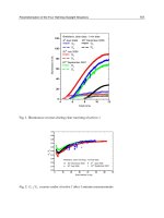
Figure 16 shows both the uplink and downlink call blocking probability, i.e. P
b,U
and P
b,D
.
Notice that the P
b,U
is always higher than the P
b,D
due to the asymmetric nature of multihop

transmission in CMCN that downlink transmission takes more channels from the central
microcell than uplink transmission. The channels used in the central microcells can be
reused in the other central microcells with minimum reuse distance without having to be
concerned about the co-channel interference constraint, because two-cell buffering is already
in place. The system capacity based on P
b,U
= 1% for MDCA with SCS and PCS are 15.3 and
16.3 Erlangs, respectively. With PCS-CR (channel reassignment), the capacity of MDCA is
increased by 0.4 Erlangs.
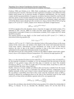
Figure 17 shows the average call blocking probabilities for FCA and DCA-WI for SCNs
(Chong & Leung, 2001), AFCA for CMCN (Li & Chong, 2006), MDCA with SCS, PCS and
PCS-CR. DCA-WI, known as DCA with interference information, is a distributed network-
based DCA scheme for SCNs. Under DCA-WI, each BS maintains an interference
information table and assigns channels according to the information provided by the table.
Only the P
b,U
for MDCA is shown because uplink transmission has lower capacity. At
P
b
,
U
= 1%, the system capacity for the FCA and DCA-WI are 4.5 Erlangs and 7.56 Erlangs,
respectively. AFCA with optimum channel combinations, UL(N
U,c
=22, N
U,v
=8) and
DL(N
D,c
=40, N

D,v
=5), can support 9.3 Erlangs. The MDCA with SCS, PCS, and PCS-CR
can support 15.3 Erlangs, 16.3 Erlangs and 16.7 Erlangs, respectively. As compared to DCA-
WI and AFCA, the improvements of MDCA with PCS-CR are 120.9% and 79.6%,
respectively.
10 12 14 16 18 20
10
-4
10
-3
10
-2
10
-1
10
0
Offered Traffic (Erlangs/Macrocell)
Call Blocking Probability
uplink, MDCA-SCS
downlink, MDCA-SCS
uplink, MDCA-PCS
downlink, MDCA-PCS
uplink, MDCA-PCS-CR
downlink, MDCA-PCS-CR


Fig. 16. Asymmetric capacity for uplink and downlink for CMCN using MDCA.
Channel Assignment in Multihop Cellular Networks

237

4 6 8 10 12 14 16
10
-3
10
-2
10
-1
10
0
Offered Traffic (Erlangs/Macrocell)
Call Blocking Probability
MDCA-SCS
MDCA-PCS
MDCA-PCS-CR
FCA (Erlang B)
DCA-WI
AFCA-UL(22, 8)-DL(40, 5)

Fig. 17. Capacity comparison with N=70.
Figure 18 shows the uplink blocking probabilities, P
b1
, P
b2
and P
b3
, for one-hop, two-hop and
three-hop calls respectively. As expected, P
b3
is generally higher than P
b2

, and P
b2
is higher
than P
b1
. The blocking probabilities for the three types of calls are lower for MDCA when
using the PCS strategy as opposed to the SCS strategy. This is because the PCS strategy
improves the channel availability and thus reduces the blocking probabilities of the three
types of calls. The PCS-CR is not included in Figure 18 because the purpose CR will simply
enhance the advantage of PCS by minimizing the effect of assigning a channel on the
channel availability of the whole system.
Figure 19 illustrates the performance of MDCA with a larger number of system channels,
when N=210. The Erlang B formula calculates that a SCN with N=210 can support only 20.3
Erlangs. The capacity for DCA-WI is 25.2 Erlangs. The capacity of CMCN with the optimum
AFCA channel combination AFCA-UL(72, 23)-DL(144, 11) is 54.4 Erlangs at P
b,U
=1%. The
MDCA using the SCS, PCS and PCS-CR strategies can support 61.5 Erlangs, 62.7 Erlangs
and 63.7 Erlangs, respectively. Therefore, the MDCA sustains its advantage over
conventional FCA, network-based DCA for SCNs and AFCA even for a large number of
system channels.
10 12 14 16 18 20
10
-4
10
-3
10
-2
10
-1

10
0
Offered Traffic (Erlangs/Macrocell)
Call Blocking Probabilities, P
b1
, P
b2
, P
b3
P
b1
, MDCA-SCS
P
b2
, MDCA-SCS
P
b3
, MDCA-SCS
P
b1
, MDCA-PCS
P
b2
, MDCA-PCS
P
b3
, MDCA-PCS

Fig. 18. Call blocking probability for different types of calls.
Cellular Networks - Positioning, Performance Analysis, Reliability

238
30 35 40 45 50 55 60 65 70
10
-4
10
-3
10
-2
10
-1
10
0
Offered Traffic (Erlangs/Macrocell)
Call Blocking Probability
AFCA-UL(72,23)-DL(144,11)
MDCA-SCS
MDCA-PCS
MDCA-PCS-CR
FCA (Erlang B)
DCA-WI

Fig. 19. Capacity comparison with N=210.
4.6.2 Simulation results with hot-spot traffic
First, as in (I & Chao, 1993), we adopted the same methodology to study the performance of
MDCA with the static hot-spot traffic. Two scenarios are simulated. As shown in Figure 20,
microcell 24 is chosen for the isolated one hot-spot model and microcells 2, 9, 17, 24, 31, 39, 46
are chosen to form the expressway model. First, each of the seven macrocells is initially loaded
with a fixed nominal amount of traffic, which would cause 1% blocking if the conventional
FCA were used. Next, we increase the traffic load in hot-spot microcells until the call

blocking in any hot-spot microcell reaches 1%. Then we can obtain the capacity values for
the hot-spot microcells areas.
With N = 70, each of the seven macrocells will be initially loaded at 4.46 Erlangs. In other
words, each microcell is loaded with 0.637 Erlangs. We increase the traffic load for hot-spot
cells, while keeping the traffic in non-hot-spot microcells at 0.637 Erlangs/Microcell. As
shown in Figure 21, for the isolated one hot-spot model, FCA, AFCA and MDCA supports
about 0.6 Erlangs, 9 Erlangs and 38 Erlangs per microcell, respectively. For the expressway
model, FCA, AFCA and MDCA supports about 0.6 Erlangs, 1 Erlangs and 6 Erlangs per
microcell, respectively. It can be seen that MDCA has a huge capacity to alleviate the
blocking in hot-spot cells.


6
8
10
11
13
14
16
18
19
20
21
22
23
25
26
27
28
29

30
32
34
35
37
38
40
41
42
43
44
47
48
BS
central
microcell
virtual
microcell
0
12
3
4
5
7
12
15
24
33
36
45

virtual
macrocell
46
39
31
9
17


Fig. 20. The simulated hot-spot traffic cell model.
Channel Assignment in Multihop Cellular Networks

239

0 5 10 15 20 25 30 35 40 45
10
-3
10
-2
10
-1
10
0
Offered Traffic for Hot-spot Microcells (Erlangs/Microcell)
Call Blocking Probability of Hot-spot Microcells
one hot-spot, MDCA-PCS-CR
one hot-spot, AFCA-UL(22,8)-DL(40,5)
expressway, MDCA-PCS-CR
expressway, AFCA-UL(22,8)-DL(40,5)
FCA (Erlang B)

Fig. 21. Capacity comparison with hot-spot traffic for N=70.
Significant capacity improvements of MDCA have been observed with a larger N, e.g. N =
210, with uniform and hop-spot traffic. Same conclusion can be drawn that MDCA has a
huge capacity to alleviate the blocking in hot-spot cells.
Finally, we investigate the performance of MDCA with a dynamic hot-spot traffic scenario
and compare MDCA with AFCA. Under this traffic model, 7 hot-spot microcells are
randomly selected from the 49 microcells shown in Figure 15. During the simulation, each
data point is obtained by simulating the channel assignment for a period of with 1000
million calls. This period is divided into 10 equal intervals. For each interval, 7 hot-spot
microcells are dynamically distributed over the 49-cell network by random selection. The
average call blocking statistics are collected from the 7 hot-spot microcells from each
interval. Notice that the selection of 7 hot-spot microcells is conducted for every interval and
no two intervals will use the identical set of hot-spot microcells. At the end of the



1 2 3 4 5 6 7 8 9 10
10
-4
10
-3
10
-2
10
-1
10
0
Offered Traffic for Hot-spot Microcells (Erlangs/Microcell)

Call Blocking Probability of Hot-spot Microcells
AFCA-UL(22,8)-DL(40,5)
MDCA-PCS-CR


Fig. 22. Capacity comparison with dynamic hot-spot traffic for N=70.
Cellular Networks - Positioning, Performance Analysis, Reliability

240
simulation, we calculate the average call blocking probability over the 10 intervals. The
traffic load in those non-hot-spot microcells is always 0.637 Erlangs/microcells according to
the static hot-spot traffic model.
Figure 22 shows the capacity results for AFCA and MDCA with the dynamic hot-spot traffic
scenario with N = 70 channels. MDCA and AFCA supports about 5.2 Erlangs and 1.0
Erlangs, respectively, at 1% call blocking. We can see that MDCA outperforms AFCA due to
its flexibility of handling dynamic traffic distribution.
5. Conclusion
Clustered multihop cellular network (CMCN) is proposed as a compliment to traditional
single-hop cellular networks (SCNs). A channel assignment, namely asymmetric fixed
channel assignment (AFCA) is further proposed for the use in CMCNs. To analyze its
performance, we have developed two multi-dimensional Markov chain models, including
an exact model and an approximated model. The approximated model results in lower
computational complexity and provides a good accuracy. Both models are validated
through computer simulations and they matched with each other closely. Results show that
the CMCN AFCA can increase the spectrum efficiency significantly. The system capacity
can be improved greatly by increasing the number of channels assigned to the central
microcell and decreasing the number of channels in the surrounding microcells. With
optimum channel combination in the CMCN, the capacity can be doubled as compared to
traditional SCNs.
We continued to investigate the feasibility of applying DCA scheme for MCN-type systems.

A multihop DCA (MDCA) scheme with two channel searching strategies is proposed for
clustered MCNs (CMCNs). Then, the computational complexity of the proposed MDCA
with the two channel searching strategies is analyzed. A channel reassignment procedure is
also investigated. Results show that MDCA can improve the system capacity greatly as
compared to FCA and DCA-WI for SCNs and AFCA for CMCNs. Furthermore, MDCA can
efficiently handle the hot-spot traffic.
In our analysis of fixed channel assignment scheme, we assumed that the MS population is
infinite and RSs can be always found when a two-hop or three-hop call is concerned. Note
that depending on the MS density, there would actually be an associated probability of
finding a RS. It will cause serious difficulties with the analysis to incorporate the associated
probability of finding a RS into the analytical models. Therefore, it has been left as part of
our future work.
6. Reference
Adachi, Tomoko, & Nakagawa, Masao, (1998). A Study on Channel Usage in a Cellular-Ad-
Hoc United Communication System for Operational Robots. IEICE Transactions on
Communications. Vol. E81-B, No. 7 (July 1998), pp. 1500-07.
Aggelou, George Neonakis, & Tafazolli, Rahim, (2001). On the Relaying Capability of Next
Generation Gsm Cellular Networks. IEEE Personal Communications. Vol. 8, No. 1
(February 2001), pp. 40-47.
Channel Assignment in Multihop Cellular Networks

241
Chong, P. H. J., & Leung, Cyril (2001). A Network-Based Dynamic Channel Assignment
Scheme for Tdma Cellular Systems. International Journal of Wireless Information
Networks. Vol. 8, No. 3 (July 2001), pp. 155-65.
Herber, S. Wilf. (1986). Algorithms and Complexity. 1st ed. Prentice-Hall, New Jersey, USA.
Hsu, Yu-Ching, & Lin, Ying-Dar, (2002). Multihop Cellular: A Novel Architecture for
Wireless Data Communications. Journal of Communications and Networks. Vol. 4, No.
1 (March 2002), pp. 30-39.
I, Chih-Lin, & Chao, Pi-Hui. (1993). Local Packing - Distributed Dynamic Channel

Allocation at Cellular Base Station. In Proceedings of IEEE GLOBECOM'93
(Houston, TX, USA, 29 November - 2 December 1993). 1, 293-301.
Kleinrock, Leonard. (1975). Queueing System 1st ed. John Wiley & Sons, New York.
Kudoh, E., & Adachi, F., (2005). Power and Frequency Efficient Wireless Multi-Hop Virtual
Cellular Concept. IEICE Transactions on Communications. Vol. E88B, No. 4 (Apr
2005), pp. 1613-21.
Li, Xue Jun, & Chong, P. H. J., (2008). Asymmetric Fca for Downlink and Uplink
Transmission in Clustered Multihop Cellular Network. Wireless Personal
Communications. Vol. 44, No. 4 (March 2008), pp. 341-60.
(2006). A Fixed Channel Assignment Scheme for Multihop Cellular Network. In
Proceedings of IEEE GLOBECOM'06 (San Francisco, CA, USA, 27 November - 1
December 2006). WLC 20-6, 1-5.
, (2010). Performance Analysis of Multihop Cellular Network with Fixed Channel
Assignment. Wireless Networks. Vol. 16, No. 2 (February 2010), pp. 511-26.
Lin, Yi-Bing, & Mak, Victor W., (1994). Eliminating the Boundary Effect of a Large-Scale
Personal Communication Service Network Simulation. ACM Transactions on
Modeling and Computer Simulation. Vol. 4, No. 2 (April 1994), pp. 165-90.
Lin, Ying-Dar, & Hsu, Yu-Ching. (2000). Multihop Cellular: A New Architecture for
Wireless Communications. In Proceedings of IEEE INFOCOM'00 (Tel Aviv, Israel,
26-30 March 2000). 3, 1273-82.
Liu, Yajian, et al., (2006). Integrated Radio Resource Allocation for Multihop Cellular
Networks with Fixed Relay Stations. IEEE Journal on Selected Areas in
Communications. Vol. 24, No. 11 (November 2006), pp. 2137-46.
Luo, Haiyun, et al. (2003). Ucan: A Unified Cellular and Ad-Hoc Network Architecture. In
Proceedings of ACM MOBICOM'03 (San Diego, CA, USA 14-19 September 2003). 1,
353-67.
Rappaport, Stephen S., & Hu, Lon-Rong, (1994). Microcellular Communication Systems with
Hierarchical Macrocell Overlays: Traffic Performance Models and Analysis.
Proceedings of The IEEE. Vol. 82, No. 9 (September 1994), pp. 1383-97.
Wu, Hongyi, et al. (2004). Managed Mobility: A Novel Concept in Integrated Wireless

Systems. In Proceedings of IEEE MASS'04 (Fort Lauderdale, FL, 24-27 October
2004). 1, 537-39.
, (2001). Integrated Cellular and Ad Hoc Relaying Systems: Icar. IEEE Journal on Selected
Areas in Communications. Vol. 19, No. 10 (October 2001), pp. 2105-15.
Cellular Networks - Positioning, Performance Analysis, Reliability

242
Yeung, Kwan L., & Nanda, S., (1996). Channel Management in Microcell/Macrocell Cellular
Radio Systems. IEEE Transactions on Vehicular Technology. Vol. 45, No. 4 (November
1996), pp. 601-12.
Yu, Jane Yang, & Chong, P. H. J., (2005). A Survey of Clustering Schemes for Mobile Ad Hoc
Networks. IEEE Communications Survey & Tutorials. Vol. 7, No. 1 (First Quarter
2005), pp. 32-48.


0
Mobility and QoS-Aware Service Management for
Cellular Networks
Omneya Issa
Communications Research Centre, Industry Canada
Canada
1. Introduction
As the technologies have evolved in cellular systems from 1G to 4G, the 4G system will
contain all the standards that earl ier gene rations have implemented. It is expected to provide
a comprehensive packet-based solution where multimedia applications and services can be
delivered to the subscriber on an anytime, anywhere basis with a satisfacto ry enoug h data
rate and advanced features, such as, quality of service (QoS), low latency, high mobility, etc.
Nevertheless, the 4G cellular system remains a wireless mobile environment, where resources
are not given and their availability is prone to dynamic changes. Hence, the basis for QoS
provisioning is to control the admission of new and handoff subscriber services in such a

way to avoid future detri ment perturb ation of already conne cted ones. This task becomes a
real challenge when service providers try to raise their profit, by maximizing the number of
connected subscribers, while meeting their customer QoS requirements.
The problem can be summarized in that the cellular network should meet the service
requirements of connected users using its underlying resources and features. These resources
must be managed in order to fulfill the QoS requirements of service connections while
maximizing the number of admitted subscribers. Furthermore, the solution(s) must account
for the environmental and mobility issues that influence the quality of RF channels, such as,
fading and interference. This is the role of service management in cellular networks.
In this chapter, we address service admission control and adaptation, which are the key
techniques of service management in mobile cellular networks characterized by restricted
resourc es and bandwidth fluctuation.
Several research efforts have been done for access control on wireless networks. The authors
of (Kelif & Coupechoux, 2009) developped an analytical study of mobility in cellular networks
and its impact on quality of service and outage probability. In (Kumar & Nanda, 1999),
the authors have proposed a burst-mode packet access scheme in which high data rates are
assigned to mobiles for s hort burst durations, based on load and interference measurements.
It covers burst-mode only assuming that mobiles have only right to one service.
The authors of (Comaniciu et al., 2000) have proposed an admission control for an integrated
voice/www sessions CDMA system based on average load measurements. It assumes that
all data users have the same bit error rate (BER) requirements. A single cell environment is
modeled and no interference is considered. In (Kwon et al., 2003), authors have presented
a QoS provisioning framework where a distributed admission control algorithm guarantees
the upper bound of a redefined QoS parameter called cell overload probability. Only a s ingle
1
Mobility and QoS-Aware Service Management
for Cellular Networks
10
class has been investigated; however, interference and fading are not taken into consideration.
Also, the authors of (Kastro et al., 2010) proposed a model combining the information about

the customer demographics and usage behavior together with call information, yielding to a
customer-oriented resource management strategy for cellular networks to be applied during
call initiation, handoff and allocation of mobile base stations. Although the model addressed
well customer satisfaction within the studied cell, it did not consider interference to other
cells.
The authors of (Aissa et al., 2004) proposed a way of predicting resource utilization increase,
which is the total received/transmitted power, that would result when accepting an incoming
call. Their admission control involves comparing the approximate predicted power with a
threshold; this threshold is obtained by determining (offline) the permissible loading in a
cell in a static scenario. However, the interference of other cells is not considered in the
static scenario and no service adaptation is studied. In (Nasser & Hassanein, 2004; 2006),
despite the fact that the authors have proposed a prioritized call admission control scheme and
bandwidth adaptation algorithm for multimedia calls in cellular networks, their framework
only supported a single class and only bandwidth is considered in adaptation, which is not
tolerated by some multimedia services, such as, voice calls. They did not consider neighbor
cell interference as well.
Other research efforts analyzed the soft handoff failure due to insufficient system capacity as
done in this chapter. As an example, IS-95 and cdma2000 are compared with respect to the
soft handoff performance in terms of outage, new call and handoff call blocking in (Homnan
et al., 2000). In (Him & Koo, 2005), the call attempts of new and handoff voice/data calls are
blocked if there is no channel available, and a soft handoff blocking probability is derived as
well.
In what concerns the admission policies of handoff calls with respect to new calls, some
schemes, such as the ones proposed in (Cheng & Zhuang, 2002; Kulavaratharasah & Aghvami ,
1999), deploy a guard channel to reserve a fixed percentage of the BS’s capacity for handoff
users. Other schemes, called nonprioritized schemes in (Chang & Chen, 2006; Das et al.,
2000), handle handoff calls exactly the same way they do with the new calls. Although these
approaches are not specially designed, they can be adapted to 3G+ networks as it was briefly
represented in (Issa & Gregoire, 2006) and will be discussed in this chapter.
The above survey has compared state-of-the art admission control proposals, highlighting the

main factors of decision making, advantages and weaknesses of different approaches. This
leads to pointing out that important challenges pertaining to the wireless environment are
yet to be addressed. Therefore, this chapter proposes a strategy that ac counts for most of
these challenges, such as, cell loading, inter-cell and intra-cell interference, soft handoff as
well as QoS requirements in making admission decisions. The strategy also considers the fact
that, nowadays, mobile devices are not just restricted to cellular phones; instead, they became
small workstations that allow for several simultaneous services per user connection. Factors
such as service tolerance for degradation and QoS parameters allowed to be degraded are
also exploited. The chapter is organized as follows: in sections 2 and 3 we describe the design
details of our approach followed by the d es ign evaluation in section 4, then we summarize
the benefits of the proposal and present future work in section 5.
2. Admission control
Our scheme of service admission on either forward or reverse links is done by measuring
the total receive d or transmitted power at the base station and calculating the available
244
Cellular Networks - Positioning, Performance Analysis, Reliability
class has been investigated; however, interference and fading are not taken into consideration.
Also, the authors of (Kastro et al., 2010) proposed a model combining the information about
the customer demographics and usage behavior together with call information, yielding to a
customer-oriented resource management strategy for cellular networks to be applied during
call initiation, handoff and allocation of mobile base stations. Although the model addressed
well customer satisfaction within the studied cell, it did not consider interference to other
cells.
The authors of (Aissa et al., 2004) proposed a way of predicting resource utilization increase,
which is the total received/transmitted power, that would result when accepting an incoming
call. Their admission control involves comparing the approximate predicted power with a
threshold; this threshold is obtained by determining (offline) the permissible loading in a
cell in a static scenario. However, the interference of other cells is not considered in the
static scenario and no service adaptation is studied. In (Nasser & Hassanein, 2004; 2006),
despite the fact that the authors have proposed a prioritized call admission control scheme and

bandwidth adaptation algorithm for multimedia calls in cellular networks, their framework
only supported a single class and only bandwidth is considered in adaptation, which is not
tolerated by some multimedia services, such as, voice calls. They did not consider neighbor
cell interference as well.
Other research efforts analyzed the soft handoff failure due to insufficient system capacity as
done in this chapter. As an example, IS-95 and cdma2000 are compared with respect to the
soft handoff performance in terms of outage, new call and handoff call blocking in (Homnan
et al., 2000). In (Him & Koo, 2005), the call attempts of new and handoff voice/data calls are
blocked if there is no channel available, and a soft handoff blocking probability is derived as
well.
In what concerns the admission policies of handoff calls with respect to new calls, some
schemes, such as the ones proposed in (Cheng & Zhuang, 2002; Kulavaratharasah & Aghvami ,
1999), deploy a guard channel to reserve a fixed percentage of the BS’s capacity for handoff
users. Other schemes, called nonprioritized schemes in (Chang & Chen, 2006; Das et al.,
2000), handle handoff calls exactly the same way they do with the new calls. Although these
approaches are not specially designed, they can be adapted to 3G+ networks as it was briefly
represented in (Issa & Gregoire, 2006) and will be discussed in this chapter.
The above survey has compared state-of-the art admission control proposals, highlighting the
main factors of decision making, advantages and weaknesses of different approaches. This
leads to pointing out that important challenges pertaining to the wireless environment are
yet to be addressed. Therefore, this chapter proposes a strategy that ac counts for most of
these challenges, such as, cell loading, inter-cell and intra-cell interference, soft handoff as
well as QoS requirements in making admission decisions. The strategy also considers the fact
that, nowadays, mobile devices are not just restricted to cellular phones; instead, they became
small workstations that allow for several simultaneous services per user connection. Factors
such as service tolerance for degradation and QoS parameters allowed to be degraded are
also exploited. The chapter is organized as follows: in sections 2 and 3 we describe the design
details of our approach followed by the d es ign evaluation in section 4, then we summarize
the benefits of the proposal and present future work in section 5.
2. Admission control

Our scheme of service admission on either for ward or reverse links is done by measuring
the total receive d or transmitted power at the base station and calculating the available
capacity according to QoS constraints, interference measurements and fading information
gathered from Mobile stations (MSs) in the neighbouring cells. The advantage of b uilding
our admission control scheme on power constraints is that it incorporates both bandwidth
and BER, represented in target Signal to interference ratio (SIR), since both band w idth and
SIR affect the required channel power and are important in guaranteeing QoS especially
in a wireless mobile environment. In addition to power constraints, our admission control
follows a policy-based criterion by giving the handoff services priority over the new service
connections. In fact, soft handoff attempts should be considered differently from new call
attempts because the rejection of handoff attempts from other cells could cause call dropping.
Fig. 1. Admission control scheme
Fig. 1 shows the admission control process. When a new service is required, the base station
(BS) admission control (AC) module calculates the required capacity in terms of channel
245
Mobility and QoS-Aware Service Management for Cellular Networks
power needed, then checks the available capacity taking into account the current service load,
the mobile transmit power, the interference of other cells and the interference to neighbour
cells. If the available capacity can not cover the initial requirements of the incoming services,
the admission control scheme appeals to a degradation procedure for connected services.
However, if the degr adation process can not recover the needed capacity, the admission
control module adjusts the requirements of the incoming services (only services requiring
minimum throughput). However, when such adjustment is not enough, it start s rejecting new
service requests. Service degradation is discussed in section 3.
We start by describing the verification of load and interference done at beginning of the
admission control procedure before appealing to service degradation. The basic idea in
resource estimation is actually the same for both uplink (reverse) and downlink (forward).
2.1 Uplink
Assuming one BS per cell, this capacity validation procedure is done as follows on the uplink:
Pt

K
=
∑
j
P
j,K
+ Other_Cell_Inter f erence + No, (1)
where Pt
K
is the total received power by the BS in cell K, P
j,K
is the received power at cell K
from MS
j
and No is the background noise. As in (Kumar & Nanda, 1999), P
j,K
can be written
as a function of SIR, i.e. the received ratio of signal bit energy to noise power spectral d ensity
(Eb/No)
j,K
for MS
j
in cell K divided by its processing gain G
j
,
P
j,K
=
1
G

j
Pt
K

Eb
No

j,K
, G
j
=
W
R
j
, (2)
W is the spreading bandwidth and R
j
represents the transmission rate of MS
j
. Including SIR
in capacity measurements is very important since 3G+ network is interference limited.
2.1.1 Interference calculation
The other interference in cell K caused by neighbouring cells can be presented in an average
sense as a fraction of the in-cell load (Gilhousen et al., 1991), on condition that the load is
uniform across all cells. We relaxed this condition to the case where the load in different cells
is different, but the average load over all cells is kept fixed to some value by the base station
controller (B SC). So (1) can be rewritten as
Pt
K
=

(
1 + η
K
)
·
∑
j
P
j,K
+ No
= Pt
K
·


∑
j
1
G
j

Eb
No

j,K


·
(
1 + η

K
)
+
No,
(3)
where the other cell interference factor η
K
is de fined as in (Kim et al., 2003)
η
K
=
∑
i=K

1
M
i
M
i
∑
x=1
η(x)

, (4)
246
Cellular Networks - Positioning, Performance Analysis, Reliability
power needed, then checks the available capacity taking into account the current service load,
the mobile transmit power, the interference of other cells and the interference to neighbour
cells. If the available capacity can not cover the initial requirements of the incoming services,
the admission control scheme appeals to a degradation procedure for connected services.

However, if the degr adation process can not recover the needed capacity, the admission
control module adjusts the requirements of the incoming services (only services requiring
minimum throughput). However, when such adjustment is not enough, it start s rejecting new
service requests. Service degradation is discussed in section 3.
We start by describing the verification of load and interference done at beginning of the
admission control procedure before appealing to service degradation. The basic idea in
resource estimation is actually the same for both uplink (reverse) and downlink (forward).
2.1 Uplink
Assuming one BS per cell, this capacity validation procedure is done as follows on the uplink:
Pt
K
=
∑
j
P
j,K
+ Other_Cell_Inter f erence + No, (1)
where Pt
K
is the total received power by the BS in cell K, P
j,K
is the received power at cell K
from MS
j
and No is the background noise. As in (Kumar & Nanda, 1999), P
j,K
can be written
as a function of SIR, i.e. the received ratio of signal bit energy to noise power spectral d ensity
(Eb/No)
j,K

for MS
j
in cell K divided by its processing gain G
j
,
P
j,K
=
1
G
j
Pt
K

Eb
No

j,K
, G
j
=
W
R
j
, (2)
W is the spreading bandwidth and R
j
represents the transmission rate of MS
j
. Including SIR

in capacity measurements is very important since 3G+ network is interference limited.
2.1.1 Interference calculation
The other interference in cell K caused by neighbouring cells can be presented in an average
sense as a fraction of the in-cell load (Gilhousen et al., 1991), on condition that the load is
uniform across all cells. We relaxed this condition to the case where the load in different cells
is different, but the average load over all cells is kept fixed to some value by the base station
controller (B SC). So (1) can be rewritten as
Pt
K
=
(
1 + η
K
)
·
∑
j
P
j,K
+ No
= Pt
K
·


∑
j
1
G
j


Eb
No

j,K


·
(
1 + η
K
)
+
No,
(3)
where the other cell interference factor η
K
is de fined as in (Kim et al., 2003)
η
K
=
∑
i=K

1
M
i
M
i
∑

x=1
η(x)

, (4)
M
i
is the number of M Ss in cell i and η(x) is calcul ated as
η
(x)=
ρ
K
(i, x)L
K
(i, x)
ρ
i
(i, x)L
i
(i, x)
, (5)
where ρ
K
(i, x) is the fast (Rayleigh) fading and is given by
ρ
K
(i, x)=
P
∑
p=1
g

2
K,x
(i),p
, (6)
with g
2
K,x
(i),p
is the p
th
path gain between BS
K
and MS
x
in cell i, and L
K
(i, x) presents slow
fading which is modeled as
L
K
(i, x)=r
−δ
K,x
(i)
· 10
ξ
K,x(i)
/10
, (7)
where the signal between BS

K
and MS
x
in cell i ex per iences an attenuation by the δth power
of the distance r
K,x(i)
between BS
K
and MS
x
and log-normal shadowing (ξ is a zero-normal
variant with standard variation σ).
The uplink capacity is directly affected by the noise rise generated by users in the uplink. The
noise rise N
r
is the increase in noise compared to the noise floor of the cell; thus:
N
r
=
Pt
K
No
, (8)
The concept of noise rise means that infinite noise rise must be considered when the load is
100% (e.g. the pole capacity). Hence, N
r
can be written as a function the cell uplink load C
U
;
when C

U
is close to unity, the noise rise approaches infinity as shown in (9):
N
r
=
1
1 − C
U
, (9)
From (8) , the C
U
can be written in function of the total received power as follows:
C
U
=
Pt
K
− No
Pt
K
, (10)
Using (3),
C
U
=
(
1 + η
K
)
·

∑
j
P
j,K
Pt
K
, (11)
Recall that from (2),
P
j,K
Pt
K
=
R
j
W

Eb
No

j,K
, (12)
So (11) becomes:
C
U
=
(
1 + η
K
)

·
∑
j
R
j
W

Eb
No

j,K
, (13)
(13) assumes only one channel per MS. To extend it to the case, as for wideband CDMA, where
an MS can have several channels with different target SIR’s, data rates and activity factors, (13)
can be written as
C
U
=


1
W
∑
j
N
j
∑
n=1
R
n,j,K


Eb
No

n,j,K
a
n,j,K


·
(
1+η
K
)
, (14)
247
Mobility and QoS-Aware Service Management for Cellular Networks
where N
j
is the number of channels of MS
j
, and (Eb/No)
n,j,K
and a
n,j,K
are the received Eb/No
and the activity factor for service of channel n of MS
j
in cell K respectively.
So the admission condition for accepting the uplink connection(s) of MS

i
in cell K is
(
1 + η
K
)
W


∑
j=i
N
j
∑
n=1
R
n,j,K

Eb
No

n,j,K
a
n,j,K


+
(
1 + η
K

)
W

N
i
∑
n=1
R
n,i,K

Eb
No

n,i,K
a
n,i,K

≤ Th
U
,
(15)
where N
i
is the number of channels of MS
i
, (Eb/No)
n,i,K
is the required Eb/No (SIR) for
channel n o f MS
i

in cell K and η
K
is computed by (4-7). Theoretically, Th
U
is equal to 1, which
is the pole capacity. However, an operator restricts the uplink load to a certain noise rise,
hence, practically Th
U
is kept below unity.
2.2 Downlink
The downlink cell capacity follows the same logic as the uplink. The total base station
transmit power, Ptx_tot
K
, is estimated. It is the sum of individual transmit powers required
for downlink connections of MSs in a cell as shown below.
Ptx_tot
K
=
∑
j
Ptx
j,K
, (16)
where Ptx
j,K
is the downlink power required for MSj in cell K, assuming only one s ervice per
mobile. Ptx
j,K
is given by (Sipila et al., 2000):
Ptx

j,K
=
R
j
W

Eb
No

j,K
·

(
1 − f
)
Ptx_tot
K
+ η
j
· Ptx_tot
K
+ No · L
K,j

, (17)
where L
K,j
is the path loss from base station K to MS
j
and f is the orthogonality factor

modeling the intracell interference from non-orthogonal codes of other MSs, using f =1 for
fully orthogonal codes and 0 as not or thogonal. Note that the orthogonality factor f depends
on the codes used for users inside a cell, and even if these codes are perfectly orthogonal, there
is always some degree of interference between the signals of mobiles of the same cell due to
multi-path. Delayed copies received from a multipath fading are not orthogonal any more
and cause multipath fading interference, which is modeled as a factor of the total base station
transmit power. For s implicity, we do not consider the orthogonality factor of each code; we
take f as the average orthogonality factor in the cell. η
j
is the other-cell-to-own-cell received
power ratio (inter-cell interference) for M S
j
modeled as a factor of the total downlink power
and calculated as follows:
η
j
=
∑
i=K
ρ
K,j
L
K,j
ρ
i,j
L
i,j
, (18)
where ρ
K,j

and L
K,j
are the fast and slow (path loss) fading from the serving base station K to
MS
j
and ρ
i,j
and L
i,j
are the fast and slow (path l oss) fading from another base station i to MS
j
respectively.
The other-to-own-cell interference on the downlink depends on mobile location and,
therefore, is different for each mobile. However, the estimation of the downlink transmission
power should be on average basis and not on the maximum transmission power at the cell
248
Cellular Networks - Positioning, Performance Analysis, Reliability
where N
j
is the number of channels of MS
j
, and (Eb/No)
n,j,K
and a
n,j,K
are the received Eb/No
and the activity factor for service of channel n of MS
j
in cell K respectively.
So the admission condition for accepting the uplink connection(s) of MS

i
in cell K is
(
1 + η
K
)
W


∑
j=i
N
j
∑
n=1
R
n,j,K

Eb
No

n,j,K
a
n,j,K


+
(
1 + η
K

)
W

N
i
∑
n=1
R
n,i,K

Eb
No

n,i,K
a
n,i,K

≤ Th
U
,
(15)
where N
i
is the number of channels of MS
i
, (Eb/No)
n,i,K
is the required Eb/No (SIR) for
channel n o f MS
i

in cell K and η
K
is computed by (4-7). Theoretically, Th
U
is equal to 1, which
is the pole capacity. However, an operator restricts the uplink load to a certain noise rise,
hence, practically Th
U
is kept below unity.
2.2 Downlink
The downlink cell capacity follows the same logic as the uplink. The total base station
transmit power, Ptx_tot
K
, is estimated. It is the sum of individual transmit powers required
for downlink connections of MSs in a cell as shown below.
Ptx_tot
K
=
∑
j
Ptx
j,K
, (16)
where Ptx
j,K
is the downlink power required for MSj in cell K, assuming only one s ervice per
mobile. Ptx
j,K
is given by (Sipila et al., 2000):
Ptx

j,K
=
R
j
W

Eb
No

j,K
·

(
1 − f
)
Ptx_tot
K
+ η
j
· Ptx_tot
K
+ No · L
K,j

, (17)
where L
K,j
is the path loss from base station K to MS
j
and f is the orthogonality factor

modeling the intracell interference from non-orthogonal codes of other MSs, using f =1 for
fully orthogonal codes and 0 as not or thogonal. Note that the orthogonality factor f depends
on the codes used for users inside a cell, and even if these codes are perfectly orthogonal, there
is always some degree of interference between the signals of mobiles of the same cell due to
multi-path. Delayed copies received from a multipath fading are not orthogonal any more
and cause multipath fading interference, which is modeled as a factor of the total base station
transmit power. For s implicity, we do not consider the orthogonality factor of each code; we
take f as the average orthogonality factor in the cell. η
j
is the other-cell-to-own-cell received
power ratio (inter-cell interference) for MS
j
modeled as a factor of the total downlink power
and calculated as follows:
η
j
=
∑
i=K
ρ
K,j
L
K,j
ρ
i,j
L
i,j
, (18)
where ρ
K,j

and L
K,j
are the fast and slow (path loss) fading from the serving base station K to
MS
j
and ρ
i,j
and L
i,j
are the fast and slow (path l oss) fading from another base station i to MS
j
respectively.
The other-to-own-cell interference on the downlink depends on mobile location and,
therefore, is different for each mobile. However, the estimation of the downlink transmission
power should be on average basis and not on the maximum transmission power at the cell
edge. The average transmission power per mobile is determined by considering the user at an
average location in the cell. Thus, we may let η be the average other-to-own cell interference
seen by the mobile as in (Sipila et al., 2000):
η
=
1
J
∑
j
η
j
, (19)
where J is the number of MSs served by the base station.
By summing up Ptx
j,K

over the number of MSs, Ptx_tot
K
can be derived as in (20). Note that
in this estimation the soft handover must be included. thus, j must include the soft handover
connections, which are modeled as additional connections in the cell, as well.
Ptx_tot
K
=
No
∑
j
R
j
W

Eb
No

j,K
L
K,j
1 −
∑
j
R
j
W

Eb
No


j,K
·
((
1 − f
)
+
η
)
, (20)
Using the same reasoning on the noise rise as for the uplink, we can define the cell downlink
load C
D
as follows (Sipila et al., 2000):
C
D
=
∑
j
R
j
W

Eb
No

j,K
·
((
1 − f

)
+
η
)
, (21)
When C
D
is close to 1, the base station transmit po w er approaches infinity. To extend (21) so
that an MS can have several channels with different activity factors, w e obtain the admission
condition for the downlink connection of MSi by:
(
1− f +η
)
W


∑
j=i
N
j
∑
n=1
R
n,j,K

Eb
No

n,j,K
a

n,j,K


+
(
1− f +η
)
W

N
i
∑
n=1
R
n,i,K

Eb
No

n,i,K
a
n,i,K

≤Th
D
,
(22)
Theoretically, Th
D
is equal to unity, which is called the pole capacity. However, lower Th

D
values will be tested to limit the noise rise. Note that in case of no orthogonality ( f = 0), (22)
becomes similar to the uplink case.
2.3 Reverse connections and soft handoff
In reverse connections, a MS can have more than one leg in soft handoff. So, in addition to
the procedure proposed above, to account for soft handoff, the following conditions must be
satisfi ed:
• j in (15) is summed over the set of MSs that have cell K in their active set.
• (15) must be satisfied for each soft handoff leg of MS
i
.
• Since adjacent-cell interference is critical in deciding for the admission of reverse
connections, it is necessary to evaluate the interference at the non active cells caused by
the admission of the reverse connection. So, interference constraints at neighbour cells
that are not in the active or candidate set of MS
i
should be satisfied.
249
Mobility and QoS-Aware Service Management for Cellular Networks
Pilot strength information received at MS
i
for cells in its neighbour list can indicate to BS the
interference levels that will be seen at its neighbour BSs due to transmissions from MS
i
. The
MS reports pilot strength information for cells in its neighbour list in the Paging Channel.
So, to avoid producing excessive interference at a neighbour cell NC, we constrain the path
loss difference between the strongest active and strongest non-active pilots to a minimum ∆
(Kumar & Nanda, 1999) such that
PS

0
− PS
NC
≥ ∆, (23)
PS
0
= max
K
(PS
iK
), K ∈ AS,
PS
NC
= max
K
(PS
iK
), K /∈ AS and K ∈ NS,
where PS
iK
is the pilot strength reported by MS
i
from cell K, AS is the set of active and
candidate pilots and NS is the set of neighbour pilots. PS
0
is the strength of the strongest
active pilot and PS
NC
is the strength of the strongest non-active pilot.
2.4 User equipment transmi t power

Another factor that must be taken into account, is the limited transmission power available at
the mobile stations. Here, we do not model battery lives, however, we check if the transmit
power of the mobile station, required to meet the uplink target Eb/No, does not exceed the
maximum mobile transmit power. As indicated in Fig.1, after the uplink cell load is checked,
the required mobile transmit power is verified with respect to its maximum. The required
mobile transmit power Ptx
MS
i,K
of MSi can be computed as follows (Sipila et al., 2000):
Ptx
MS
i,K
=
No

N
i
∑
n=1
R
n,i,K

Eb
No

n,i,K
a
n,i,K

L

i,K
1 − C
U
, (24)
where N
i
is the number of uplink channels of M S
i
. A mobile station, which is not able to
transmit with the required amount of power to meet the required Eb/No due to maximum
power limitations is not admitted (blocked). Note that incoming service requests can be
blocked either because of noise rise limits (equations (15) and (22)) or in case of limited mobile
transmit power. It is worth noting that the limitation of total base station power is already
considered by applying lower values of the threshold Th
D
in (22).
2.5 Recalculation of admitted load
A new channel can be assigned by sending a Channel Assignment Message with Service
Response Message to MS if all the above conditions are met. However, if all the conditions
are satisfied except the uplink condition (15) or the downlink one (22), the admission module
asks the Degradation module to try to acquire the capacity left to satisfy the required one.
In order to c ompute the capacity required from the Degr adation module , (15) and (22) are
interpreted in terms of the available capacity. The available capacities C
av
U
and C
av
D
for
accepting services on the uplink (U) and downlink (D) respectively can be given by:

C
av
U
=
W·Th
U
(
1+η
K
)
−

∑
i
N
i
∑
n=1
R
U
n,i,K

Eb
No

U
n,i,K
a
U
n,i,K


, (25)
250
Cellular Networks - Positioning, Performance Analysis, Reliability
Pilot strength information received at MS
i
for cells in its neighbour list can indicate to BS the
interference levels that will be seen at its neighbour BSs due to transmissions from MS
i
. The
MS reports pilot strength information for cells in its neighbour list in the Paging Channel.
So, to avoid producing excessive interference at a neighbour cell NC, we constrain the path
loss difference between the strongest active and strongest non-active pilots to a minimum ∆
(Kumar & Nanda, 1999) such that
PS
0
− PS
NC
≥ ∆, (23)
PS
0
= max
K
(PS
iK
), K ∈ AS,
PS
NC
= max
K

(PS
iK
), K /∈ AS and K ∈ NS,
where PS
iK
is the pilot strength reported by MS
i
from cell K, AS is the set of active and
candidate pilots and NS is the set of neighbour pilots. PS
0
is the strength of the strongest
active pilot and PS
NC
is the strength of the strongest non-active pilot.
2.4 User equipment transmi t power
Another factor that must be taken into account, is the limited transmission power available at
the mobile stations. Here, we do not model battery lives, however, we check if the transmit
power of the mobile station, required to meet the uplink target Eb/No, does not exceed the
maximum mobile transmit power. As indicated in Fig.1, after the uplink cell load is checked,
the required mobile transmit power is verified with respect to its maximum. The required
mobile transmit power Ptx
MS
i,K
of MSi can be computed as follows (Sipila et al., 2000):
Ptx
MS
i,K
=
No


N
i
∑
n=1
R
n,i,K

Eb
No

n,i,K
a
n,i,K

L
i,K
1 − C
U
, (24)
where N
i
is the number of uplink channels of M S
i
. A mobile station, which is not able to
transmit with the required amount of power to meet the required Eb/No due to maximum
power limitations is not admitted (blocked). Note that incoming service requests can be
blocked either because of noise rise limits (equations (15) and (22)) or in case of limited mobile
transmit power. It is worth noting that the limitation of total base station power is already
considered by applying lower values of the threshold Th
D

in (22).
2.5 Recalculation of admitted load
A new channel can be assigned by sending a Channel Assignment Message with Service
Response Message to MS if all the above conditions are met. However, if all the conditions
are satisfied except the uplink condition (15) or the downlink one (22), the admission module
asks the Degradation module to try to acquire the capacity left to satisfy the required one.
In order to c ompute the capacity required from the Degr adation module , (15) and (22) are
interpreted in terms of the available capacity. The available capacities C
av
U
and C
av
D
for
accepting services on the uplink (U) and downlink (D) respectively can be given by:
C
av
U
=
W·Th
U
(
1+η
K
)
−

∑
i
N

i
∑
n=1
R
U
n,i,K

Eb
No

U
n,i,K
a
U
n,i,K

, (25)
C
av
D
=
W · Th
D
((
1 − f
)
+
η
)
−


∑
i
N
i
∑
n=1
R
D
n,i,K

Eb
No

D
n,i,K
a
D
n,i,K

, (26)
where i is summed over the set of existing (already connected) MSs.
Since the first term in (25) and (26) does not depend on the service requirements, for simplicity,
we define a variable C that accou nts for the second term that varies according to services;
it will be referred to as ’service capacity’. Thus, the total required service capacity for
new/handoff requests, for uplink and downlink, can be written as:
C
tot_req
U/D
=



∑
j
N
j
∑
n=1
R
(U/D)
n,j,K

Eb
No

(U/D)
n,j,K
a
(U/D)
n,j,K


, (27)
where j is summed over the set of the new/handoff MSs and N
j
is the number of services on
either the uplink or the downlink. If C
tot_req
U/D
can not be satisfied by the available capacity,

the admission control appeals service degradation with the uplink and downlink d emanded
service capacities, C
d
U
and C
d
D
respectively. The demanded capacity is the difference between
the required capacity and the avai lable one:
C
d
= C
tot_req
− C
av
,
C
d
U
=


∑
j
N
j
∑
n=1
R
U

n,i,K

Eb
No

U
n,i,K
a
U
n,i,K


−
W·Th
U
(
1+ η
K
)
,
C
d
D
=


∑
j
N
j

∑
n=1
R
D
n,i,K

Eb
No

D
n,i,K
a
D
n,i,K


−
W · Th
D
((
1 − f
)
+
η
)
,
(28)
where j is summed over the set of existing MSs as well as the new/handoff ones.
If the capacity recovered by service degradation, C
recovered

, can provide the demanded
capacity, the service reques ts are accepted. However, to account for a worst case scenario
where the Degradation module cannot deliver the demanded capacity, the AC module, in
order to maximize the number of admitted services, recalculates the required capacity by
trying to decrease the accepted load of new/handoff minimum throughput services only,
since bounded delay services such as voice and video cannot tolerate such process. However,
the accepted load of each minimum throughput service is reduced, if possible, by an equal
share of unacquired capacity. In other words, each minimum throughput service will have an
equal share of the total now available c apacity (C
av
+ C
recovered
− C
reqBD
) with respect to the
required capacity of all the new/handoff minimum throughput services. C
reqBD
is the capacity
required for bounded delay new/handoff services. Note that the service requirements are not
decreased below the QoS limits, C
min
, indicated in its QoS profile. Thus, the accepted capacity
of service n is the greater of two values, its minimum required capacity and its share of the
total available capacity:
C
n_accepted
= max(C
n_min
, C
n_req

· (C
av
+ C
recovered
− C
reqBD
)/
N
∑
j=1
C
j_req
), (29)
where C
n
= R
n
(Eb/No)
n
a
n
, where R
n
and (Eb/No)
n
are the rate and the SIR of the channel
needed for service n respectively, and a
n
is the service activity factor. N is the number of
251

Mobility and QoS-Aware Service Management for Cellular Networks
new/handoff minimum throughput services. It will be seen in the next sectio n that the load
of minimum throughput services is decreased by adjusting their rate R.
It can happen, even when reducing the capacity of minimum throughput services, that the
accepted capacity exceeds available plus recovered capacities because we do not reduce the
service capacity below the limits of its QoS profile. So the last possible course of action
is to reject requests, as in Fig.1. We begin by rejecting new service requests since forced
termination of handoff services has significant negative effect on the user’s perception of
network reliability, and, therefore, affect subscribers’ expectation.
It is worth noting that the admission control scheme is simple to apply and has a low
computation time. The time complexity for calculating conditions (15) and (22) is of order
O
((Nc + 1)M) and the one for reducing the accepted load of new/handoff minimum
throughput services is of order O
(N
minT
) where Nc in the number of neighbour cells, M
in the average number of MSs per cell and N
minT
is the number of new/handoff minimum
throughput services. So the time complexity of our admission module is of order O
((Nc +
1)M + N
minT
), that is O(M) since Nc is limited to a few cells. In fact, the complexity of the
proposed approach is considered low with respect to the inclusion of a realistic interference
computing. Other complex approaches adopt a global call admission control where the actual
interference should be computed between all cells; their computational complexity is of order
of O
(N

2
) where N is the number of cells in the network. On the other hand, more simplistic
admission control algorithms simply consider the calls currently active in the intended cell in
order to accept or reject a new call. The inter-cell interference is either neglected or sometimes
considered as a constant factor. These algorithms usually have the lowest computational
complexity of O
(1), which is an optimal complexity, however, at the cost of not considering
realistic conditions.
3. Degradation and improvement
The problem of high new call blocking and handoff dropping can be partially solved by QoS
adaptation (degradation) which is much more bearable to users than a forced termination
of their services. The improvement module is important for deciding the appropriate
distribution of resources freed by terminating and ongoing services. Also, the admission
control needs this module in order to make room for admitting new and handoff connections.
In (Lee et al., 2000) authors have proposed an adaptive re source allocation mechanism
that allocates connection resources for incoming calls utilizing bandwidth degradation and
compensation. Also (Kwon et al., 2003) have proposed a bandwidth adaptation algorithm
which seeks to minimize a redefined QoS parameter called cell overload probability. Both
adaptation fr ameworks only take mobility into consideration; they do not account for fading
and interference. Both approaches consider only the transmission rate as the only parameter to
degrade. Moreover, all calls that exceed their average or minimum bandwidth are degraded to
their average or minimum bandwidth respectively. This requires a large number of s ignalling
messages.
3.1 Limiting signalling overhead
Service degradation/improvement implies changing resources assignment. This can be a time
and bandwidth-consuming process, because the number of degraded/ improved services
increases the amount of required signalling messages respectively. So we have decided to
limit the number of degraded/improved services by selecting only MSs located in a certain
zone of the cell.
252

Cellular Networks - Positioning, Performance Analysis, Reliability
new/handoff minimum throughput services. It will be seen in the next sectio n that the load
of minimum throughput services is decreased by adjusting their rate R.
It can happen, even when reducing the capacity of minimum throughput services, that the
accepted capacity exceeds available plus recovered capacities because we do not reduce the
service capacity below the limits of its QoS profile. So the last possible course of action
is to reject requests, as in Fig.1. We begin by rejecting new service requests since forced
termination of handoff services has significant negative effect on the user’s perception of
network reliability, and, therefore, affect subscribers’ expectation.
It is worth noting that the admission control scheme is simple to apply and has a low
computation time. The time complexity for calculating conditions (15) and (22) is of order
O
((Nc + 1)M) and the one for reducing the accepted load of new/handoff minimum
throughput services is of order O
(N
minT
) where Nc in the number of neighbour cells, M
in the average number of MSs per cell and N
minT
is the number of new/handoff minimum
throughput services. So the time complexity of our admission module is of order O
((Nc +
1)M + N
minT
), that is O(M) since Nc is limited to a few cells. In fact, the complexity of the
proposed approach is considered low with respect to the inclusion of a realistic interference
computing. Other complex approaches adopt a global call admission control where the actual
interference should be computed between all cells; their computational complexity is of order
of O
(N

2
) where N is the number of cells in the network. On the other hand, more simplistic
admission control algorithms simply consider the calls currently active in the intended cell in
order to accept or reject a new call. The inter-cell interference is either neglected or sometimes
considered as a constant factor. These algorithms usually have the lowest computational
complexity of O
(1), which is an optimal complexity, however, at the cost of not considering
realistic conditions.
3. Degradation and improvement
The problem of high new call blocking and handoff dropping can be partially solved by QoS
adaptation (degradation) which is much more bearable to users than a forced termination
of their services. The improvement module is important for deciding the appropriate
distribution of resources freed by terminating and ongoing services. Also, the admission
control needs this module in order to make room for admitting new and handoff connections.
In (Lee et al., 2000) authors have proposed an adaptive re source allocation mechanism
that allocates connection resources for incoming calls utilizing bandwidth degradation and
compensation. Also (Kwon et al., 2003) have proposed a bandwidth adaptation algorithm
which seeks to minimize a redefined QoS parameter called cell overload probability. Both
adaptation fr ameworks only take mobility into consideration; they do not account for fading
and interference. Both approaches consider only the transmission rate as the only parameter to
degrade. Moreover, all calls that exceed their average or minimum bandwidth are degraded to
their average or minimum bandwidth respectively. This requires a large number of s ignalling
messages.
3.1 Limiting signalling overhead
Service degradation/improvement implies changing resources assignment. This can be a time
and bandwidth-consuming process, because the number of degraded/ improved services
increases the amount of required signalling messages respectively. So we have decided to
limit the number of degraded/improved services by selecting only MSs located in a certain
zone of the cell.
In fact, other criteria than MS locations can be used to limit the number of adapted services

such as the degraded time of services. But, since our objective is to maximize the number
of admitted services while maintaining QoS, we should minimize interference as well. To
achieve this, the cell is divided into two zones: zone 1 where the distance of MS from the BS,
located in the center of the MS cell, is higher than a value Rsafe, and zone 2 where this dist a nce
is lower than Rsafe.
In our design, MSs located in zone 1 can be degraded. Since degradation means reducing
resources, i.e. transmission power, so degrading services of MS located near the cell boundary,
in zone 1, would decrease interference to adjacent cells. On the other hand, since improvement
implies increasing transmission power, services of MS located in zone 2, far from cell
boundary, can be improved without causing interference to neighbour cells. The prediction
of MS location can be done based on the pilot signal strength from BS to MS on the Paging
Channel or on the phase delay of the received signal. We call zone 2 the safe region because
services are not degraded if their MS is in this zone.
The proposed policy for degradation and improvement mainly aims to limit interference and,
hence, maximize the admission probability. Nevertheless, this also leads to unfairness in
distributing radio resources among the mobiles of the same cell. MSs far fro m the BS are
more likely subject to degradation while mobiles near the BS are favored for improvement.
Note that the nomenclature of sig nalling messages are based on cdm a2000 sig nalling
messages sp ecified i n (C.S0005-Ev2.0, 2010) . This can be easily mapped to signalling messages
of WCDMA and LTE.
3.2 QoS level adjustment
Service degradation/improvement (D/I) also implies the adjustment of the QoS level. QoS
is adjusted by chang ing the data rate or the target BER according to service tolerance. Both
kinds of changes lead to changing the transmission power because modifying the data rate
modifies the channel processing gain, and modifying the BER leads to the alteration of the
target Eb/No. We have decided to adjust the QoS of non real-time services (those requiring
only a minimum throughput) b y changing their data rate according to their profile since
they cannot tolerate higher BER degradation. The QoS of real-time services is adjusted by
modifying their Eb/No because they can tolerate such change, however, a variation in their
data rate implies a delay change which is not tolerable by such services. We have decided

not to alter the transmission power of voice ser vices, whether by changing their bit rates or
their target Eb/No, because imposing any degradation of voice traffic would harm its QoS
requirements.
Moreover, our d es ign respects the limited tolerance to variation of real-time services. So, in
the Degradation module presented in Fig.2, we begin by degrading the minimum throughput
services. The real-time services, such as near real-time video (NRTV) services, are not
degraded unless there is no minimum throughput service left to be degraded. Also, when MSs
finish their call or leave the cell, the Improvement module, shown in Fig.3, shares out the freed
capacity C
freed
beginning by improving the degraded NRTV services, then, the remaining
capacity, C
fr_le ft
, goes to the degraded minimum throughput services that are still in the
safe region. Note that the degraded minimum throughput services get an equal share of the
surplus c apacity with respect to the required capacity of the degraded minimum throughput
services. Thus, as in (30), the new allocated rate to a minimum throughput service n is the
lower of two values, its required rate R
n_req
and its share of the left fre ed capacity added to its
253
Mobility and QoS-Aware Service Management for Cellular Networks