Heat Transfer Mathematical Modelling Numerical Methods and Information Technology Part 4 potx

Radiative Heat Transfer and Effective Transport Coefficients 9
matter. In the sequel we will discuss a few practically relevant closure methods. We will then
argue that the preferred closure is given by an entropy production principle.
For clarity we will consider the two-moment example; generalization to an arbitrary number
of moments is straight-forward. The appropriate number of moments is influenced by
the geometry and the optical density of the matter. For symmetric geometries, like plane,
cylindrical, or spherical symmetry, less moments are needed than for complex arrangements
with shadowing corners, slits, and the same. For optically dense matter, the photons
behave diffusive, which can be modelled well by a low number of moments, as will be
discussed below. For transparent media, beams, or even several beams that might cross and
interpenetrate, may occur, which makes higher order or multipole moments necessary.
4.1 Two-moment example
The unknowns are P
E
, P
F
,andΠ, which may be functions of the two moments E and F.For
convenience, we will write
P
E
= κ
(eff)
E
(E
(eq)
− E) , (17)
P
F
= −κ
(eff)
F

F , (18)
where we introduced the effective absorption coefficients κ
(eff)
E
and κ
(eff)
F
that are generally
functions of E and F. Because the second rank tensor Π depends only on the scalar E and the
vector F, by symmetry reason it can be written in the form
Π
nm
= E

1
−χ
2
δ
nm
+
3χ −1
2
F
n
F
m
F
2

, (19)

where the variable Eddington factor (VEF) χ is a function of E and F and where δ
kl
(= 0ifk =
l and δ
kl
= 1ifk = l) is the Kronecker delta. Assuming that the underlying matter is isotropic,
κ
(eff)
E
, κ
(eff)
F
,andχ can be expressed as functions of E and
v
=
F
E
(20)
with F
=| F |. Obviously it holds 0 ≤ v ≤ 1, with v = 1 corresponding to a fully directed
radiation beam (free streaming limit). According to Pomraning (1982), the additional
E-dependence of suggested or derived VEFs often appears via an effective E-dependent single
scattering albedo, which equals, e.g. for gray matter,
(κE
(eq)
+ σE)/(κ + σ)E.
The task of a closure is to determine the effective transport coefficients, i.e., effective mean
absorption coefficients κ
(eff)
E

, κ
(eff)
F
,andtheVEFχ as functions of E and F (or v). This task
is of high relevance in various scientific fields, from terrestrial atmosphere physics and
astrophysics to engineering plasma physics.
4.2 Exact limits and interpolations
In limit cases of strongly opaque and strongly transparent matter, analytical expressions for
the effective absorption coefficients are often used, which can be determined in principle from
basic gas properties (see, e.g., AbuRomia & Tien (1967) and Fuss & Hamins (2002)). In an
optically dense medium radiation behaves diffusive and isotropic, and is near equilibrium
with respect to LTE-matter. The effective absorption coefficients are given by the so-called
109
Radiative Heat Transfer and Effective Transport Coefficients
10 Heat Transfer
Rosseland average or Rosseland mean (cf. Siegel & Howell (1992))
κ
(eff)
E
= κ
ν

Ro
:=

∞
0
dνν
4
∂

ν
n
(eq)
ν

∞
0
dνν
4
κ
−1
ν
∂
ν
n
(eq)
ν
, (21)
where ∂
ν
denotes differentiation with respect to frequency, and
κ
(eff)
F
= κ
ν
+ σ
ν

Ro

. (22)
The Rosseland mean is an average of inverse rates, i.e., of scattering times, and must thus
be associated with consecutive processes. A hand-waving explanation is based on the strong
mixing between different frequency modes by the many absorption-emission processes in the
optically dense medium due to the short photon mean free path.
Isotropy of Π implies for the Eddington factor χ
= 1/3. Indeed, because
∑
Π
kk
= E, one has
then Π
kl
= δ
kl
E/3. With these stipulations, Eqs. (15) and (16) are completely defined and can
be solved.
In a strongly scattering medium (σ
ν
 κ
ν
), where F relaxes quickly to its quasi-steady state,
one may further assume F
= −∇E/3κ
(eff)
F
for appropriate time scales. Hence Eq. (15) becomes
1
c
∂

t
E −∇·

∇E
3κ
(eff)
F

= κ
(eff)
E
(E
(eq)
− E) , (23)
which has the form of a reaction-diffusion equation. For engineering applications, E often
relaxes much faster than all other hydrodynamic modes of the matter, such that the time
derivative of Eq. (23) can be disregarded by assuming full quasi-steady state of the radiation.
Equation (23) is then equivalent to an effective steady state gray-gas P-1 approximation.
For transparent media, in which the radiation beam interacts weakly with the matter, the
Planck average is often used,
κ
ν

Pl
=

∞
0
dνν
3

κ
ν
n
(eq)
ν

∞
0
dνν
3
n
(eq)
ν
. (24)
In contrast to the Rosseland mean, the Planck mean averages the rates and can thus be
associated with parallel processes, because scattering is weak and there is low mixing
between different frequency modes. In contrast to the Rosseland average, the Planck average
is dominated by the largest values of the rates. Although in this case radiation is generally not
isotropic, there are special cases where an isotropic Π can be justified; an example discussed
below is the v
→ 0 limit in the emission limit E/E
(eq)
→ 0. But note that χ = 1oftenoccursin
transparent media, and consideration of the VEF is necessary.
In the general case of intermediate situations between opaque and transparent media,
heuristic interpolations between fully diffusive and beam radiation are sometimes performed.
Effective absorption coefficients have been constructed heuristically by Patch (1967), or by
Sampson (1965) by interpolating Rosseland and Planck averages.
The consideration of the correct stress tensor is even more relevant, because the simple
χ

= 1/3 assumption can lead to the physical inconsistency v > 1. A common method to
110
Heat Transfer - Mathematical Modelling, Numerical Methods and Information Technology
Radiative Heat Transfer and Effective Transport Coefficients 11
solve this problem is the introduction of flux limiters in diffusion approximations, where the
effective diffusion constant is assumed to be state-dependent (cf. Levermore & Pomraning
(1981), Pomraning (1981), and Levermore (1984), and Refs. cited therein). A similar approach
in the two-moment model is the use of a heuristically constructed VEF. A simple class of
flux-limiting VEFs is given by
χ
=
1 + 2v
j
3
, (25)
with positive j. These VEFs depend only on v, but not additionally separately on E.The
cases j
= 1andj = 2 are attributed to Auer (1984) and Kershaw (1976), respectively. While
the former strongly simplifies the moment equations by making them piecewise linear, the
latter fits quite well to realistic Eddington factors, particularly for gray matter, but with the
disadvantage of introducing numerical difficulties.
4.3 Maximum entropy closure
An often used closure is based on entropy maximization (cf. Minerbo (1978), Anile et al. (1991),
Cernohorsky & Bludman (1994), and Ripoll et al. (2001)).
2
This closure considers the local
radiation entropy as a functional of I
ν
. The entropy of radiation is defined at each position x
and is given by (cf. Landau & Lifshitz (2005), Oxenius (1966), and Kr¨oll (1967))

S
rad
[I
ν
]=−k
B

dΩ dν
2ν
2
c
3
(
n
ν
lnn
ν
−( 1 + n
ν
)ln(1 + n
ν
)
)
, (26)
where
n
ν
(x, Ω)=
c
2

I
ν
2hν
3
(27)
is the photon distribution for the state (ν, Ω).
3
At equilibrium (27) is given by (3). I
ν
is
then determined by maximizing S
rad
[I
ν
], subject to the constraints of fixed moments given
by Eqs. (9), (10) etc. This provides I
ν
as a function of ν, Ω, E and F. If restricted to the
two-moment approximation, the approach is sometimes called the M-1 closure. It is generally
applicable to multigroup or multiband models (Cullen & Pomraning (1980), Ripoll (2004),
Turpault (2005), Ripoll & Wray (2008)) and partial moments (Frank et al. (2006), Frank (2007)),
as well as for an arbitrarily large number of (generalized) moments (Struchtrup (1998)). It
is clear that this closure can equally be applied to particles obeying Fermi statistics (see
Cernohorsky & Bludman (1994) and Anile et al. (2000)).
Advantages of the maximum entropy closure are the mathematical simplicity and the
mitigation of fundamental physical inconsistencies (Levermore (1996) and Frank (2007)). In
particular, there is a natural flux limitation by yielding a VEF with correct limit behavior in
both isotropic radiation (χ
→ 1/3) and free streaming limit (χ → 1):
χ

ME
=
5
3
−
4
3

1 −
3
4
v
2
(28)
that depends only on v. Furthermore, because the optimization problem is convex
4
,the
uniqueness of the solution is ensured and, as shown by Levermore (1996), the moment
2
In part of the more mathematically oriented literature, the entropy is defined with different sign and
the principle is called ”minimum entropy closure”.
3
Note the simplified notation of a single integral symbol

in Eq. (26) and in the following, which is to
be associated with full frequency and angular space.
4
Convexity refers here to the mathematical entropy definition with a sign different from Eq. (26).
111
Radiative Heat Transfer and Effective Transport Coefficients

12 Heat Transfer
equations are hyperbolic, which is important because otherwise the radiation model would
be physically meaningless. The main disadvantage is that the maximum entropy closure is
unable to give the correct Rosseland mean in the near-equilibrium limit, and can thus not
be correct. For example, for σ
ν
≡ 0 the near-equilibrium effective absorption coefficients are
given by (Struchtrup (1996))
κ
ν

ME
=

∞
0
dνν
4
κ
ν
∂
ν
n
(eq)
ν

∞
0
dνν
4

∂
ν
n
(eq)
ν
, (29)
which is a Planck-like mean that averages κ
ν
instead of averaging its inverse. It is only
seemingly surprising that the maximum entropy closure is wrong even close to equilibrium.
This closure concept must fail in general, as Kohler (1948) has proven that for the linearized
BTE the entropy production rate, rather than the entropy, is the quantity that must be optimized.
Both approaches lead of course to the correct equilibrium distribution. But the quantity
responsible for transport is the first order deviation δI
ν
= I
ν
−B
ν
, which is determined by the
entropy production and not by the entropy. Moreover, it is obvious that Eq. (26) is explicitly
independent of the radiation-matter interaction. Consequently, the distribution resulting from
entropy maximization cannot depend explicitly on the spectral details of κ
ν
and σ
ν
,which
must be wrong in general. A critical discussion of the maximum entropy production closure
was already given by Struchtrup (1998); he has shown that only a large number of moments
generalized to higher powers in frequency up to order ν

4
, are able to reproduce the correct
result in the weak nonequilibrium case. Consequently, despite of its ostensible mathematical
advantages, we propose to reject the maximum entropy closure for the moment expansion of
radiative heat transfer. A physically superior method based on the entropy production rate
will be discussed in the next subsection.
4.4 Minimum entropy production rate closure
As mentioned, Kohler (1948) has proven that a minimum entropy production rate principle
holds for the linearized BTE. The application of this principle to moment expansions has been
shown by Christen & Kassubek (2009) for the photon gas and by Christen (2010) for a gas
of independent electrons. The formal procedure is fully analogous to the maximum entropy
closure, but the functional to be minimized is in this case the total entropy production rate,which
consist of two parts associated with the radiation field, i.e., the photon gas, and with the LTE
matter. The latter acts as a thermal equilibrium bath. The two success factors of the application
of this closure to radiative transfer are first that the RTE is linear not only near equilibrium but
in the whole range of I
ν
(or f
ν
) values, and secondly that the entropy expression Eq. (26) is
valid also far from equilibrium (cf. Landau & Lifshitz (2005)).
In order to derive the expression for the entropy production rate,
˙
S,onecanconsider
separately the two partial (and spatially local) rates
˙
S
rad
and
˙

S
m
of the radiation and the
medium, respectively (cf. Struchtrup (1998)).
˙
S
rad
is obtained from the time-derivative of
Eq. (26), use of Eq. (1), and writing the result in the form ∂
t
S
rad
+ ∇·J
S
=
˙
S
rad
with
˙
S
rad
[I
ν
]=−k
B

dν dΩ
1
hν

ln

n
ν
1 + n
ν

L(B
ν
− I
ν
) , (30)
where n
ν
is given by Eq. (27). J
S
is the entropy current density, which is not of further interest
in the following. The entropy production rate of the LTE matter,
˙
S
mat
,canbederivedfromthe
fact that the matter can be considered locally as an equilibrium bath with temperature T
(x) .
112
Heat Transfer - Mathematical Modelling, Numerical Methods and Information Technology
Radiative Heat Transfer and Effective Transport Coefficients 13
Energy conservation implies that W in Eq. (8) is related to the radiation power density in Eq.
(15) by W
= −P

E
. The entropy production rate (associated with radiation) in the local heat
bath is thus
˙
S
mat
= W/T = −P
E
/T. Equation (3) implies hν/k
B
T = ln(1 + 1/n
(eq)
ν
),andone
obtains
˙
S
mat
[I
ν
]=−k
B

dν dΩ
1
hν
ln

1
+ n

(eq)
ν
n
(eq)
ν

L(B
ν
− I
ν
) . (31)
The total entropy production rate
˙
S
=
˙
S
rad
+
˙
S
mat
is
˙
S
[I
ν
]=

∞

0
dν
˙
S
ν
= −k
B

dν dΩ
1
hν
ln

n
ν
(1 + n
(eq)
ν
)
n
(eq)
ν
(1 + n
ν
)

L(B
ν
− I
ν

) . (32)
The closure receipt prescribes to minimize
˙
S
[I
ν
] by varying I
ν
subject to the constraints that
the moments E, F, etc. are fixed. The solution I
ν
of this constrained optimization problem
depends on the values E, F, . The number N of moments to be taken into account is in
principle arbitrary, but we still restrict the discussion to E and F. After introducing Lagrange
parameters λ
E
and λ
λ
λ
F
, one has to solve
δ
I
ν

˙
S
[I
ν
] − λ

E

E
−
1
c

dνdΩ I
ν

−λ
λ
λ
F
·

F
−
1
c

dνdΩ Ω I
ν


= 0 , (33)
where δ
I
ν
denotes the variation with respect to I

ν
. The solution of this minimization problem
provides the nonequilibrium state I
ν
.
5. Effective transport coefficients
We will now calculate the effective transport coefficients κ
(eff)
E
, κ
(eff)
F
, and the Eddington factor
χ with the help of the entropy production rate minimization closure. We assume F
=(0,0, F)
in x
3
-direction, use spherical coordinates (θ, φ) in Ω-space, such that I
ν
is independent of the
azimuth angle φ. For simplicity, we consider isotropic scattering with p
(Ω,
˜
Ω)=1, although it
is straightforward to consider general randomly oriented scatterers with the phase function p
ν
being a series in terms of Legendre polynomials P
n
(μ). Here, we introduced the abbreviation
μ

= cos(θ).WithdΩ = 2π sin(θ)dθ = −2πdμ, the linear operator L,actingonafunctionϕ
ν
(μ),
can be written as
Lϕ
ν
= κ
ν
ϕ
ν
(μ)+σ
ν

ϕ
ν
(μ) −
1
2

1
−1
d
˜
μϕ
ν
(
˜
μ
)


, (34)
which has an eigenvalue κ
ν
with eigenfunction P
0
(μ) and (degenerated) eigenvalues κ
ν
+ σ
ν
for all higher order Legendre polynomials P
n
(μ), n = 1,2, . In the following two subsections
we focus first on limit cases that can be analytically solved, namely radiation near equilibrium
(leading order in E
−E
(eq)
and F), and the emission limit (leading order in E, while 0 ≤ F ≤ E).
In the remaining subsections the general behavior obtained from numerical solutions and a
few mathematically relevant issues will be discussed.
5.1 Radiation near equilibrium
Radiation at thermodynamic equilibrium obeys I
ν
= B
ν
and F = 0. Near equilibrium, or weak
nonequilibrium, refers to linear order in the deviation δI
ν
= I
ν
− B

ν
. Higher order corrections
of the moments E
= E
(eq)
+ δE and F = δF are neglected. Because the stress tensor is an
113
Radiative Heat Transfer and Effective Transport Coefficients
14 Heat Transfer
even function of δI
ν
, χ = 1/3 remains still valid in the linear nonequilibrium region (except
for the singular case of Auer’s VEF with j
= 1). We will now show that, in contrast to the
entropy maximization closure, the entropy production minimization closure yields the correct
Rosseland radiation transport coefficients (cf. Christen & Kassubek (2009)).
For isotropic scattering it is sufficient to take into account the first two Legendre polynomials,
1andμ: δI
ν
= c
(0)
ν
+ c
(1)
ν
μ,withμ-independent c
(0,1)
ν
that must be determined. Equations (9)
and (10) yield

δE
ν
=
2π
c

1
−1
dμ (c
(0)
ν
+ c
(1)
ν
μ)=
4π
c
c
(0)
ν
, (35)
δF
ν
=
2π
c

1
−1
dμ (c

(0)
ν
+ c
(1)
ν
μ) μ =
4π
3c
c
(1)
ν
, (36)
and from Eq. (32)
˙
S
ν
=
2k
B
πc
2
h
2
ν
4
n
(eq)
ν
(1 + n
(eq)

ν
)

κ
ν
(c
(0)
ν
)
2
+
1
3
(κ
ν
+ σ
ν
)(c
(1)
ν
)
2

. (37)
Minimization of
˙
S
ν
with respect to c
(0,1)

ν
with constraints δE =

dνδE
ν
and δF =

dνδF
ν
leads
to
c
(0)
ν
=
cν
4
∂
ν
n
(eq)
ν
4πκ
ν

dνν
4
κ
−1
ν

∂
ν
n
(eq)
ν
δE, (38)
c
(1)
ν
=
3cν
4
∂
ν
n
(eq)
ν
4π(κ
ν
+ σ
ν
)

dνν
4
(κ
ν
+ σ
ν
)

−1
∂
ν
n
(eq)
ν
δF , (39)
where we made use of the relation ∂
ν
n
(eq)
ν
= n
(eq)
ν
(1 + n
(eq)
ν
)h/k
B
T.AsδI
ν
is known to leading
order in δE and δF, the transport coefficients can be calculated. One finds
κ
(eff)
E
=
2π
c


dνdμ
L(δI
ν
)
δE
=
4π
c

dνκ
ν
c
(0)
ν
δE
= κ
ν

Ro
, (40)
κ
(eff)
F
=
2π
c

dνdμμ
L(δI

ν
)
δF
=
4π
c

dν(κ
ν
+ σ
ν
)
c
(1)
ν
3δF
= κ
ν
+ σ
ν

Ro
, (41)
hence the effective absorption coefficients are given by the Rosseland averages Eqs. (21)
and (22). Similarly, it is shown that Π
kl
=(E/3)δ
kl
. This proves that the minimum entropy
production rate closure provides the correct radiative transport coefficients near equilibrium.

5.2 Emission limit
While the result of the previous subsection was expected due to the general proof by Kohler
(1948), the emission limit is another analytically treatable case, which is, however, far from
equilibrium. It is characterized by a photon density much smaller than the equilibrium
density, hence I
ν
 B
ν
, i.e., E  E
(eq)
, i.e., emission strongly predominates absorption. To
leading order in n
ν
, the entropy production rate becomes
˙
S
ν
= −2πk
B

1
−1
dμ
κ
ν
B
ν
hν
ln
(n

ν
) (42)
114
Heat Transfer - Mathematical Modelling, Numerical Methods and Information Technology
Radiative Heat Transfer and Effective Transport Coefficients 15
such that constrained optimization gives
I
ν
=
2k
B
c
ν
2
κ
ν
λ
E
+ λ
F
μ
n
(eq)
ν
, (43)
with Lagrange parameters λ
E
and λ
F
.Theμ-integration in Eqs. (9) and (10) can be performed

analytically, yielding
E
=
k
B
T (κ
ν
)
c
2
λ
F
ln

λ
E
+ λ
F
λ
E
−λ
F

, (44)
F
=
k
B
T (κ
ν

)
c
2
λ
F

2
−
λ
E
λ
F
ln

λ
E
+ λ
F
λ
E
−λ
F

, (45)
where we introduced
T (κ
ν
)=4π

∞

0
dνν
2
κ
ν
n
(eq)
ν
. (46)
Up to leading order in I
ν
, one finds by performing the integration analogous to Eqs. (40) and
(41)
κ
(eff)
E
= κ
ν

Pl
and κ
(eff)
F
=
T (
κ
ν
(κ
ν
+ σ

ν
))
T (κ
ν
)
. (47)
As one expects, in the emission limit the effective absorption coefficients are Planck-like, i.e.,
a direct average rather than an average of the inverse rates like Rosseland averages. The
Eddington factor can be obtained from Π
33
= χE by calculating
Π
33
=
2π
c

∞
0
dν

1
−1
dμμ
2
I
ν
, (48)
which leads to
χ

(v)=−
λ
E
λ
F
v , (49)
where the ratio of the Lagrange parameters, and thus also the VEF, depends only on v
= F/E.
This can be seen if one divides Eq. (44) by (45). For small v, the expansion of Eqs. (44) and
(45) gives λ
E
/λ
F
= −1/3v, in accordance with the isotropic limit. In the free streaming limit,
v
→ 1frombelow,itholdsλ
F
→−λ
E
, which follows from ln(Z)=2 − λ
E
ln(Z)/λ
F
with
Z
=(λ
E
+ λ
F
)/(λ

E
−λ
F
) obtained from equalizing (44) with (45).
For arbitrary v the Eddington factor in the emission limit can easily be numerically calculated
by division of Eq. (44) by Eq. (45), and parameterizing v and χ with λ
F
/λ
E
. The result will be
shown below in Fig. 4 a). It turns out that the difference to other VEFs often used in literature
is quantitatively small.
While Christen & Kassubek (2009) disregarded scattering, it is included here. For strong
scattering σ
ν
 κ
ν
, Eq. (47) implies that the effective absorption coefficient κ
(eff)
F
of the
radiation flux is given by a special average of σ
ν
where κ
ν
enters in the weight function. In
particular, for frequencies where κ
ν
vanishes, there is no elastic scattering contribution to the
average in this limit. This can be understood by the absence of photons with this frequency in

the emission limit.
115
Radiative Heat Transfer and Effective Transport Coefficients
16 Heat Transfer
5.3 General nonequilibrium case
The purpose of this subsection is to illustrate how the entropy production rate closure
treats strong nonequilibrium away from the just discussed limit cases. For convenience, we
introduce the dimensionless frequency ξ
= hν/k
B
T. First, we consider gray-matter (frequency
independent κ
ν
≡ κ) without scattering (σ
ν
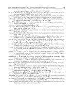
= 0). In Fig. 1 a) the quantity ξ
3
n,being
proportional to I
ν
, is plotted as a function of ξ for F = 0 and three values of E,namelyE = E
(eq)
,
E
= E
(eq)
/2, and E = 2E
(eq)
. The first case corresponds the thermal equilibrium with I
ν

= B
ν
,
while the others must have nonequilibrium populations of photon states. The results show
that the energy unbalance is mainly due to under- and overpopulation, respectively, and only
to a small extent due to a shift of the frequency maximum.
Now, consider a non-gray medium, still without scattering, but with a frequency dependent κ
ν
as follows: κ = 2κ
1
for ξ < 4, with constant κ
1
,andκ = κ
1
for ξ > 4. The important property is
that κ
ν
is larger at low frequencies and smaller at high frequencies. The resulting distribution
function, in terms of ξ
3
n, is shown in Fig. 1 b). For E = E
(eq)
, the resulting distribution
is of course still the Planck equilibrium distribution. However, for larger (smaller) energy
density the radiation density differs from the gray-matter case. In particular, the distribution
is directly influenced by the κ
ν
-spectrum. This behavior is not possible if one applies the
maximum entropy closure in the same framework of a single-band moment approximation. A
qualitative explanation of such behavior is as follows. Equilibration of the photon gas is only

possible via the interaction with matter. In frequency bands where the interaction strength,
κ
ν
,islarger(ξ < 4), the nonequilibrium distribution is pulled closer to the equilibrium
distribution than for frequencies with smaller κ
ν
. This simple argument explains qualitatively
the principal behavior associated with entropy production rate principles: the strength of the
irreversible processes determines the distance from thermal equilibrium in the presence of a
stationary constraint pushing a system out of equilibrium.
Results for the effective absorption coefficients κ
(eff)
E
and κ
(eff)
F
are shown in Fig. 2. In Fig.
2 a) it is shown that the effective absorption coefficient κ
(eff)
E
is equal to the Planck mean
(1.6κ
1
, dashed-double-dotted) in the emission limit E/E
(eq)
→ 0, and equal to the Rosseland
mean (1.26κ
1
, dashed-dotted) near equilibrium E = E
(eq)

, and eventually goes slowly to the
high frequency value κ
1
for large E. The effective absorption coefficient obtained from the
maximum entropy closure is also plotted (dotted curve), and although correct for E/E
(eq)
→0,
Fig. 1. Nonequilibrium distribution (ξ
3
n
ν
∝ I
ν
) as a function of ξ = hν/k
B
T,without
scattering, for F
= 0andE = E
(eq)
(solid), E = E
(eq)
/2 (dashed), and E = 2E
(eq)
(dotted). a)
gray matter; b) piecewise constant κ with κ
ξ<4
= 2κ
ξ>4
.
116

Heat Transfer - Mathematical Modelling, Numerical Methods and Information Technology
Radiative Heat Transfer and Effective Transport Coefficients 17
Fig. 2. a) Effective absorption coefficients for E as a function of E for F = 0, with the same
spectrum as for Fig. 1 b). Dashed-dotted: Rosseland mean; dashed-double-dotted: Planck
mean; solid: entropy production rate closure (correct at E
= E
(eq)
); dotted: entropy closure
(wrong at E
= E
(eq)
). b) Effective absorption coefficients for F as a function of v = F/E for
different E-values (dotted: E/E
(eq)
= 2; solid E/E
(eq)
= 1; dashed: E/E
(eq)
= 0.5; short-long
dashed: E/E
(eq)
= 0.05). Dashed-dotted and dashed-double dotted as in a).
it is wrong at equilibrium E
= E
(eq)
. For the present example the maximum entropy closure is
strongly overestimating the values of κ
(eff)
E
.

Figure 2 b) shows κ
(eff)
E
as a function v, for various values of E. As at constant E,increasing
v corresponds to a shift of the distribution towards higher frequencies in direction of F,a
decrease of κ
(eff)
E
must be expected, which is clearly observed in the figure.
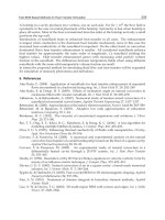
In order to investigate the effect of scattering σ
ν
= 0, we consider the example of gray
absorbing matter, i.e., constant κ
ν
≡κ
1
, having a frequency dependent scattering rate σ
ξ<4
= 0
and σ
ξ>4
= κ
1
. Scattering is only active for large frequencies. The distribution ξ
3
n
ν
of radiation
with E
= 2E

(eq)
,withfinitefluxv = 0.25 for different directions μ = cos(θ)=−1, −0.5, 0, 0.5, 1
is plotted in Fig. 3 a). Since the total energy of the photon gas is twice the equilibrium energy,
the curves are centered around about twice the equilibrium distribution. As one expects, the
states in forward direction (μ
= 1) have the highest population, while the states propagating
against the mean flux (μ
= −1) have lowest population. This behavior occurs, of course, also
in the absence of scattering. One observes that scattering acts to decrease the anisotropy of the
distribution,asforξ
> 4 the curves are pulled towards the state with μ ≈ 0. Hence, also the
effect of elastic scattering to the distribution function can be understood in the framework of
the entropy production, namely by the tendency to push the state towards equilibrium with a
strength related to the interaction with the LTE matter.
The effective absorption coefficient κ
(eff)
F
is shown in Fig. 3 b) for two values of v;itisobvious
that it must increase for increasing v and for increasing E. The Rosseland and Planck averages
of κ
ν
+ σ
ν
are given by 1.42κ
1
and 1.40κ
1
, while the emission limit for κ
(eff)
F

given in Eq. (47)
is 1.20κ
1
.
The VEF will be discussed separately in the following subsection, because its behavior has not
only quantitative physical, but also important qualitative mathematical consequences.
117
Radiative Heat Transfer and Effective Transport Coefficients
18 Heat Transfer
Fig. 3. a) Nonequilibrium distribution (ξ
3
n
ν
∝ I
ν
) as a function of ξ = hν/k
B
T,foramedium
with constant absorption κ
ν
≡ κ
1
and piecewise constant scattering with σ
ξ<4
= 0, and
σ
ξ>4
= κ
1
. The different curves refer to different radiation directions of μ = −1, −0.5, 0, 0.5, 1

(solid curves in ascending order) from photons counter-propagating to the mean drift F to
photons in F-direction. b) Effective absorption coefficients κ
(eff)
F
as a function of E/E
(eq)
for
v
= 0.25, 0.5 (solid curves in ascending order); dashed-dotted: Rosseland mean, dashed:
emission mean of κ
(eff)
F
.
5.4 The variable Eddington factor and critical points
A detailed discussion of general mathematical properties and conventional closures is given
by Levermore (1996). A necessary condition for a closure method is existence and uniqueness
of the solution. It is well-known that convexity of a minimization problem is a crucial
property in this context. One should note that convexity of the entropy production rate in
nonequilibrium situations is often introduced as a presumption for further considerations
rather than it is a proven property (cf. Martyushev (2006)). For the case without scattering,
σ
ν
≡0, Christen & Kassubek (2009) have shown that the entropy production rate (33) is strictly
convex. A discussion of convexity for a finite scattering rate goes beyond the purpose of this
chapter.
Besides uniqueness of the solution, the moment equations should be of hyperbolic type, in
order to come up with a physically reasonable radiation model. It is an advantage of the
entropy maximization closure that uniqueness and hyperbolicity are fulfilled and are related
to the convexity properties of the entropy (cf. Levermore (1996)). In the following, we provide
some basics needed for understanding the problem of hyperbolicity, its relation to the VEF

and the occurrence of critical points. The latter is practically relevant because it affects the
modelling of the boundary conditions, particularly in the context of numerical simulations.
More details are provided by K¨orner & Janka (1992), Smit et al. (1997), and Pons et al. (2000).
A list of the properties that a reasonable VEF must have (cf. Pomraning (1982)) is: χ
(v =
0)=1/3, χ(v = 1)=1, monotonously increasing χ(v ), and the Schwarz inequality v
2
≤ χ(v).
The latter follows from the fact that χ and v can be understood as averages of μ
2
and
μ, respectively, with (positive) probability density I
ν
(μ)/E . Hyperbolicity adds a further
requirement to the list. Equations (13) and (14) form a set of quasilinear first order differential
equations. For simplicity, we consider a one dimensional position space
5
with coordinate x
with 0
≤ x ≤ L,andvariablesE ≥ 0andF. In this case we redefine F, such that it can have
5
Momentum space remains three dimensional.
118
Heat Transfer - Mathematical Modelling, Numerical Methods and Information Technology
Radiative Heat Transfer and Effective Transport Coefficients 19
either sign, −E ≤ F ≤ E. We assume flux in positive direction, F ≥ 0, and write the moment
equations in the form
1
c
∂

t

E
F

+

01
∂
E
(χE) E∂
F
χ

∂
x

E
F

=

P
E
P
F

. (50)
For spatially constant E and F,smalldisturbancesofδE and δF must propagate with
well-defined speed, implying real characteristic velocities. Those are given by the eigenvalues

of the matrix that appears in the second term on the left hand side of Eq. (50) and which we
denote by M:
w
±
=
Tr M
2
±

(Tr M)
2
4
−det( M) , (51)
where ”Tr” and ”det” denote trace and determinant. Note that the w
±
are normalized to
c,i.e.
−1 ≤ w
−
≤ w
+
≤ 1 must hold. Hyperbolicity refers to real eigenvalues w
±
and
to the existence of two independent eigenvectors. The condition for hyperbolicity reads
(∂
F
(χE))
2
+ 4∂

E
(χE) > 0.
Provided hyperbolicity is guaranteed, the sign of the velocities is an issue relevant for the
boundary conditions. Indeed, the boundary condition, say at x
= L, can only have an effect
on the state in the domain if at least one of the characteristic velocities is negative. It is clear
that a disturbance near equilibrium (v
= 0) propagates in ±x direction since w
+
= −w
−
due
to mirror symmetry. Hence w
−
< 0 < w
+
for sufficiently small v. In this case boundary
conditions to both boundaries x
= 0andx = L have to be applied as in a usual boundary
value problem. However, for finite v, reflection symmetry is broken and w
+
= −w
−
.It
turns out, that for sufficiently large v,eitherw
+
or w
−
can change sign. For positive F,we
denote the value of v where w

−
becomes positive by v
c
. This is called a critical point because
det
(M)=w
+
w
−
vanishes there. Beyond the critical point, all disturbances will propagate in
positive direction, and a boundary condition at x
= L is not to be applied. This can introduce
a problem in numerical simulations with fixed predefined boundary conditions. The rough
physical meaning of the critical point is a cross-over from diffusion dominated to streaming
dominated radiation. In the latter region it might be reasonable to improve the radiation
model by involving higher order moments or partial moments, for example by decomposing
the moments in backward and forward propagating components E
±
and F
±
(cf. sect. 3.1 in
Frank (2007)).
In Fig. 4 a), different VEFs are shown. All of them exhibit the above mentioned properties,
χ
(v = 0)=1/3, monotonous increase, χ(v → 1)=1, and the Schwarz inequality v
2
≤ χ.In
particular, the VEFs obtained from entropy production rate minimization is shown for E
=
E

(eq)
for gray matter with σ
ν
≡0, as well as for the emission limit (cf. Eqs. (44) and (45)). Note
that the latter χ
(v) is a function of v only and is independent of the detailed properties of the
absorption and scattering spectra. The similarity of the differently defined VEFs, combined
with the error done anyhow by the two-moment approximation, makes it obvious that for
practical purpose the simple Kershaw VEF (j
= 2) may serve as a sufficient approximation. In
Fig. 4 b) the characteristic velocities w
±
are plotted versus v for the various VEFs discussed
above. It turns out that the VEF given by Eq. (25) has a critical point for j
> 3/2 given by v
c
=
1/
j

2(j −1), and that there is a minimum v
c
value of 0.63 at j = 3.16. The VEF by Kershaw
and maximum entropy have v
c
= 1/
√
2andv
c
= 2

√
3/5, respectively. Also the VEF associated
with the entropy production rate has generally a critical point, which depends on E. One has
to expect a typical value of v
c
≈ 2/3. For the VEF (25) with j = 1 a critical point does not
119
Radiative Heat Transfer and Effective Transport Coefficients
20 Heat Transfer
Fig. 4. a) Eddington Factors χ versus v and b) characteristic velocities w
±
for various cases.
Minimum entropy production: E
= E
(eq)
(thick solid curve) and emission limit E  E
(eq)
(thin solid curve); maximum entropy (dashed); Kershaw (dotted; j = 2 in Eq. (25)), and Auer
(dashed-dotted; j
= 1 in Eq. (25)).
appear. In the framework of numerical simulations, this advantage can outweigh in certain
situations the disadvantage of the erroneous anisotropy in the v
→ 0 limit.
6. Boundary conditions
In order to solve the moment equations, initial and boundary conditions are required. While
the definition of initial conditions are usually unproblematic, the definition of boundary
conditions is not straight-forward and deserves some remarks. In the sequel we will consider
boundaries where the characteristic velocities are such that boundary conditions are needed.
But note that the other case where boundary conditions are obsolete can also be important,
for example in stellar physics where, beyond a certain distance from a star, freely streaming

radiation completely escapes into the vacuum.
The mathematically general boundary condition for the two-moment model is of the form
aE
+ b ˆn · F = Γ , (52)
with the surface normal ˆn, and where the coefficients a, b, and the inhomogeneity Γ must be
determined from Eq. (5). There is a certain ambiguity to do this (cf. Duderstadt & Martin
(1979)) and thus a number of different boundary conditions exist in the literature (cf. Su
(2000)).
There may be simple cases where one can either apply Dirichlet boundary conditions E
(x
w
)=
E
w
to E,whereE
w
is the equilibrium value associated with the (local) wall temperature,
and/or homogeneous Neumann boundary conditions to F,
( ˆn ·∇)F = 0, at x
w
. This approach
may be appropriate, if the boundaries do not significantly influence the physics in the region
of interest, e.g., in the case where cold absorbing boundaries are far from a hot radiating object
under investigation. It can also be convenient to include in the simulation, instead of using
boundary conditions, the solid bulk material that forms the surface, and to describe it by its
κ
ν
and σ
ν
. In the next section an example of this kind will be discussed. If necessary, thermal

equilibrium boundary conditions deep inside the solid may be assumed. In this way, it is also
possible to analytically calculate the Stefan-Boltzmann radiation law for a plane sandwich
structure (hot solid body)-(vacuum gap)-(cold solid body), if an Eddington factor (25) with
j
= 1 is used and the solids are thick opaque gray bodies.
120
Heat Transfer - Mathematical Modelling, Numerical Methods and Information Technology
Radiative Heat Transfer and Effective Transport Coefficients 21
In general, however, one would like to have physically reasonable boundary conditions at
a surface characterized by Eq. (5). For engineering applications, often boundary conditions
by Marshak (1947) are used. In the following, we sketch the principle how these boundary
conditions can be derived for a simple example (cf. Bayazitoglu & Higenyi (1979)). For other
types, like Mark or modified Milne boundary conditions see, e.g. Su (2000). Let the coordinate
x
≥ 0benormaltothesurfaceatx = 0, and ask for the relation between the normal flux F, E,
and E
(eq)
w
at x = 0. The F-components tangential to the boundary are assumed to vanish, and
diffusive reflection with r
(x
w
,Ω,
˜
Ω)=r/π with r = 1 − is considered. In terms of moments,
the radiation field is given by
I
ν
=
c

4π

E
ν
P
0
(μ)+3F
ν
P
1
(μ)+
5
2
(3Π
ν,11
− E
ν
)P
2
(μ)+

, (53)
with Legendre polynomials P
0
= 1, P
1
= μ, P
2
=(3μ
2

−1)/2. The exact solution contains also
higher order Legendre polynomials, as indicated by the dots. The boundary condition (5) can
be written as
I
ν
(μ ≥ 0)=B
ν
+ 2r

0
−1
d
˜
μ |
˜
μ
| I
ν
(
˜
μ
) . (54)
By using Eq. (53), the integral can be calculated, such that the right hand side of Eq. (54)
becomes a constant with respect to μ, while the left hand side is, according to Eq. (53), a
function of μ defined for 0
≤ μ ≤ 1. In order to obtain the required relation between F and
E, one has to multiply Eq. (54) with a weight function h
(μ) and integrate over μ from 0 to 1.
The above mentioned ambiguity lies in the freedom of choice of h
(μ). Marshak (1947) selected

h
= P
1
.ProvidedP
n
for n > 3 are neglected in Eq. (53), integration leads to an inward flux
F
=

2(2 −)

E
w
−
(
3E + 15Π
11
)
8

, (55)
where Π
11
= χE. If higher order moments are to be considered, additional projections have
to be performed, in analogy to the procedure reported by Bayazitoglu & Higenyi (1979) for
the P-3 approximation.
6
For isotropic radiation with χ = 1/3, or Π
11
= E/3, the prefactor of E

becomes unity and Eq. (55) reduces to the well-known P-1-Marshak boundary condition. In
the transparent limit with χ
= 1, the prefactor becomes 9/4.
For the simple case of two parallel plane plates (
= 1) with temperatures associated with
E
w,1
and E
w,2
< E
w,1
, and separated by a vacuum gap, both moments E and F are spatially
constant and the Stefan-Boltzmann law F
=(E
(eq)
1
− E
(eq)
2
)/4 is recovered. But note that the
energy density E between the plates is not equal to the expected average of E
(eq)
1
and E
(eq)
2
,
which is an artifact of the two-moment approximation with VEF.
7. A simulation example: electric arc radiation
The two-moment approximation will now be illustrated for the example of an electric arc.

The extreme complexity of the full radiation hydrodynamics is obvious. Besides transonic
and turbulent gas dynamics, which is likely supplemented with side effects like mass ablation
and electrode erosion, a temperature range between room temperature and up to 30

000K
6
Note that neither the series (53) stops after the N’th moment (even not for the P-N approximation,
cf. Cullen (2001)), nor all higher order coefficients drop out after projection of Eq. (54) on P
n
.Ageneral
discussion, however, goes beyond this chapter and will be published elsewhere.
121
Radiative Heat Transfer and Effective Transport Coefficients
22 Heat Transfer
is covered. In this range extremely complicated absorption spectra including all kinds
of transitions occur, and the radiation is far from equilibrium although the plasma can
often be considered at LTE. Last but not least, the geometries are usually of complicated
three-dimensional nature without much symmetry, as for instance in a electric circuit breaker.
More details are given by Jones & Fang (1980), Aubrecht & Lowke (1994), Eby et al. (1998),
Godin et al. (2000), Dixon et al. (2004), and Nordborg & Iordanidis (2008).
It is sufficient for our purpose to restrict the considerations to the radiation part for a given
temperature profile, for instance of a cylindrical electric arc in a gas in front of a plate with
a slit (see Fig. 5). We may neglect scattering in the gas (σ
ν
≡ 0) and mention that an
electric arc consists of a very hot, emitting but transparent core surrounded by a cold gas,
which is opaque for some frequencies and transparent for others. First, one has to determine
the effective transport coefficients κ
(eff)
E

, κ
(eff)
F
,andχ(v), with the above introduced entropy
production minimization method. For simplicity, we assume now that this is done and these
functions are given simply by constant values listed in the caption of Fig. 5, and that χ
(v) is
well-approximated by Kershaw’s VEF. Note that due to the low density in the hot arc core, the
effective absorption coefficient there is smaller than in the surrounding cold gas. Therefore,
one expects that the radiation in the arc center will exhibit stronger nonequilibrium than in
the surrounding colder gas.
The energy density E and the velocity vectors v
= F/E obtained by a simulation with the
commercial software ANSYS
R

FLUENT
R

are shown in Fig. 5. At the outer boundaries,
homogeneous Neumann boundary conditions are used for all quantities. The wall defining
the slit is modelled as a material with either a) high absorption coefficient or b) high scattering
coefficient. The behavior of the velocity vector field clearly reflects these different boundary
properties. The E-surface plot shows the shadowing effect of the wall when the arc radiation
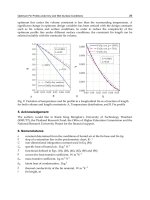
is focused through the slit. The energy densities E along the x-axis are shown in Fig. 6 a) for
the two cases. One observes the enhanced E in the region of the slit for the scattering wall.
The energy flux in physical units, i.e., cF, on the screen in front of the slit is shown in Fig. 6
b). The effect here is again what one expects: an enhanced and less focused power flux due to
the absence of absorption in the constricting wall.
8. Summary and conclusion

After a short general overview on radiative heat transfer, this chapter has focused on truncated
moment expansions of the RTE for radiation modelling. One reason for a preference of a
moment based description is the occurrence of the moments directly in the hydrodynamic
equations for the matter, and the equivalence of the type of hyperbolic partial differential
equations for radiation and matter, which allows to set complete numerical simulations on an
equal footing.
The truncation of the moment expansion requires a closure prescription, which determines the
unknown transport coefficients and provides the nonequilibrium distribution as a function
of the moments. It was the main goal of this chapter to introduce the minimum entropy
production rate closure, and to illustrate with the help of the two-moment approximation that
this closure is the one to be favored due to the following properties of the result:
– It is exact near thermodynamic equilibrium, and particularly leads to the Rosseland mean
absorption coefficients.
– It exhibits the required flux limiting behavior by yielding reasonable variable Eddington
factors.
122
Heat Transfer - Mathematical Modelling, Numerical Methods and Information Technology
Radiative Heat Transfer and Effective Transport Coefficients 23
Fig. 5. Illustrative simulations of the moment equations with FLUENT
R

for a cylindrical
electrical arc (radius 1 cm, temperature 10

000 K, κ
(eff)
E
= κ
(eff)
F

= 1/m) in a gas (ambient
temperature 300 K, κ
(eff)
E
= κ
(eff)
F
= 5/m). A solid wall (a): only absorbing with
κ
(eff)
E
= κ
(eff)
F
≡ 500/m; (b): wall with scattering coefficient, and κ
(eff)
E
= 5/m, κ
(eff)
F
≡ 500/m
with a slit in front of the arc focusing the radiation towards a wall. Surface plot for E (dark:
large, bright: small, logarithmic scale); arrows for v (not F!). Only one quadrant of the
symmetric arrangement is show.
123
Radiative Heat Transfer and Effective Transport Coefficients
24 Heat Transfer
Fig. 6. a) Energy density along the x-axis (arc center at x = 0) and b) power flux along the
screen (x
= 10cm) for the two cases Fig. 5 a) (solid) and Fig. 5 b) (dashed).

– It gives the expected results in the emission limit, and particularly leads to the Planck mean
absorption coefficient.
– It can be generalized to an arbitrary number and type of moments.
– It can be generalized to particles with arbitrary type of energy-momentum dispersion (e.g.
massive particles) and statistics (Bosons and Fermions), as long as they are described by a
linear BTE. In stellar physics, for instance, neutrons or even neutrinos can be included in
the analogous way.
The main requirement of general applicability is that the particles be independent, i.e., they
interact on the microscopic scale only with a heat bath but not among each other. On a
macroscopic scale, long-range interaction (e.g., Coulomb interaction) via a mean field may
be included for charged particles on the hydrodynamic level of the moment equations.
Independency, i.e. linearity of the underlying Boltzmann equation, has the effect that on the
level of the BTE (or RTE) nonequilibrium is always in the linear response regime. In this sense,
all transport steady-states are near equilibrium even if f
ν
strongly deviates from f
(eq)
ν
,andthe
entropy production rate optimization according to Kohler (1948) can be applied.
9. References
Abu-Romia M M and Tien C L, J. Heat Transfer 89, 321 (1967).
Anile A M, Pennisi S, and Sammartino M, J. Math. Phys. 32, 544 (1991).
Anile A, Romano V, and Russo G, SIAM J. Appl. Math. 61, 74 (2000).
Arridge S. R. et al., Med. Phys. 27, 252 (2000).
Aubrecht V, Lowke J J, J. Phys. D: Appl. Phys. 27, 2066 (1994).
Auer L H, in Methods in radiative transfer, ed. Kalkofen W, Cambridge University Press (1984).
Barichello L B and Siewert C E, Nuclear Sci. and Eng. 130,79 (1998).
Bayazitoglu Y and Higenyi J, AIAA Journal 17, 424 (1979).
Brooks E D and Fleck A, J. Comp. Phys. 67, 59 (1986).

Brooks E D et al. J. C omp. Phys. 205, 737 (2005).
Cernohorsky J and Bludman S A, The Astrophys. Jour. 443, 250 (1994).
Chandrasekhar S, Radiative Transfer, Dover Publ. Inc., N. Y. (1960).
Christen T, J. Phys. D: Appl. Phys. 40, 5719 (2007).
Christen T and Kassubek F, J. Quant. Spectrosc. Radiat. Transfer.110, 452 (2009).
124
Heat Transfer - Mathematical Modelling, Numerical Methods and Information Technology
Radiative Heat Transfer and Effective Transport Coefficients 25
Christen T Entropy 11, 1042 (2009).
Christen T, Europhys. Lett. 89, 57007 (2010).
Cullen D E and Pomraning G C, J. Quant. Spectrosc. Radiat. Transfer. 24, 97 (1980).
Cullen D E, Why ar e the P-N and the S-N methods equivalent?, UCRL-ID-145518 (2001).
Dixon C M, Yan J D, and Fang M T C, J. Phys. D : Appl. Phys 37, 3309 (2004).
Duderstadt J J and Martin W R, Transport Theory, Wiley Interscience, New York (1979).
Eby S D, Trepanier J Y, and Zhang X D, J. Phys. D: Appl. Phys. 31, 1578 (1998).
Essex C, The Astrophys. Jeut. 285, 279 (1984).
Essex C, Minimum entropy production of neutrino radiation in the steady state, Institute for
fundamental theory, UFIFT HEP-97-7 (1997).
Fort J, Physica A 243, 275 (1997).
Frank M, Dubroca B, and Klar A, J. Comput. Physics 218, 1 (2006).
Frank M, Bull. Inst. Math. Acad. Sinica 2, 409 (2007).
Fuss S P and Hamins A, J. Heat Transfer ASME 124, 26 (2002).
Godin D et al., J. Phys. D: Appl. Phys 33, 2583 (2000).
Jones G R and Fang M T C, Rep. Prog. Phys. 43, 1415 (1980).
Kabelac S, Thermodynamik der Strahlung Vieweg, Braunschweig (1994).
Kershaw D, Flux limiting nature’s own way, Lawrence Livermore Laboratory, UCRL-78378
(1976).
Kohler M, Z. Physik 124, 772 (1948).
K¨orner A and Janka H-T, Astron. Astrophys. 266, 613 (1992).
Kr¨oll W, J. Quant. Spectrosc. Radiat. Transfer. 7, 715 (1967).

Landau L D and Lifshitz E M, Statistical Physics, Elsevier, Amsterdam (2005).
Levermore C D, J. Quant. Spectrosc. Radiat. Transfer. 31, 149 (1984).
Levermore C D, J. Stat. Phys. 83, 1021 (1996).
Levermore C D and Pomraning G C, The Astrophys. Jou. Y 248, 321 (1981).
Lowke J J, J. Appl. Phys. 41, 2588 (1970).
Marshak R E, Phys. Rev. 71, 443 (1947).
Martyushev L M and Seleznev V D, Phys. Rep. 426, 1 (2006).
Minerbo G N, J. Quant. Spectrosc. Radiat. Transfer. 20, 541 (1978).
Mihalas D and Mihalas B W, Foundations of Radiation Hydrodynamics, Oxford University Press,
New York (1984).
Modest M, Radiative Heat Transfer, Elsevier Science, (San Diego, USA, 2003).
Nordborg H and Iordanidis A A, J. Phys. D: Appl. Phys. 41, 135205 (2008).
Olson G L, Auer L H, and Hall M L, J. Quant. Spectrosc. Radiat. Transfer. 64, 619 (2000).
Oxenius J, J. Quant. Spectrosc. Radiat. Transfer. 6, 65 (1966).
Patch R W, J. Quant. Spectrosc. Radiat. Transfer. 7, 611 (1967).
Planck M, Vorlesungen ¨uber die T heorie der W¨armestrahlung, Verlag J. A. Barth, Leipzig (1906).
Pons J A, Ibanez J M, and Miralles J A, Mon. Not. Astron. Soc. 317, 550 (2000).
Pomraning G C, J. Quant. Spectrosc. Radiat. Transfer. 26, 385 (1981).
Pomraning G C, Radiation Hydrodynamics Los Alamos National Laboratory, LA-UR-82-2625
(1982).
Rey C C, Numerical Methods for radiative transfer, PhD Thesis, Universitat Politecnica de
Catalunya (2006).
Ripoll J-F, Dubroca B, and Duffa G, Combustion Theory and Modelling 5, 261 (2001).
Ripoll J-F , J. Quant. Spectrosc. Radiat. Transfer. 83, 493 (2004).
Ripoll J-F and Wray A A, J. Comp. Phys. 227, 2212 (2008).
125
Radiative Heat Transfer and Effective Transport Coefficients
26 Heat Transfer
Sampson D H, J. Quant. Spectrosc. Radiat. Transfer. 5, 211 (1965).
Santillan M, Ares de Parga G, and Angulo-Brown F, Eur. J. Phys. 19, 361 (1998).

Seeger M, et al. J. Phys. D: Appl. Phys 39, 2180 (2006).
Siegel R and Howell J R, Thermal radiation heat transfer, Washington, Philadelphia, London;
Hemisphere Publ. Corp. (1992).
Simmons K H and Mihalas D, J. Quant. Spectrosc. Radiat. Transfer. 66, 263 (2000).
Smit J M, Cernohorsky J, and Dullemond C P Astron. A strophys. 325, 203 (1997).
Struchtrup H, Ph. D. Thesis TU Berlin (1996).
Struchtrup H, in Rational extended thermodynamics ed. M ¨uller I. and Ruggeri T., Springer, New.
York, Second Edition, p. 308 (1998).
Su B, J. Quant. Spectrosc. Radiat. Transfer. 64, 409 (2000).
Tien C L, Radiation properties of gases,inAdvances in heat transfer, Vol.5, Academic Press, New
York (1968).
Turpault R, J. Quant. Spectrosc. Radiat. Transfer. 94, 357 (2005).
W¨urfelPandRuppelW,J. Phys. C: Solid State Phys. 18, 2987 (1985).
Yang W-J, Taniguchi H, and Kudo K, Radiative Heat Transfer by the Monte Carlo Method,
Academic Press, San Diego (1995).
Ziman J M, Can. J. Phys. 34, 1256 (1956).
Zhang J F, Fang M T C, and Newland D B, J. Phys. D: Appl. Phys 20, 368 (1987).
126
Heat Transfer - Mathematical Modelling, Numerical Methods and Information Technology
Part 2
Numerical Methods and Calculations

0
Finite Volume Method Analysis of Heat Transfer in
Multi-Block Grid During Solidification
Eliseu Monteiro
1
, Regina Almeida
2
and Abel Rouboa

3
1
CITAB/UTAD - Engineering Department of
University of Tr´as-os-Montes e Alto Douro, Vila Real
2
CIDMA/UA - Mathematical Department of
University of Tr´as-os-Montes e Alto Douro, Vila Real
3
CITAB/UTAD - Department of Mechanical Engineering and
Applied Mechanics of University of Pennsylvania, Philadelphia, PA
1,2
Portugal
3
USA
1. Introduction
Solidification of an alloy has many industrial applications, such as foundry technology, crystal
growth, coating and purification of materials, welding process, etc. Unlike the classical
Stefan problem for pure metals, alloy solidification involves complex heat and mass transport
phenomena. For most metal alloys, there could be three regions, namely, solid region, mushy
zone (dendrite arms and interdendritic liquid) and liquid region in solidification process.
Solidification of binary mixtures does not exhibit a distinct front separating solid and liquid
phases. Instead, the solid is formed as a permeable, fluid saturated, crystal-line-like matrix.
The structure and extent of this mushy region, depends on numerous factors, such as the
specific boundary and initial conditions. During solidification, latent energy is released at
the interfaces which separate the phases within the mushy region. The distribution of this
energy therefore depends on the specific structure of the multiphase region. Latent energy
released during solidification is transferred by conduction in the solid phase, as well as by
the combined effects of conduction and convection in the liquid phase. To investigate the
heat and mass transfer during the solidification process of an alloy, a few models have been
proposed. They can be roughly classified into the continuum model and the volume-averaged

model. Based on principles of classical mixture theory, Bennon & Incropera (1987) developed
a continuum model for momentum, heat and species transport in the solidification process
of a binary alloy. Voller et al. (1989) and Rappaz & Voller (1990) modified the continuum
model by considering the solute distribution on microstructure, the so-called Scheil approach.
Beckermann & Viskanta (1988) reported an experimental study on dendritic solidification
of an ammonium chloride-water solution. A numerical simulation for the same physical
configuration was also performed using a volumetric averaging technique. Subsequently, the
volumetric averaging technique was systematically derived by Ganesan & Poirier (1990) and
Ni & Beckermann (1991). Detailed discussions on microstructure formation and mathematical
modelling of transport phenomenon during solidification of binary systems can be found in
5
2 Heat Transfer
the reviews of Rappaz (1989) and Viskanta (1990).
In the last few decades intensive studies have been made to model various problems,
for example: to solve radiative transfer problem in triangular meshes, Feldheim & Lybaert
(2004) used discrete transfer method (DTM can be see in the work of Lockwood & Shah
(1981)), Galerkin finite element method was used by Wiwatanapataphee et al. (2004) and
Tryggvason et al. (2005) to study the turbulent fluid flow and heat transfer problems in a
domain with moving phase-change boundary and Dimova et al. (1998) also used Galerkin
finite element method to solve nonlinear phenomena. Finite volume method for the
calculation of solute transport in directional solidification has been studied and validated
by Lan & Chen (1996). Finite element method to model the filling and solidification inside
a permanent mold is performed by Shepel & Paolucci (2002). Three dimensional parallel
simulation tool using a unstructured finite volume method with Jacobian-free Newton-Krylov
solver, has been done by Knoll et al. (2001) for solidifying flow applications. Also arbitrary
Lagrangian-Euler (ALE) formulation was develop by Bellet & Fachinotti (2004) to simulate
casting processes, among others. One of the major challenges of heat transfer modelling of
molten metal has been the phase change. To model such a phase change requires the strict
imposition of boundary conditions. Normally, this could be achieved with a finite-element
that is distorted to fit the interface. Since the solid-liquid phase boundaries are moving

the use of level set methods are a recent trend (Sethian (1996)). However, both of these
techniques are computationally expensive. The classical fixed mesh is computational less
expensive but could not been able to maintain the correct boundary conditions. In this
regard, Monteiro (1996) studied the application of the finite difference method to permanent
mold casting using generalized curvilinear coordinates. A multi-block grid was applied to
a complex geometry and the following boundary conditions: continuity condition to virtual
interfaces and convective heat transfer to metal-mold and mold-environment interfaces. The
reproduction of this simulation procedure using the finite volume method was made by
Monteiro (2003). The agreement with experimental data was also good. Further developments
of this work were made by Monteiro & Rouboa (2005) where more reliable initial conditions
and two different kinds of boundary conditions were applied with an increase in agreement
with the experimental data. In the present work we compare the finite difference and finite
volume methods in terms of space discretization, boundary conditions definition, and results
using a multi-block grid in combination with curvilinear coordinates. The multi-block grid
technique allows artificially reducing the complexity of the geometry by breaking down
the real domain into a number of subdomains with simpler geometry. However, this
technique requires adapted solvers to a nine nodes computational cell instead of the five
nodes computational cell used with cartesian coordinates for two dimensional cases. These
developments are presented for the simple iterative methods Jacobi and Gauss-Seidel and also
for the incomplete factorization method strongly implicit procedure.
2. Heat transfer and governing equations
Solidification modelling can be divided into three separate models, where each model
is identified by the solution to a separate set of equations: heat transfer modelling which
solves the energy equation; fluid-flow modelling which solves the continuity and momentum
equations; and free-surface modelling which solves the surface boundary conditions. For a
complete description of a casting solidification scenario, all these equations should be solved
simultaneously, but under special circumstances they could be decoupled and modelled
independently. This is the case for heat-transfer modelling, which has been widely used, and
130
Heat Transfer - Mathematical Modelling, Numerical Methods and Information Technology

Finite Volume Method Analysis of Heat Transfer in
Multi-Block Grid During Solidification
3
its application has significantly improved casting quality (Swaminathan & Voller (1997)).
2.1 Mathematical model
The governing system equations is composed by the heat conservative equation, the boundary
condition equations and the initial equation. In this section, differential equations of the
heat conservative and adapted boundary conditions for the solidification phenomena will be
presented.
2.1.1 Energy conservation equation
The energy conservation equation states that the rate of gain in energy per unit volume equals
the energy gained by any source term, minus the energy lost by conduction, minus the rate of
work done on the fluid by pressure and the viscous forces, per unit time. Assuming that:
the fluid is isotropic and obeys Fourier’s Law; the fluid is incompressible and obeys the
continuity equation; the fluid conductivity is constant; viscous heating is negligible, and since
the heat capacity of a liquid at constant volume is approximately equal to the heat capacity at
constant pressure, then, the internal energy equation is reduced to the familiar heat equation,
here shown in curvilinear coordinates (Monteiro et al. (2006), Monteiro & Rouboa (2005)). The
governing differential equation for the solidification problem may be written in the following
conservative form
∂
(
ρC
P
φ
)
∂t
= ∇·
(
k∇φ

)
+
˙
q,(1)
where
∂
(
ρC
P
φ
)
∂t
represents the transient contribution to the conservative energy equation (φ
temperature);
∇·
(
k∇φ
)
is the diffusive contribution to the energy equation and
˙
q represents
the energy released during the phase change. The physical properties of the metal: the
metal density ρ (kg/m
3
), the heat capacity of constant pressure C
P
(J/kg
o
C) and the thermal
conductivity k (W/m

o
C) are considered to be constants analogously as done by Knoll et al.
(2001), Monteiro (1996) and Shamsundar & Sparrow (1975).
The term
˙
q can be expressed as a function of effective solid (Monteiro (1996)), (s solidus or
solidified metal) material fraction f
s
, metal density ρ, and enthalpy variation during the
phase change Δh
f
called latent heat (Monteiro & Rouboa (2005), Monteiro et al. (2006)), by
the following expression
˙
q
=
∂

ρΔh
f
f
s

∂t
.(2)
One can also decompose f
s
in the following way
∂ f
s

∂t
=
∂ f
s
∂φ
∂φ
∂t
.(3)
Assuming that Δh
f
is independent of temperature and the material is isotropic, one substitutes
equations (2) and (3) in equation (1) and obtain
∂φ
∂t

1
−
Δh
f
C
P
∂ f
s
∂φ

= a


2
φ


,(4)
where a is the thermal diffusivity which is equal to a
=
k
ρC
p
(m
2
/s).
The solid fraction can be determined, at each temperature, by the lever rule. When dealing
131
Finite Volume Method Analysis of Heat Transfer in Multi-Block Grid During Solidification
4 Heat Transfer
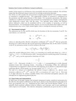
Fig. 1. Typical cooling diagram of alloys
with small temperature difference, a linear relationship between f
s
(φ) and φ, is an acceptable
approximation as shown in the Fig. 1. Thus,
∂ f
s
∂φ
can be considered as constant. The constant
φ
s
is the solidus temperature, φ
l
is the liquidus temperature and during the mushy phase
the material fraction f
s

is given by f
s
=
C
l
−C
C
l
−C
s
,whereC is the concentration, C
l
and C
s
are,
respectively, the liquidus and solidus concentrations. This assumption allows the linearization
of the source term of the energy equation.
One also uses the curvilinear coordinates which transforms the domain into rectangular and
time independent. The calculation is given by a uniform mesh of squares in a two dimension,
by the following transformation: x
i
= x
i
(ξ
1
,ξ
2
),fori = 1, 2, characterized by the Jacobian J
J
= det


∂x
i
∂ξ
j

i,j
.(5)
Therefore,
∂φ
∂x
i
=
∂φ
∂ξ
j
∂ξ
j
∂x
i
=
∂φ
∂ξ
j
β
ij
J
,(6)
where β
ij

=(−1)
i+j
det(J
ij
) represents the cofactor in the Jacobian J,andJ
ij
is the Jacobian
matrix taking out the line i and column j. Substituting the equation (6) in equation (4) one
obtains
J
∂φ
∂t

1
−
Δh
f
C
P
∂ f
s
∂φ

= a
∂
∂ξ
j

1
J


∂φ
∂ξ
m
B
mj

,(7)
where the coefficient B
mj
are defined by
B
mj
= β
kj
β
km
= β
1j
β
1m
+ β
2j
β
2m
.(8)
132
Heat Transfer - Mathematical Modelling, Numerical Methods and Information Technology
Finite Volume Method Analysis of Heat Transfer in
Multi-Block Grid During Solidification

5
The coefficient B
mj
becomes zero when the grid is orthogonal, therefore the use of these
coefficients in the equation (7).
The second term of equation (7) can be expressed by
J
∂φ
∂t

1
−
Δh
f
C
P
∂ f
s
∂φ

= C
1
∂φ
∂ξ
1
+ C
2
∂φ
∂ξ
2

+ C
11
∂
2
φ
∂ξ
2
1
+ C
12
∂
2
φ
∂ξ
1
∂ξ
2
+ C
22
∂
2
φ
∂ξ
2
2
,(9)
where
C
1
=

∂J
−1
∂ξ
1
B
11
+
∂J
−1
∂ξ
2
B
12
+ J
−1

∂B
11
∂ξ
1
+
∂B
12
∂ξ
2

,
C
2
=

∂J
−1
∂ξ
1
B
21
+
∂J
−1
∂ξ
2
B
22
+ J
−1

∂B
21
∂ξ
1
+
∂B
22
∂ξ
2

,
C
11
= J

−1
B
11
, C
12
= J
−1

B
21
+ B
12

, C
22
= J
−1
B
22
.
2.1.2 Boundary conditions
In the present study heat transfer between cast part (p), mold (m) and environment (e) is
investigated. The parameters of thermal behavior of the part/mold boundary govern the heat
transfer, determining solidification progression. The heat flow through an interface will be
the result of the combination of several modes of heat transfer. Furthermore, the value of
the heat transfer coefficient varies with several factors. It is generally accepted that the heat
transfer resistance at the interface originates from the imperfect contact or even separation of
the cast part metal and the mold. It means a gap is formed between the casting and the mold
during the casting (Wang & Matthys (2002), Lau et al. (1998)). Different possibilities must be
considered for heat transfer conditions on the boundary:

i) Continuity condition

∂φ
∂n

m
1
=

∂φ
∂n

m
2
, φ
m
1
= φ
m
2
(10)
is considered for the boundaries within continuous contact materials m
1
and m
2
(Monteiro
(1996)). This means that the heat flux is fully transferred from the material m
1
to material
m

2
without heat lost. These two materials are represented as blocks in the next sections.
ii) For the interface between different kind of materials, convective heat transfer is considered
k
m

∂φ
∂n

m
= h
∗

φ
p
−φ
m

, (11)
where φ
m
is the mold temperature, φ
p
is the cast part temperature, h
∗
is the convective heat
transfer coefficient and k
m
in the thermal conductivity of the mold.
iii) For the exterior boundary in contact with the environment we have convection and

radiation. From the work of Shi & Guo (2004) one has a mixed convection-radiation
boundary condition given by
k
m

∂φ
∂n

m
= h
cr
(
φ
m
−φ
e
)
, (12)
133
Finite Volume Method Analysis of Heat Transfer in Multi-Block Grid During Solidification