Heat Transfer Theoretical Analysis Experimental Investigations and Industrial Systems Part 6 pot

Applications of Nonstandard Finite Difference Methods to Nonlinear Heat Transfer Problems

189
The simple linear diffusion problem in one space variable
x and time
τ
, for
( , ) (0, ) (0, ),xl
τ
∈×∞ is (J. D. Smith, 1985)

2
2

TT
X
κ
τ
∂∂
=
∂
∂
(2.2)
The non-dimensionalizing process is illustrated below with the parabolic heat conduction
equation (2.2).
Work Example 1: (Involves only heat conduction)

The solution of Eq. (2.2) gives the temperature
T at a distance X from one end of a thin
uniform wire after a time .
τ
This assumes the rod is ideally heat insulated along its length
and heat transfers at its ends. Let
l represent the length of the wire and T
0
some particular
non negative constant temperature such as the maximum or minimum temperature at zero
time.
Using the following dimensionless variables

2
0
, = = ,,uTT xX tll
κτ
=
/
// (2.3)
equation (2.2) with the general boundary condition and specific initial temperature
distribution, can be rewritten in the following dimensionless form

12

, ( , ) (0,1) (0, );
(0, ) , (1, ) , 0;

(,0) 2, [0,1/2];
(,0) 2(1 ), [0,1/2];
txx
uu xt
utU utU t
ux x x
ux x x
=∈×∞
⎧

⎪
==>
⎪
⎨
=∈
⎪
⎪
=− ∈
⎩
(2.4)
where
1

U and
2
U are the dimensionless forms of
1
T and
2
T , respectively.
In other word we are seeking a numerical solution of
2
2
uu
t

x
∂
∂
=
∂
∂
which satisfies
Case I:
i. 0 0 0 0u at x and u at x l for all t== == >
.
ii. 0 : 2 0 1/2 2(1 ) 1 /2 1,for t u x for x and u x for x= = ≤≤ = − ≤≤
Case II:

iii. 0 0 0 0u at x and u at x l for all t== == >.
iv. 0 : sin 0 1.for t u x for x
π
== ≤≤
where (i), (iii) and (ii), (iv) are called the boundary condition and the initial condition
respectively.
2.2 Convection
Convection is the transfer of heat by the actual movement of the warmed matter. It is a heat
transfer through moving fluid, where the fluid carries the heat from the source to
destination. For example heat leaves the coffee cup as the currents of steam and air rise.
Convection is the transfer of heat energy in a gas or liquid by movement of currents. It can
Heat Transfer - Mathematical Modelling, Numerical Methods and Information Technology

190
also happen in some solids, like sand. More clearly, convection is effective in gas and fluids
but it can happen in solids too. The heat current moves with the gas and fluid in the most of
the food cooking. Convection is responsible for making macaroni rise and fall in a pot of
heated water. The warmer portions of the water are less dense and therefore, they rise.
Meanwhile, the cooler portions of the water fall because they are denser.
While heat convection and conduction require a medium to transfer energy, heat radiation
does not. The energy travels through nothingness (vacuum) in the heat radiation.
2.3 Radiation
Electromagnetic waves that directly transport energy through space is called radiation. Heat
radiation transmits by electromagnetic waves that travel best in a vacuum. It is a heat

transfer due to emission and absorption of electromagnetic waves. It usually happens within
the infrared/visible/ultraviolet portion of the spectrum. Some examples are: heating
elements on top of toaster, incandescent filament heats glass bulb and sun heats earth.
Sunlight is a form of radiation that is radiated through space to our planet without the aid of
fluids or solids. The sun transfers heat through 93 million miles of space. There are no solids
like a huge spoon touching the sun and our planet. Thus conduction is not responsible for
bringing heat to Earth. Since there are no fluids like air and water in space, convection is not
responsible for transferring the heat. Therefore, radiation brings heat to our planet.
Heat excites the black surface of the vanes more than it heats the white surface. Black is a
good absorber and a good radiator. Think of black as a large doorway that allows heat to
pass through easily. In contrast, white is a poor absorber and a poor radiator of energy.
White is like a small doorway and will not allow heat to pass easily.

Note that heat transfer problems involve temperature distribution not just temperature.
Heat transfer rates are determined knowing the temperature distribution. While Fourier’s
law of conduction provides the rate of heat transfer related to heat distribution, temperature
distribution in a medium governs with the principle of conservation of energy.
2.3.1 Stefan-Boltzmann radiation law
If a solid with an absolute surface temperature of T is surrounded by a gas at temperature
T
∞
, then heat transfer between the surface of the solid and the surrounding medium will
take place primarily by means of thermal radiation if
TT
∞

− is sufficiently large (P. M.
Jordan, 2003). Mathematically, the rate of heat transfer across the solid-gas interface is given
by the Stefan-Boltzmann radiation law

44
() (),
s
Tn ATT
κσε
∞
∂∂=− −/ (2.5)
where ( )

s
Tn∂∂/ the thermal gradient at the surface of the solid is evaluated in the direction
of the outward-pointing normal to the surface,
A is radiating area and 0
κ
> is the thermal
conductivity of the solid (assumed constant). The constants
ε
∈
[0,1], ( 1
ε
= for ideal

radiator while for a prefect insulator 0
ε
=
) and
24
W
8
m5.67 10 ( K )
σ
−
≈× / are, respectively,
the emissivity of the surface and the Stefan-Boltzmann constant (P. M. Jordan, 2003).

Mathematically, the rate of heat transfer across the solid-gas interface is given by the
Newton’s law of cooling (H. S. Carslaw & J. C. Jaeger, 1959; R. Siegel & J. H. Howell, 1972)
()(),
s
Tn hATT
κ
∞
∂∂=− −/ (2.6)
Applications of Nonstandard Finite Difference Methods to Nonlinear Heat Transfer Problems

191
where h is the convection heat transfer coefficient and A is cooloing area.

The applications of thermal radiation with/without conduction can be observed in a good
number of science and engineering fields including aerospace engineering/design, power
generation, glass manufacturing and astrophysics (R. Siegel & J. H. Howell, 1972; L. C.
Burmeister, 1993; M. N. Ozisik, 1989; J. C. Jaeger, 1950; E. Battaner, 1996).
In the following Work Examples we consider two problems that involve various heat
transfer properties in a thin finite rod (A. Mohammadi & A. Malek, 2009).
3. Nonlinear heat transfer in a finite thin wire
3.1 Heat transfer involving both conduction and radiation
In the following example we consider a problem that involves both conduction and
radiation and no convection.
Consider a very thin, homogeneous, thermally conducting solid rod of constant cross-
sectional area

,A perimeter ,
p
length l and constant thermal diffusivity 0
κ
> that
occupies the open interval (
0,l ) along the X - axis of a Cartesian coordinate system. That T
the temperature distribution of the rod, is
(,)TX
τ
, and
0

sin( )TXl
π
/
is initial temperature
of the rod, and let the ends at
0,Xl
=
be maintained at the constant temperatures
1
T and
2
T respectively and T

∞
the surrounding temperature. The parabolic one-dimensional
unsteady heat conduction model in a thin finite rod that is radiating heat across its lateral
surface into a medium of constant temperature is the mathematical model of this physical
system consists of the following initial boundary value problem (P. M. Jordan, 2003;
W. Dai & S. Su, 2004)

44
0
12
0
(), (,)(0,)(0,);

(0, ) , ( , ) , 0;
(,0) sin( ), (0,);
XX
TT TT X l
TTTlT
TX T X l X l
τ
κβ τ
τττ
π
∞
⎧

=− − ∈×∞
⎪
==>
⎨
⎪
=∈
⎩
/
(3.1)
where time
τ
is a non-negative variable,

0
p
KA
βκσε
=
/
in wich K is relative thermal
diffusivity constant and A stands for radiation area, and based on physical considerations,
T is assumed to be nonnegative.
Work Example 2: (Involves heat conduction and heat radiation)
Using the following dimensionless variables

2
0
32
00
, = = ,
, ,
,uTT xX t
Tl p KA u T T
ll
κτ
βσε
∞∞

=
==
/
//
//
(3.2)
where
0
0T > is taken as constant, problem (3.1) can be rewritten in dimensionless form as
follows (P. M. Jordan, 2003; W. Dai & S. Su, 2004):

44

12
(), (,)(0,1)(0,);
(0,) , (1,) , 0;
( ,0) sin , (0,1);
txx
uu uu xt
utU utU t
ux x x
β
π
∞
⎧

=− − ∈ ×∞
⎪
==>
⎨
⎪
=∈
⎩
(3.3)
where
1
U and
2

U are the dimensionless forms of
1
T and
2
T , respectively.
Heat Transfer - Mathematical Modelling, Numerical Methods and Information Technology

192
3.2 Heat transfer in a finite thin rod with additional convection term
Problem (3.1) with additional convection term becomes:

44

00
12
0
( ) ( ), ( , ) (0, ) (0, );
(0, ) , ( , )= , 0;
(,0) sin( ), (0,);
XX
TT TT TTX l
TTTlT
TX T X l X l
τ
κβ α τ

τττ
π
∞∞
⎧
=− −−− ∈×∞
⎪
=>
⎨
⎪
=∈
⎩
/

(3.4)
where
τ
the temporal is a non-negative variable,
0
,
p
KA
βκσε
= /
0
,h

p
KA/
ακ
= and
based on physical considerations,
T
is assumed to be nonnegative.
Work Example 3: (Involve conduction, radiation and convection terms)
Using the following dimensionless variables,

232
00

2
0
, = = , ,
, ,
,uTT xX t Tl
p
KA
lhp KA u T T
ll
/
κτ β σε
α

∞∞
==
==
/// /
/
(3.5)
where T
0
> 0 is taken as constant, problem (3.4) can be rewritten in dimensionless form as
follows:

44

12
()(), (,)(0,1)(0,);
(0, ) , (1, ) , 0;
(,0) sin , (0,1);
txx
uu uu uu xt
utU utU t
ux x x
βα
π
∞∞
⎧

=− −− − ∈ ×∞
⎪
==>
⎨
⎪
=∈
⎩
(3.6)
where U
1
and U
2

are the dimensionless forms of T
1
and T
2
, respectively.
In the following we propose six nonstandard explicit and implicit schemes for problem (3.6).
Novel heat theory (Microscale)
Tzou (D. Y. Tzou, 1997) has shown that if the scale in one direction is at the microscale (of
order 0.1 micrometer) then the heat flux and temperature gradient occur in this direction at
different times. Thus the heat conduction equations used to describe the microstructure
thermodynamic behavior are:
.

p
T
qQ c
ρ
τ
∂
−∇ + =
∂
and ( , ) ( , ) ,
QT
Qr Tr
τ

τκττ
+
=− ∇ +
where ,
p
c
ρ
and Q are density, a specific heat and a heat source,
Q
τ
and
T

τ
are the time lags
of the heat flux and temperature gradient which are positive constants.
Now we can introduce (A. Malek & S. H. Momeni-Masuleh, 2008) the novel heat equation as:

2333
2
2222
()( )
()
p
qq T

q
c
TT TT T
T
xy z
Q
Q
ρ
ττ τ
κτ
ττττ
τ

τ
κ
∂∂ ∂ ∂ ∂
+
=∇ + + + +
∂
∂∂∂∂∂∂∂
∂
+
∂
(3.7)
Malek and Momeni-Masuleh in years 2007 and 2008 used various hybrid spectral-FD methods

to solve Eq. (3.7) efficiently. H. Heidari and A. Malek, studied null boundary controllability for
hyperdiffusion equation in year 2009. Heidari, H. Zwart, and Malek, in year 2010 discussed
Applications of Nonstandard Finite Difference Methods to Nonlinear Heat Transfer Problems

193
controllability and stability of the 3D novel heat conduction equation in a submicroscale thin
film. In this Chapter we consider the heat theory for macroscale objects. Thus we do not
consider the numerical solution for Eq. (3.7) that is out of the scope of this chapter.
4. Finite difference methods
4.1 Standard finite difference methods
In this section, we shall first consider two well known standard finite difference methods and
their general discretization forms. Second, we shall introduce semi-discretization and fully

discretization formulas. Third we will consider consistency, convergence and stability of the
schemes. We will consider the nonlinear heat transfer problems in the next section during the
study of nonstandard FD methods. This, as we shall see, leads to discovering some efficient
algorithms that exists for corresponding class of nonlinear heat transfer problems.
Among the class of standard finite difference schemes, two important and richly studied
subclasses are explicit and implicit approaches.
Notation
It is useful to introduce the following difference notation for the first derivative of a function
u
in the
x
direction at discrete point j throughout this Chapter.

1
1
1/2 1/2
()
()
()
jj
j
jj
j
jj
j

uu
u
Forward Finite Difference
xx
uu
u
Backward Finite Difference
xx
uu
u
Central Finite Difference
xx

+
−
+−
−
∂
=
∂Δ
−
∂
=
∂Δ
−

∂
=
∂
Δ

The equation
2
2
uu
t
x
∂∂

=
∂
∂
may be approximated at the point (,)ixjt
Δ
Δ by the difference
equation:
,1 , 1,1 ,1 1,1 1, , 1,
2
(2 )(1)(2 )
,
()

i
j
i
j
i
j
i
j
i
j
i
j

i
j
i
j
uu u uu u uu
t
x
θθ
++++−++−
−−++−−+
=
Δ

Δ

for
01,
θ
≤≤
where
,
(,)
ij
uuix
j

t
=
ΔΔ
for 1, and 1, , in the iNj J xt
=
=− plane. Note that
0
θ
= gives the explicit scheme and 1 /2
θ
=
represents the Crank-Nicolson method that is

one of the famous implicit FD schemes.
4.1.1 Explicit standard FD scheme ( 0
θ
=
)
We calculate an explicit standard finite difference solution of the problem given in Work
Example 1 for both Cases I and II, where the closed analytical form solutions are
22
22
0
811
(sin )(sin )

2
nt
n
Unnxe
n
π
ππ
π
∞
−
=
=

∑
and
2
sin
t
Ue x
π
π
−
= respectively.
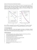
Figs. 1, 2, 3 and 4 display the power of both numerical schemes (Explicit and Crank-
Nicolson) for the calculation of the solution for problems given in Work Example 1.

Heat Transfer - Mathematical Modelling, Numerical Methods and Information Technology

194
0 0.1 0.2 0.3 0.4 0.5 0.6 0.7 0.8 0.9 1
0
0.1
0.2
0.3
0.4
0.5
0.6
0.7

0.8
0.9
1
x
U
h=0.1, k=0.001, r=0.1


Finite-Difference Explicit Method
Analytical

Fig. 1. Standard explicit FD solution of Work Example 1, Case I.

Fig. 2. Standard explicit FD solution of Work Example 1, Case II.
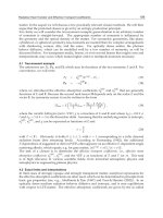
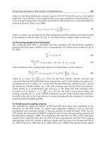
4.1.2 Crank-Nicolson standard FD scheme ( 1/2
θ
=
)
We calculate a Crank-Nicolson implicit solution of the problem given in Work Example 1 for
Case I and Case II.
Applications of Nonstandard Finite Difference Methods to Nonlinear Heat Transfer Problems

195

Fig. 3. Crank-Nicolson implicit FD solution for Work Example 1, Case I.


Fig. 4. Crank-Nicolson implicit FD solution of Work Example 1, Case II.
Up to this point most of our discussion has dealt with standard finite difference methods for
solving differential equations. We have considered linear equations for which there is a
well-designed and extensive theory. Some simple diffusion problems without nonlinear
Heat Transfer - Mathematical Modelling, Numerical Methods and Information Technology

196
terms were considered in Section 4.1. Now we must face the fact that it is usually very

difficult, if not impossible, to find a solution of a given differential equation in a reasonably
suitable and unambiguous form, especially if it involves the nonlinear terms. Therefore, it is
important to consider what qualitative information can be obtained about the solutions of
differential equation, particularly nonlinear terms, without actually solving the equations.
4.2 Nonstandard finite difference methods
Nonstandard finite difference methods for the numerical integration of nonlinear
differential equations have been constructed for a wide range of nonlinear dynamical
systems (P. M. Jordan, 2003; W. Dai & S. Su, 2004; H. S. Carslaw & J. C. Jaeger, 1959; R.
Siegel & J. H. Howell, 1972; L. C. Burmeister, 1993). The basic rules and regulations to
construct such schemes (R. E. Mickens, 1994), are:
Regulation 1. To do not face numerical instabilities, the orders of the discrete derivatives
should be equal to the orders of the corresponding derivatives appearing in the differential

equations.
Regulation 2. Discrete representations for derivatives must have nontrivial denominator
functions.
Regulation 3. Nonlinear terms should be replaced by nonlocal discrete representations.
Regulation 4. Any particular properties that hold for the differential equation should also
hold for the nonstandard finite difference scheme, otherwise numerical instability will
happen.
Positivity, boundedness, existence of special solutions and monotonicity are some properties
of particular importance in many engineering problems that usually model with differential
equations. Regulation number four restricts one to force the nonstandard scheme satisfying
properties of differential equation.
In the last two decays, several nonstandard finite difference schemes have been developed

for solving nonlinear partial differential equations by Mickens and his co-authors.
Particularly, Jordan and Dai considered a problem of one-dimensional unsteady heat
conduction in a thin finite rod that is radiating heat across its lateral surface into a medium
of constant temperature. The most fundamental modes of heat transfer are conduction and
thermal radiation. In the former, physical contact is required for heat flow to occur and the
heat flux is given by Fourier’s heat law. In the latter, a body may lose or gain heat without
the need of a transport medium, the transfer of heat taking place by means of
electromagnetic waves or photons.
In the reminder of this Chapter, we consider twelve nonstandard implicit and explicit
difference schemes for nonlinear heat transfer problems involving conductions and
radiation with or without convection term. Specifically, we employ the highly successful
nonstandard finite difference methods (A. Mohammadi, & A. Malek, 2009) to solve the

nonlinear initial-boundary value problems in Work Examples 2 and 3 (see Section 3). We
show that the third implicit schemes are unconditionally stable for large value of the
equation parameters with or without convection term. It is observed that the rod reaches
steady state sooner when it is exposed both to the radiation heat and convection.
4.1 Explicit nonstandard FD schemes
4.1.1 Nonstandard FD explicit schemes for Work Example 2
In Ref. (P. M. Jordan, 2003; W. Dai & S. Su, 2004), three nonstandard explicit finite difference
schemes for Eq. (3.3) are developed as follows:
Applications of Nonstandard Finite Difference Methods to Nonlinear Heat Transfer Problems

197

4
,1,1,
,1
3
,
(1 2 ) ( ) ( )
,
1()()
ij i j i j
ij
ij
urruu tu

u
tu
β
β
−
+∞
+
−+ + +Δ
=
+Δ
(4.1)

4
,1,1,
,1
33
1, 1,
(1 2 ) ( ) ( )
,
1()( )2
ij i j i j
ij
ij ij
urruu tu

u
tu u
β
β
−
+∞
+
−+
−+ + +Δ
=
+Δ +
(4.2)

and

22
,1,1,,,
,1
22
,,
(12)( )()()()
,
1 ( )( )( )
ij i j i j ij ij
ij

ij ij
u rru u tuuuuu
u
tu u u u
β
β
−
+∞∞∞
+
∞∞
−+ + +Δ + +
=

+Δ + +
(4.3)
where
2
(),rt x≡Δ Δ/
and
,
(,),
ij
uuix
j
t

=
ΔΔ
x
Δ
is the grid size and t
Δ
is the time
increment. While these three schemes differ in the way of dealing with the nonlinear terms,
truncation errors for all of them are of the order
2
()Ot x
⎡

⎤
Δ+Δ
⎣
⎦
.
Equation (4.3) has better stability property than Eq. (4.1) and (4.2), ( for more details see A.
Mohammadi, & A. Malek, 2009). This scheme satisfies the positivity condition, i.e., we can
conclude that if
,,1
00,
ij ij
uu

+
>⇒ > whenever
1
2
r
≤
. Moreover this scheme is stable for
large values of the equation parameters comparing with the nonstandard schemes (4.1) and
(4.2).
4.1.2 Nonstandard FD explicit schemes for Work Example 3
Three nonstandard explicit finite difference schemes are introduced (A. Mohammadi, & A.
Malek, 2009) with additional convection heat transfer phenomenon as follows:

()
4
,1,1,
,1
3
,
(12) ( ) () ()
,
1()()()
ij i j i j
ij

ij
urruu tutu
u
tu t
βα
βα
−
+∞∞
+
−+ + +Δ +Δ
=
+Δ +Δ

(4.4)

()
(
4
,1,1,
,1
33
1, 1,
(12) ( ) () ()
,
1()( )2()

)
ij i j i j
ij
ij ij
urruu tutu
u
tu u t
βα
βα
−
+∞∞
+

−+
−+ + +Δ +Δ
=
+Δ + +Δ
(4.5)
and

()
22
,1,1,,,
22
,,

(12)( )()()()()
.
1 ( )( )( ) ( )
ij i j i j ij ij
ij ij
u rru u tuuuuu tu
tu u u u t
βα
βα
−
+∞∞∞∞
∞∞

−+ + +Δ + + +Δ
+Δ + + +Δ
(4.6)
4.2 Implicit nonstandard FD schemes
4.2.1 Nonstandard FD implicit schemes for Work Example 2
Finite differencing methods can be employed to solve the system of equations and
determine approximate temperatures at discrete time intervals and nodal points. Problem
(3.3) is solved numerically using the non-standard Crank-Nicholson method. To provide
accuracy, difference approximations are developed at the midpoint of the time increment.
Heat Transfer - Mathematical Modelling, Numerical Methods and Information Technology

198

A second derivative in space is evaluated by an average of two central difference equations,
one evaluated at the present time increment j and the other at the future time increment j+1:

2
1, 1 , 1 1, 1 1, , 1,
22 2
22
1
,
2
() ()
ij ij ij ij ij ij

uuuuuu
u
xx x
−+ + ++ − +
−+ −+
⎛⎞
∂
=+
⎜⎟
⎜⎟
∂Δ Δ
⎝⎠

(4.7)
where j represents a temporal node and i represents a spatial node.
Making these substitutions into Eq. (3.3), gives

,1 , 1,1 ,1 1,1 1, , 1,
44
22
22
1
().
2
() ()

ij ij i j ij i j i j ij i j
uu u uu u uu
uu
t
xx
β
+−++++−+
∞
−−+−+
⎛⎞
=+−−
⎜⎟

⎜⎟
Δ
ΔΔ
⎝⎠
(4.8)
Now define

43 3 3 3
, , 1 , 1, 1,
44 2 2
,,,1
, ( ) 2,

( ) ( )( )( ).
ij ij ij i j i j
ij ij ij
uuu u u u
uu uuuuu u
ββ
+−+
∞∞∞+∞
→≡+
−→ + + −
(4.9)
In this study, three nonstandard implicit finite difference schemes are developed as follows

(A. Mohammadi, & A. Malek, 2009)

(
)
3
1, 1 , , 1 1, 1
4
1, , 1,
22 ()
(2 2 ) ( ) ,
i j ij ij i j
ij ij ij

ru r t u u ru
ru r u ru t u
β
β
−+ + ++
−+∞
−
+++Δ − =
+− + +Δ
(4.10)

(

)
33
1, 1 1, 1, , 1 1, 1
4
1, , 1,
22 ()( )2
(2 2 ) ( ) ,
ij ij ij ij ij
ij ij ij
ru r t u u u ru
ru r u ru t u
β

β
−+ − + + ++
−+∞
−
+++Δ + − =
+− + +Δ
(4.11)
and

(
)
()

22
1, 1 , , , 1 1, 1
22 4
1, , , , 1,
22 ()( )( )
22 ()( ) () ,
i j ij ij ij i j
i j ij ij ij i j
ru r tuuuuu ru
ru r t u u u u u u ru t u
β
ββ

−+ ∞ ∞ + ++
−∞∞∞+∞
−+++Δ++ − =
+−+Δ + + + +Δ
(4.12)
where
(),
k
tt tk→=Δ ().
m
xx xm→=Δ It can be seen that the truncation errors are of the
order

22
() ()Ot x
⎡⎤
Δ+Δ
⎣⎦
. In the Section 4.3, we prove that the scheme (4.12) is stable.
4.2.2 Nonstandard FD implicit schemes for Work Example 3
Three nonstandard implicit finite difference schemes are proposed (A. Mohammadi, & A.
Malek, 2009) with regard to convection heat transfer as follows:

(
)

3
1, 1 , , 1 1, 1
4
1, , 1,
22 () ()
(2 2 ) ( ) ( ) ,
ij ij ij ij
ij ij ij
ru r t u t u ru
ru r u ru t u t u
βα
βα

−+ + ++
−+∞∞
−
+++Δ +Δ − =
+− + +Δ +Δ
(4.13)

(
)
33
1, 1 1, 1, , 1 1, 1
4

1, , 1,
22 ()( )2 ()
(22) () () ,
()
ij ij ij ij ij
ij ij ij
ru r t u u t u ru
ru r u ru t u t u
βα
βα
−+ − + + ++
−+∞∞

−+++Δ+ +Δ− =
+− + +Δ +Δ
(4.14)
Applications of Nonstandard Finite Difference Methods to Nonlinear Heat Transfer Problems

199
and

(
)
()
22

1, 1 , , , 1 1, 1
22 4
1, , , , 1,
22 ()( )( ) ()
22 ()( ) () () .
i j ij ij ij i j
i j ij ij ij i j
ru r tuuuu tu ru
ru r t u u u u u u ru t u t u
βα
ββα
−+ ∞ ∞ + ++

−∞∞∞+∞∞
−+++Δ+++Δ− =
+−+Δ + + + +Δ +Δ
(4.15)
4.3 Stability analysis for nonstandard FD implicit schems
The questions considered in this section are mainly associated with the idea of stability of a
solution. In the simplest form it makes it clear that: is whether small changes in the initial
conditions (inputs) lead to small changes (stability) or to large changes (instability) in the
computed solution (output).
Consider the stability of the nonstandard implicit finite difference scheme (4.12) where the
coefficients are constant values. If the boundary values at 0i
=

and ,N for 0,j > are
known, these
(1)N
−
equations for 1 1iN
=
− can be written in matrix form as
1, 1
2, 1
2, 1
1, 1
.

.
. .
j
j
Nj
Nj
u
Mr
u
rM r
rM ru
rM

u
+
+
−+
−+
⎡
⎤
−
⎡⎤
⎢
⎥
⎢⎥

−−
⎢
⎥
⎢⎥
⎢
⎥
⎢⎥
⎢
⎥
⎢⎥
⎢
⎥

=
⎢⎥
⎢
⎥
⎢⎥
⎢
⎥
⎢⎥
⎢
⎥
−−
⎢⎥

⎢
⎥
⎢⎥
−
⎢
⎥
⎣⎦
⎣
⎦


()

()
()
()
4
0, 0, 1
1,
4
2,
4
2,
4
1,

,,1
0
. .
. .
,
. . .
0
jj
j
j
Nj
Nj

Nj Nj
tu ru ru
u
Qr
u
rQr tu
rQ r u
tu
rQ
u
t u ru ru
β

β
β
β
∞+
∞
−
∞
−
∞+
⎡
⎤
Δ+ −

⎡⎤
⎡⎤
⎢
⎥
⎢⎥
⎢⎥
⎢
⎥
Δ+
⎢⎥
⎢⎥
⎢

⎥
⎢⎥
⎢⎥
⎢
⎥
⎢⎥
⎢⎥
⎢
⎥
⎢⎥
+
⎢⎥

⎢
⎥
⎢⎥
⎢⎥
⎢
⎥
⎢⎥
⎢⎥
⎢
⎥
⎢⎥
⎢⎥

Δ+
⎢
⎥
⎢⎥
⎢⎥
⎢
⎥
⎢⎥
⎣⎦
Δ+ −
⎣⎦
⎢

⎥
⎣
⎦
(4.16)
where

(
)
22
,,
22()()(),
ij ij

Mrtuuuu
β
∞∞
=++Δ + + (4.17)
and

(
)
22
,,
22 ()( )
ij ij

Qrtuuuuu
β
∞∞∞
=−+Δ + +
(4.18)
i.e.
1
,
jjj
+
=+Au Bu d
where the matrices A and B of order (1)N

−
are as shown in (4.16),
1
j
+
u
denotes the column vector with components
1, 1 2, 1 1, 1
, , , ,
jj Nj
uu u
+

+−+
and
j
d
denotes
the column vector of known boundary values and zeros. Hence,
Heat Transfer - Mathematical Modelling, Numerical Methods and Information Technology

200

1
,

jjj
+
=+
-1 -1
uABuAd (4.19)
that may be expressed more conveniently as

1
,
jjj
+
=

+uCuf (4.20)
in which
-1
C=A B
and
jj
=
-1
fAd.
Theorem 4.1: For the scheme (4.12) norm of the error for
j
th time step is less than or equal

to
j
,
0
Ce where
0
e
is the error of the initial values.
Proof : Applying recursively from (4.20) leads to

-1 -1 -2 -2 -1
2

22

.
jjj jjj
j- j- j-1
jj-1j-2
001j-1

=
+= + +=
=++=
=

=+ + ++
uCu f C(Cu f)f
Cu Cf f
Cu C f C f f
(4.21)
Perturb the vector of initial values
0
u to
0
∗
u . The exact solution at the j th time-row will then
be

.
jj-1j-2
**
j
001
j
-1
=+ + + +uCuCfCf f (4.22)
If the perturbation or error vector
e is defined by ,
∗
=

−eu u it follows by Eqs. (4.21) and
(4.22) that
() 1
jj
**
jjj 00 0
=-= - = , j J=euuCuu Ce (4.23)
Hence, for compatible matrix and vector norms,

j
j
j

.≤≤
00
eCe Ce (4.24)
Since the necessary and sufficient condition for the difference equations to be stable when
the solution for the partial differential equation does not increase as
t increases (J. D. Smith,
1985), is
1,≤C in the following theorem we prove it for the scheme (4.12).
Theorem 4.2: The following three statements for the non-standard implicit scheme (4.12)
satisfy
i. Matrix C in Eq. (4.20) is symmetric with real values.
ii.

1<C

iii. The nonstandard implicit scheme (4.12) is unconditionally stable.
Proof (i) From matrix equation (4.16) it is obvious that matrix C is a real tridiagonal matrix.
Since
A and B are both symmetric and commute, matrix C is symmetric with real values,
(J. D. Smith, 1985).
Proof (ii) Since matrix C is real and symmetric,
2
() max ,
s
s

ρ
μ
==CC
therefore the scheme
(4.12) will be stable when
2
max 1,
s
s
μ
=
≤C

where ,
s
μ
for 1, , ,sN
=
are eigenvalues of
the matrix
C . On the other hand the eigenvalues of matrix C are in the following form
Applications of Nonstandard Finite Difference Methods to Nonlinear Heat Transfer Problems

201

2cos ( 1)
1, , .
2cos ( 1)
s
Qr sN
sN
Mr sN
π
μ
π
⎛⎞
++

==
⎜⎟
++
⎝⎠
(4.25)
Thus from (4.17) and (4.18) we have

2
2cos ( 1)
() max 1
2cos ( 1)
s

Qr sN
Mr sN
π
ρ
π
++
=
=<
++
CC
for all 0.r > (4.26)
Now using Theorem 4.1, equation (4.24) leads to

j
j
lim lim 0.
jj→∞ →∞
≤
=
0
eCe This proves
statement (iii).
5. Numerical results
5.1 Numerical solutions for Work Example 2
Explicit and implicit schemes for equations (4.1)-(4.3), and (4.10)-(4.12) are numerically

integrated. We computed and plotted the approximate solution to the problem (3.3), for
12
0 UU==and various values of 2,u
β
∞
=
= 6,u
β
∞
=
= and 20,u
β

∞
=
= where
0.02 and 1 5001.xtΔ= Δ= We first chose 2,u
β
∞
=
= figures 5(a) and 6(a) show
temperature profiles obtained based on three schemes for explicit models introduced by (P.
M. Jordan, 2003; W. Dai & S. Su, 2004), and three schemes of this work, respectively. It can
be seen from figure 6(a) that all of our schemes in figure 6(a) are stable while the scheme (1)
in figure 5(a) of Ref. (P. M. Jordan, 2003; W. Dai & S. Su, 2004) is unstable.

Fig. 5(a). For
2,u
β
∞
== scheme (1) There explicit nonstandard finite difference scheme
given by Jordan (2003) is plotted in Eq. (4.1) is not stable, while schemes (2) and (3) given in
Eqs. (4.2) and (4.3) are stable.
We then chose
6,u
β

∞
=
=
and the results were plotted in figures 5(b), 5(c) and 6(b). The
solution obtained based on Eq. (4.1) is not convergent as shown in figure 5(b), while the
three implicit schemes of us are stable as shown in figure 6(b).
Heat Transfer - Mathematical Modelling, Numerical Methods and Information Technology

202
Finally, 20,u
β
∞

== it can be seen from figures 5(d) and 5(e) and figures 6(c) and 6(d) that
neither of the solutions based on Eqs. (4.1), (4.2) and (4.10), (4.11) converge to the correct
solution, while the schemes, in Eqs. (4.3) and (4.12) are still stable and convergent.


Fig. 5(b). For
6,u
β
∞
== scheme (1), given in Eq. (4.1), by Jordan (2003) does not converge.

Fig. 5(c). For
6,u
β
∞
== schemes (2) and (3), given in Eqs. (4.2) and (4.3), converge to the
correct solution.
Applications of Nonstandard Finite Difference Methods to Nonlinear Heat Transfer Problems

203

Fig. 5(d). For
20,u

β
∞
==
schemes (1) and (2), given in Eqs. (4.1) and (4.2), converge but do
not converge to the correct solution.


Fig. 5(e). For
20,u
β
∞
==

scheme (3), given in Eq. (4.3), converge to the correct solution.
Heat Transfer - Mathematical Modelling, Numerical Methods and Information Technology

204

Fig. 6(a). For
2,u
β
∞
==
three schemes given by Eqs. (4.10), (4.11) and (4.12) converge to
the correct solution.

Fig. 6(b). For
6,u
β
∞
== schemes (1), (2) and (3) based on Eqs. (4.10), (4.11) and (4.12), for
Work Example 2 are shown. All of three implicit schemes are stable.
Applications of Nonstandard Finite Difference Methods to Nonlinear Heat Transfer Problems

205

Fig. 6(c). For
20,u
β
∞
== schemes (1) and (2), given in Eqs. (4.10) and (4.11), converge but
do not converge to the correct solution.

Fig. 6(d). For
20,u
β
∞
== scheme (3), given in Eq. (4.12) is stable and converges to the

correct solution.
Heat Transfer - Mathematical Modelling, Numerical Methods and Information Technology

206
5.2 Numerical solutions for Work Example 3
The approximate solutions to the problem (3.6) are computed and plotted using the finite
difference schemes given in Eqs. (4.4)-(4.6) and (4.13)-(4.15) for
t =1,
12
U0 U
=
= with

2,u
β
∞
== in Work Example 2 and 2,u
β
∞
=
= 4
α
=
in Work Example 3, where
0.02, 1 5001.xtΔ= Δ=

Figure 7(a) shows the temporal evolution of the temperature profiles corresponding to
initial boundary value problem (3.3) and (3.6), for
2,u
β
∞
=
= and 4
α
=
, where numerical
results for explicit schemes are plotted. It can be seen from figure 7(a) that the solution of
problem without convection term in scheme (1) begun to oscillate, while all of the solution

profiles for problem (3.6) are stable.


Fig. 7(a). For
2,u
β
∞
==
plots of explicit schemes (1), (2) and (3) with convection term
(
)
4

α
= and without convection term are shown.
Figure 7(b) shows the temperature profiles corresponding to initial boundary value problem
(3.3) and (3.6), for
2,u
β
∞
=
= 4
α
=
where numerical results for implicit schemes are

plotted. All the proposed schemes with/without convection terms are stable when implicit
schemes are used.
Numerical results show that solution profile for implicit schemes are unconditionally stable
for small values as well as the large values of the equation parameters. The theoretical
stability analysis in Section 4.3 for implicit scheme (4.13) supports our numerical
conclusions. The theoretical stability analysis for implicit schemes (4.14) and (4.15) may be
done in the similar way. The convection term's effect is considered in Figs. 7(a) and 7(b) for
explicit and implicit schemes respectively. It is shown that the schemes with convection
term reach the steady state sooner.
Applications of Nonstandard Finite Difference Methods to Nonlinear Heat Transfer Problems

207

Fig. 7(b). For
2,u
β
∞
== implicit schemes (1), (2) and (3) with convection term
(
)
4
α
= and
without convection term is shown.

Our findings suggest that Regulation 4 is a serious property for a general nonstandard finite
difference scheme because, otherwise it leads to instability. i.e. either the scheme does not
converge or it converges to a wrong solution.
6. References
A. Malek, S. H. Momeni-Masuleh, A mixed collocation-finite difference method for 3D
microscopic heat transport problems. J. Comput. Appl. Math. 217 (2008), no. 1, 137-
147.
A. Mohammadi, A. Malek, Stable non-standard implicit finite difference schemes for non-
linear heat transfer in a thin finite rod. J. Difference Equ. Appl. 15 (2009), no. 7, 719-
728.
D. R. Croft, D. G. Lilly, Heat transfer calculations using finite difference equations. Applied
Science Publishers, 1977.

D. Y. Tzou, Macro-To Micro-Scale Heat Transfer: The Lagging Behavior (Chemical and
Mechanical Engineering Series). Taylor & Francis, 1997.
E. Battaner, Astrophysical Fluid Dynamics, Cambridge University Press, Cambridge, 1996.
G. Ben-Yu, Spectral Methods and Their Applications. World Scientific, 1998.
H. K. Versteeg, W. Malalasekera, An Introduction to Computational Fluid Dynamics: The
Finite Volume Method. Addison-Wesley. 1996.
H. Heidari, A. Malek, Null boundary controllability for hyperdiffusion equation. Int. J.
Appl. Math. 22 (2009), no. 4, 615-626.
Heat Transfer - Mathematical Modelling, Numerical Methods and Information Technology

208
H. Heidari; H. Zwart, A. Malek, Controllability and Stability of 3D Heat Conduction

Equation in a Submicroscale Thin Film. Department of Applied Matematics,
University of Twente, Netherlands, 2010, 1-21.
H. S. Carslaw and J. C. Jaeger, Conduction of Heat in Solids, 2nd Ed., Oxford University
Press, New York, 1959.
J. C. Jaeger, Conduction of heat in a solid with a power law of heat transfer at its surface,
Proc. Camb. Phil. Soc., 46 (1950), 634-641.
J. D. Smith, Numerical Solution of Partial Differential Equation, Clarendon Press, Oxford,
1985.
J. M. Bergheau, R. Fortunier, Finite Element Simulation of Heat Transfer. ISTE Ltd, 2010.
L. C. Burmeister, Convective Heat Transfer, 2nd Ed., Wiley, New York, 1993.
M. N. Ozisik, Boundary Value Problems of Heat Conduction, Dover, New York, 1989.
M. Necati Ozisik, M. Necati Czisik, Necati Ozisik. Finite Difference Methods in Heat

Transfer, Crc Press, 1994.
O. P. Le Maitre, O. M. Knio, Spectral Methods for Uncertainty Quantification: With
Applications to Computational Fluid Dynamics. Springer, 2010.
P. M. Jordan, A nonstandard finite difference scheme for a nonlinear heat transfer in a thin
finite rod, J. Diff. Eqs. Appl., 9 (2003), 1015-1021.
R. E. Mickens, Nonstandard finite difference schemes for differential equations, J. Diff. Eqs.
Appl., 8 (2002), 823-857.
R. E. Mickens, Nonstandard Finite Difference Models of Differential Equations. World
Scientific, Singapore, 1994.
R. E. Mickens, Nonstandard finite difference schemes for reaction-diffusion equations,
Numer Methods Partial Diff. Eqs. 15(1999), 201-214.
R. E. Mickens, and A.B Gumel, Construction and analysis of a nonstandard finite difference

scheme for the Burgers-Fisher equation. J. Sound Vib. 257 (2002), 791-797.
R. E. Mickens, Advances in the applications of nonstandard finite difference schemes. World
Scientific, London, 2005.
R. Siegel and J. H. Howell, Thermal Radiation Heat Transfer, McGraw-Hill, New York, 1972.
R. W. Lewis, P. Nithiarasu, K. N. Seetharamu, Fundamentals of the Finite Element Method
for Heat and Fluid Flow, John Wiley & Sons Ltd, 2005.
S. H. Momeni-Masuleh, A. Malek, Hybrid pseudospectral-finite difference method for
solving a 3D heat conduction equation in a submicroscale thin film. Numer.
Methods Partial Differential Equations 23 (2007), no. 5, 1139-1148.
S. H. Momeni-Masuleh, A. Malek, Pseudospectral Methods for Thermodynamics of Thin
Films at Nanoscale. African Physical Review, 2007, 35-36.
S. V. Patankar, Numerical Heat Transfer and Fluid Flow (Hemisphere Series on

Computational Methods in Mechanics and Thermal Science). T & F / Routledge,
1980.
W. Dai and S. Su, “A nonstandard finite difference scheme for solving one dimensional
nonlinear heat transfer,” Journal of Difference Equations and Applications 10
(2004), 1025-1032.
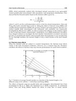
Jure Ravnik and Leopold
ˇ
Skerget
University of Maribor, Faculty of Mechanical Engineering
Slovenia
1. Introduction
Development of numerical techniques for simulation of fluid flow and heat transfer has a long

standing tradition. Computational fluid dynamics has evolved to a point where new methods
are needed only for special cases. In this chapter we introduce a Fast Boundary Element
Method (BEM), which enables accurate prediction of vorticity fields. Vorticity field is defined
as a curl of the velocity field and is an important quantity in wall bounded flows. Vorticity
is generated on the walls and diffused and advected into the flow field. Using BEM, we are
able to accurately predict boundary values of vorticity as a part of the nonlinear system of
equations, without the use of finite difference approximations of derivatives of the velocity
field. The generation of vorticity on the walls is important for the development of the flow
field, shear strain, shear velocity and heat transfer.
The developed method will be used to simulate natural convection of pure fluids and
nanofluids. Over the last few decades buoyancy driven flows have been widely investigated.
Cavities under different inclination angles with respect to gravity, heated either differentially

on two opposite sides or via a hotstrip in the centre, are usually the target of research. Natural
convection is used in many industrial applications, such as cooling of electronic circuitry,
nuclear reactor insulation and ventilation of rooms.
Research of the natural convection phenomena started with the two-dimensional approach
and has been recently extended to three dimensions. A benchmark solution for
two-dimensional flow and heat transfer of an incompressible fluid in a square differentially
heated cavity was presented by Davies (1983). Stream function-vorticity formulation was
used. Vierendeels et al. (2001; 2004) and
ˇ
Skerget & Samec (2005) simulated compressible
fluid in a square differentially heated cavity using multigrid and BEM methods. Rayleigh
numbers between Ra

= 10
2
and Ra = 10
7
were considered. Weisman et al. (2001) studied
the transition from steady to unsteady flow for compressible fluid in a 1 : 4 cavity. They
found that the transition occurs at Ra
≈ 2 ×10
5
. Ingber (2003) used the vorticity formulation
to simulate flow in both square and 1 : 8 differentially heated cavities. Tric et al. (2000)
studied natural convection in a 3D cubic cavity using a pseudo-spectra Chebyshev algorithm

based on the projection-diffusion method with spatial resolution supplied by polynomial
expansions. Lo et al. (2007) also studied a 3D cubic cavity under five different inclinations ϑ
=
0
o
,15
o
,30
o
,45
o
,60

o
. They used a differential quadrature method to solve the velocity-vorticity
formulation of Navier-Stokes equations employing higher order polynomials to approximate
differential operators. Ravnik et al. (2008) used a combination of single domain and sub
domain BEM to solve the velocity-vorticity formulation of Navier-Stokes equations for fluid
Fast BEM Based Methods
for Heat Transfer Simulation
9
2 Heat Transfer
flow and heat transfer.
Simulations as well as experiments of turbulent flow were also extensively investigated. Hsieh
& Lien (2004) considered numerical modelling of buoyancy-driven turbulent flows in cavities

using RANS approach. 2D DNS was performed by Xin & Qu
´
er
´
e (1995) for an cavity with
aspect ratio 4 up to Rayleigh number, based on the cavity height, 10
10
using expansions in
series of Chebyshev polynomials. Ravnik et al. (2006) confirmed these results using a 2D LES
model based on combination of BEM and FEM using the classical Smagorinsky model with
Van Driest damping. Peng & Davidson (2001) performed a LES study of turbulent buoyant
flow in a 1 : 1 cavity at Ra

= 1.59 · 10
9
using a dynamic Smagorinsky model as well as the
classical Smagorinsky model with Van Driest damping.
Low thermal conductivity of working fluids such as water, oil or ethylene glycol led to the
introduction of nanofluids. Nanofluid is a suspension consisting of uniformly dispersed and
suspended nanometre-sized (10–50 nm) particles in base fluid, pioneered by Choi (1995).
Nanofluids have very high thermal conductivities at very low nanoparticle concentrations
and exhibit considerable enhancement of convection (Yang et al., 2005). Intensive research in
the field of nanofluids started only recently. A wide variety of experimental and theoretical
investigations have been performed, as well as several nanofluid preparation techniques have
been proposed (Wang & Mujumdar, 2007).

Several researchers have been focusing on buoyant flow of nanofluids. Oztop & Abu-Nada
(2008) performed a 2D study of natural convection of various nanofluids in partially heated
rectangular cavities, reporting that the type of nanofluid is a key factor for heat transfer
enhancement. They obtained best results with Cu nanoparticles. The same researchers
(Abu-Nada & Oztop, 2009) examined the effects of inclination angle on natural convection
in cavities filled with Cu–water nanofluid. They reported that the effect of nanofluid on heat
enhancement is more pronounced at low Rayleigh numbers. Hwang et al. (2007) studied
natural convection of a water based Al
2
O
3
nanofluid in a rectangular cavity heated from

below. They investigated convective instability of the flow and heat transfer and reported
that the natural convection of a nanofluid becomes more stable when the volume fraction
of nanoparticles increases. Ho et al. (2008) studied effects on nanofluid heat transfer due to
uncertainties of viscosity and thermal conductivity in a buoyant cavity. They demonstrated
that usage of different models for viscosity and thermal conductivity does indeed have
a significant impact on heat transfer. Natural convection of nanofluids in an inclined
differentially heated square cavity was studied by
¨
Og
¨
ut (2009), using polynomial differential
quadrature method. Stream function-vorticity formulation was used for simulation of

nanofluids in two dimensions by G
¨
umg
¨
um & Tezer-Sezgin (2010).
Forced and mixed convection studies were also performed. Abu-Nada (2008) studied the
application of nanofluids for heat transfer enhancement of separated flows encountered in
a backward facing step. He found that the high heat transfer inside the recirculation zone
depends mainly on thermophysical properties of nanoparticles and that it is independent
of Reynolds number. Mirmasoumi & Behzadmehr (2008) numerically studied the effect of
nanoparticle mean diameter on mixed convection heat transfer of a nanofluid in a horizontal
tube using a two-phase mixture model. They showed that the convective heat transfer

could be significantly increased by using particles with smaller mean diameter. Akbarinia
& Behzadmehr (2007) numerically studied laminar mixed convection of a nanofluid in
horizontal curved tubes. Tiwari & Das (2007) studied heat transfer in a lid-driven differentially
heated square cavity. They reported that the relationship between heat transfer and the
volume fraction of solid particles in a nanofluid is nonlinear. Torii (2010) experimentally
210
Heat Transfer - Mathematical Modelling, Numerical Methods and Information Technology
Fast BEM Based Methods for Heat Transfer Simulation 3
studied turbulent heat transfer behaviour of nanofluid in a circular tube, heated under
constant heat flux. He reported that the relative viscosity of nanofluids increases with
concentration of nanoparticles, pressure loss of nanofluids is slightly larger than that of pure
fluid and that heat transfer enhancement is affected by occurrence of particle aggregation.

Development of numerical algorithms capable of simulating fluid flow and heat transfer has
a long standing tradition. A vast variety of methods was developed and their characteristics
were examined. In this work we are presenting an algorithm, which is able to simulate 3D
laminar viscous flow coupled with heat transfer by solving the velocity-vorticity formulation
of Navier-Stokes equations using fast BEM. The velocity-vorticity formulation is an alternative
form of the Navier-Stokes equation, which does not include pressure. The unknown field
functions are the velocity and vorticity. In an incompressible flow, both are divergence free.
Daube (1992) pointed out that the correct evaluation of boundary vorticity values is essential
for conservation of mass. Thus, the main challenge of velocity-vorticity formulation lies
in the determination of boundary vorticity values. Several different approaches have been
proposed for the determination of vorticity on the boundary. Wong & Baker (2002) used
a second-order Taylor series to determine the boundary vorticity values explicitly. Daube

(1992) used an influence matrix technique to enforce both the continuity equation and the
definition of the vorticity in the treatment of the 2D incompressible Navier-Stokes equations.
Liu (2001) recognised that the problem is even more severe when he extended it to three
dimensions. Lo et al. (2007) used the differential quadrature method. Sellountos & Sequeira
(2008) proposed a hybrid multi BEM scheme in combination with local boundary integral
equations and radial basis functions for 2D fluid flow.
ˇ
Skerget et al. (2003) proposed the usage
of single domain BEM to obtain a solution of the kinematics equation in tangential form for the
unknown boundary vorticity values and used it in 2D. This work was extended into 3D using
a linear interpolation in combination with FEM by
ˇ

Zuni
ˇ
c et al. (2007) and using quadratic
interpolation by Ravnik et al. (2009a) for uncoupled flow problems.
The BEM uses the fundamental solution of the differential operator and the Green’s theorem
to rewrite a partial differential equation into an equivalent boundary integral equation. After
discretization of only the boundary of the problem domain, a fully populated system of
equations emerges. The number of degrees of freedom is equal to the number of boundary
nodes. This reduction of the dimensionality of the problem is a major advantage over the
volume based methods. Fundamental solutions are known for a wide variety of differential
operators (Wrobel, 2002), making BEM applicable for solving a wide range of problems.
Unfortunately, integral equations of nonhomogeneous and nonlinear problems, such as heat

transfer in fluid flow, include a domain term. In this work, we solve the velocity-vorticity
formulation of incompressible Navier-Stokes equations. The formulation joins the Poisson
type kinematics equation with diffusion advection type equations of vorticity and heat
transport. These equations are nonhomogenous and nonlinear. In order to write discrete
systems of linear equations for such equations, matrices of domain integrals must be
evaluated. Such domain matrices, since they are full and unsymmetrical, require a lot of
storage space and algebraic operations with them require a lot of CPU time. Thus the domain
matrices present a bottleneck for any BEM based algorithm effectively limiting the maximal
usable mesh size through their cost in storage and CPU time.
The dual reciprocity BEM (Partridge et al. (1992), Jumarhon et al. (1997)) is one of the
most popular techniques to eliminate the domain integrals. It uses expansion of the
nonhomogenous term in terms of radial basis functions. Several other approaches that

enable construction of data sparse approximations of fully populated matrices are also
211
Fast BEM Based Methods for Heat Transfer Simulation
4 Heat Transfer
known. Hackbusch & Nowak (1989) developed a panel clustering method, which also enables
approximate matrix vector multiplications with decreased amount of arithmetical work. A
class of hierarchical matrices was introduced by Hackbusch (1999) with the aim of reducing
the complexity of matrix-vector multiplications. Bebendorf & Rjasanow (2003) developed
an algebraic approach for solving integral equations using collocation methods with almost
linear complexity. Methods based on the expansion of the integral kernel (Bebendorf, 2000)
have been proposed as well. Fata (2010) proposed treatment of domain integrals by rewriting
them as a combination of surface integrals whose kernels are line integrals. Ravnik et al. (2004)

developed a wavelet compression method and used it for compression of single domain BEM
in 2D. Compression of single domain full matrices has also been the subject of research of
Eppler & Harbrecht (2005).
The algorithm proposed in this chapter tackles the domain integral problem using two
techniques: a kernel expansion method based single domain BEM is employed for fast
solution of the kinematics equation and subdomain BEM is used for diffusion-advection type
equations.
In the subdomain BEM (Popov et al., 2007), integral equations are written for each subdomain
(mesh element) separately. We use continuous quadratic boundary elements for the
discretization of function and discontinuous linear boundary element for the discretization
of flux. By the use of discontinuous discretization of flux, all flux nodes are within boundary
elements where the normal and the flux are unambiguously defined. The corners and edges,

where the normal is not well defined, are avoided. The singularities of corners and edges were
dealt with special singular shape functions by Ong & Lim (2005) and by the use of additional
nodes by Gao & Davies (2000). By the use of a collocation scheme, a single linear equation is
written for every function and flux node in every boundary element. By using compatibility
conditions between subdomains, we obtain an over-determined system of linear equations,
which may be solved in a least squares manner. The governing matrices are sparse and have
similar storage requirements as the finite element method. Subdomain BEM was applied on
the Laplace equation by Ram
ˇ
sak &
ˇ
Skerget (2007) and on the velocity-vorticity formulation of

Navier-Stokes equations by Ravnik et al. (2008; 2009a).
The second part of the algorithm uses fast kernel expansion based single domain BEM. The
method is used to provide a sparse approximation of the fully populated BEM domain
matrices. The storage requirements of the sparse approximations scale linearly with the
number of nodes in the domain, which is a major improvement over the quadratic complexity
of the full BEM matrices. The technique eliminates the storage and CPU time problems
associated with application of BEM on nonhomogenous partial differential equations.
The origins of the method can be found in a fast multipole algorithm (FMM) for particle
simulations developed by Greengard & Rokhlin (1987). The algorithm decreases the amount
of work required to evaluate mutual interaction of particles by reducing the complexity of
the problem from quadratic to linear. Ever since, the method was used by many authors for
a wide variety of problems using different expansion strategies. Recently, Bui et al. (2006)

combined FMM with the Fourier transform to study multiple bubbles dynamics. Gumerov
& Duraiswami (2006) applied the FMM for the biharmonic equation in three dimensions.
The boundary integral Laplace equation was accelerated with FMM by Popov et al. (2003).
In contrast to the contribution of this paper, where the subject of study is the application
of FMM to obtain a sparse approximation of the domain matrix, the majority of work done
by other authors dealt with coupling BEM with FMM for the boundary matrices. Ravnik
et al. (2009b) compared wavelet and fast data sparse approximations for boundary - domain
212
Heat Transfer - Mathematical Modelling, Numerical Methods and Information Technology
Fast BEM Based Methods for Heat Transfer Simulation 5
integral equations of Poisson type.
2. Governing equations

In this work, we will present a numerical algorithm and simulation results for heat transfer in
pure fluids and in nanofluids. We present the governing equations for nanofluids, since they
can be, by choosing the correct parameter values, used for pure fluids as well. We assume the
pure fluid and nanofluid to be incompressible. Flow in our simulations is laminar and steady.
Effective properties of the nanofluid are: density ρ
nf
, dynamic viscosity μ
nf
, heat capacitance
(c
p
)

nf
, thermal expansion coefficient β
nf
and thermal conductivity k
nf
, where subscript nf is
used to denote effective i.e. nanofluid properties. The properties are all assumed constant
throughout the flow domain. The mass conservation law for an incompressible fluid may be
stated as

∇·


v = 0. (1)
Considering constant nanofluid material properties and taking density variation into account
within the Boussinesq approximation we write the momentum equation as
∂

v
∂t
+(

v ·

∇)


v = −β
nf
(T −T
0
)

g −
1
ρ
nf


∇
p +
μ
nf
ρ
nf
∇
2

v. (2)
We assume that no internal energy sources are present in the fluid. We will not deal with high
velocity flow of highly viscous fluid, hence we will neglect irreversible viscous dissipation.

With this, the internal energy conservation law, written with temperature as the unknown
variable, reads as:
∂T
∂t
+(

v ·

∇)T =
k
nf
(ρc

p
)
nf
∇
2
T. (3)
Relationships between properties of nanofluid to those of pure fluid and pure solid are
provided with the models. Density of the nanofluid is calculated using particle volume
fraction ϕ and densities of pure fluid ρ
f
and of solid nanoparticles ρ
s

as:
ρ
nf
=(1 − ϕ)ρ
f
+ ϕρ
s
(4)
The effective dynamic viscosity of a fluid of dynamic viscosity μ
f
containing a dilute
suspension of small rigid spherical particles, is given by Brinkman (1952) as

μ
nf
=
μ
f
(1 − ϕ)
2.5
. (5)
The effective viscosity is independent of nanoparticle type, thus the differences in heat transfer
between different nanofluids will be caused by heat related physical parameters only. The heat
capacitance of the nanofluid can be expressed as (Khanafer et al., 2003):
(ρc

p
)
nf
=(1 − ϕ)(ρc
p
)
f
+ ϕ(ρc
p
)
s
. (6)

Similarly, the nanofluid thermal expansion coefficient can be written as
(ρβ)
nf
=(1 −
ϕ)(ρβ)
f
+ ϕ(ρβ)
s
, which may be, by taking into account the definition of ρ
nf
in equation
(4), written as:

β
nf
= β
f
⎡
⎣
1
1 +
(1−ϕ)ρ
f
ϕρ
s

β
s
β
f
+
1
1 +
ϕ
1−ϕ
ρ
s
ρ

f
⎤
⎦
. (7)
213
Fast BEM Based Methods for Heat Transfer Simulation