Heat Transfer Mathematical Modelling Numerical Methods and Information Technology Part 9 pptx

Introduction to Nanoscale Thermal Conduction 5
To understand the effects of a periodic interatomic potential acting on the electron waves,
consider a simple, yet effective, model for the potential experienced by the electrons in a
periodic lattice. This model, the Kronig-Penny Model, assumes there is one electron inside
a square, periodic potential with a period distance equal to the interatomic distance, a,
mathematically expressed as
V
=

0 for 0
< z ≤b
V
0
for −c ≤ z ≤0
, (11)
subjected to the periodicity requirement given by V
(z + b + c)=V(z), where a = b + c.
Solutions of Eq. 10 subjected to Eq. 11 are
ψ
=

D
1
exp[iMz]+D
2
exp[−iMz] for 0 < z ≤ b
D
3
exp[iLz]+D
4
exp[−iLz] for −c ≤ z ≤ 0

, (12)
where D
1
, D
2
, D
3
, and D
4
are constants determined from boundary conditions,

=
¯h
2
M
2
2m
, (13)
and
V
− =
¯h
2
L
2
2m
, (14)
with M and L related to the electron energy.
Although the full mathematical derivation of the predicted allowed electron energies will not
be pursued here (see, for example, Griffiths (2000)), one important part of this formalism is

recognizing that the periodicity in the lattice gives rise to a periodic boundary condition of the
wavefunction, given by
ψ
(z +(b + c)) = ψ(z) exp[iz(b + c)] = ψ( z) exp[ik a], (15)
where k is called the wavevector. Equation 15 is an example of the Bloch Theorem. The
wavevector is defined by the periodicity of the potential (i.e., the lattice), and therefore, the
goal is to determine the allowed energies defined in Eq. 13 as a function of the wavevector. The
relationship between energy and wavevector, 
(k), known as the dispersion relation, is the
fundamental relationship needed to determine all thermal properties of interest in nanoscale
thermal conduction.
After incorporating the Bloch Theorem and continuity equations for boundary conditions of
Eq. 12 and making certain simplifying assumptions (Chen, 2005), the following dispersion
relation is derived for an electron subjected to a periodic potential in a one-dimensional lattice:
A
K
sin
[Mc]+cos[Mc]=cos[kc]. (16)
Here, A is related to the electron energy and atomic potential V, and from Eq. 13
M
=

2m
¯h
2
, (17)
such that Eq. 16 becomes
A

¯h

2
2m
sin


2m
¯h
2
c

+ cos


2m
¯h
2
c

= cos[kc]. (18)
309
Introduction to Nanoscale Thermal Conduction
6 Heat Transfer
Note that the right hand side of Eq. 18 restricts the solutions of the left hand side to only exist
between -1 and 1. However, the left hand side of Eq. 18 is a continuous function that does
in fact exist outside of this range. An energy-wavevector combination that results in the left
hand side of Eq. 18 to evaluating to a number outside of the range from [-1,1] means that an
electron cannot exist for that energy-wavevector combination, indicating that electrons can
only exist at very specific energies related to the interatomic potential between the atoms in
the crystalline lattice. In addition, there is periodicity in the solution to Eq. 18 that arises on
an interval of k

= 2π/c. If the interatomic potential is symmetric, then b = c = 2a, and the
periodicity arises on a length scale of k
= π/a and is symmetric about k = 0. This length of
periodicity is called a Brillouin Zone and, in a symmetric case as discussed here, only the first
Brillouin Zone from k
= 0tok = π/a need be considered due to symmetry and periodicity.
To simplify this picture, now consider the case where the electrons do not ”see” the crystalline
lattice, i.e., the electrons can be considered free from the interatomic potential. In this case, the
electrons are called free electrons. For free electrons, Eqs. 13 and 14 are identical (L
= M) and
A
= 0, thus Eq. 18 becomes
cos


2m
¯h
2
c

= cos[kc]. (19)
From inspection, the free electron dispersion relation is given by

=
¯h
2
k
2
2m
. (20)

This approach of deriving the free electron dispersion relation given by Eq. 20 is a bit
involved, as the Schr
¨
odinger Equation was solved for some periodic potential, and the result
was simplified to the free electron case by assuming the electrons did not ”feel” any of the
interatomic potential (i.e., V
= 0). A bit more straightforward way of finding this free electron
dispersion relation is to solve the Schr
¨
odinger Equation assuming V
= 0. In this case, the
time-independent version of the Schr
¨
odinger Equation (Eq. 10) is given by
−
¯h
2
2m
∂
2
ψ
∂z
2
−ψ = 0. (21)
This ordinary differential equation is easily solvable. Rearranging Eq. 21 yields
∂
2
ψ
∂z
2

+
2m
¯h
2
ψ = 0. (22)
The solution to the above equation takes the form
ψ
= D
5
exp

−i

2m
¯h
2
z

+ D
6
exp

i

2m
¯h
2
z

, (23)

where the wavevector of this plane wave solution is given by k
=

2m/¯h
2
, which yields
the same dispersion relationship as given in Eq. 20. Note that the dispersion relationship
for a free electron is parabolic ( ∝ k
2
). For every k in the dispersion relation, there are
two electrons of the same energy with different spins. Although this is not discussed in
detail in this development, it is important to realize that since two electrons can occupy the
same energy at a given wavevector k (albeit with different spins), the electron energies are
considered degenerate, or more specifically, doubly degenerate.
310
Heat Transfer - Mathematical Modelling, Numerical Methods and Information Technology
Introduction to Nanoscale Thermal Conduction 7
Although the mathematical development in this work focused on the free electron dispersion,
it is important to note the role that the interatomic potential will have on the dispersion.
Following the discussion below Eq. 18, the potential does not allow certain energy-wavevector
combinations to exist. This manifests itself at the Brillouin zone edge and center as a
discontinuity in the dispersion relation. This discontinuity is called a band gap. In practice, for
electrons in a single band, the dispersion is often approximated by the free electron dispersion,
since only at the zone center and edge does the electron dispersion feel the effect of the
interatomic potential. This is a important consideration to remember in the discussion in
Section 4.
Where the dispersion gives the allowed electronic energy states as a function of wavevector,
how the electrons fill the states defines the material as either a metal or a semiconductor. At
zero temperature, the filling rule for the electrons is that they always fill the lowest energy
level first. Depending on the number of electrons in a given material, the electrons will fill

up to some maximum energy level. This topmost energy level that is filled with electrons at
zero Kelvin is called the Fermi level. Therefore, at zero temperature, all states with energies
less than the Fermi energy are filled and all states with energies greater than the Fermi energy
are empty. The location of the Fermi energy dictates whether the material is a metal or a
semiconductor. In a metal, the Fermi energy lies in the middle of a band. Therefore, electrons
are directly next to empty states in the same band and can freely flow throughout the crystal.
This is why metals typically have a very high electrical conductivity. For this reason, the
majority of the thermal energy in a metal is carried via free electrons. In a semiconductor, the
Fermi energy lies in the middle of the band gap. Therefore, electrons in the band directly
below the Fermi energy are not adjacent to any empty states and cannot flow freely. In
order for electrons to freely flow, energy must be imparted into the semiconductor to case
an electron to jump across the band gap into the higher energy band with all the empty
states. This lack of free flowing electrons is the reason why semiconductors have intrinsically
low electrical conductivity. For this reason, electrons are not the primary thermal carrier in
semiconductors. In semiconductors, heat is carried by quantized vibrations of the crystalline
lattice, or phonons.
3.2 Phonons
A phonon is formally defined as a quantized lattice vibration (elastic waves that can exist only
at discrete energies). As will become evident in the following sections, it is often convenient
to turn to the wave nature of phonons to first describe their available energy states, i.e., the
phonon dispersion relationship, and later turn to the particle nature of phonons to describe
their propagation through a crystal.
In order to derive the phonon dispersion relationship, first consider the equation(s) of motion
of any given atom in a crystal. To simplify the derivation without losing generality, attention is
given to the monatomic one-dimensional chain illustrated in Fig. 2a, where m is the mass of the
atom j, K is the force constant between atoms, and a
1
is the lattice spacing. The displacement
of atom m
j

from its equilibrium position is given by,
u
j
= x
j
− x
o
j
, (24)
where x
j
is the displaced position of the atom, and x
o
j
is the equilibrium position of the atom.
Likewise, considering similar displacements of nearest neighbor atoms along the chain and
311
Introduction to Nanoscale Thermal Conduction
8 Heat Transfer
applying Newtown’s law, the net force on atom m
j
is
F
j
= K

u
j+1
−u
j


+ K

u
j−1
−u
j

. (25)
Collecting like terms, the equation of motion of atom m
j
becomes
m
¨
u
j
= K

u
j+1
−2u
j
+ u
j−1

, (26)
where
¨
u
j

refers to the double derivative of u
j
with respect to time. It is assumed that wavelike
solutions satisfy this differential equation and are of the form
u
j
∝ exp
[
i
(
ka
1
−ωt
)]
, (27)
where k is the wavevector. Substituting Eq. 27 into Eq. 26 and noting the identity cos x
=
2(e
ix
+ e
−ix
) yields the expression
mω
2
= 2K
(
1 −cos
[
ka
1

])
. (28)
Finally, the dispersion relationship for a one-dimensional monatomic chain can be established
by solving for ω,
ω
(k)=2

K
m




sin

1
2
ka
1





. (29)
Just as was the case with electrons, attention is paid only to the solutions of Eq. 29 for
−π/a
1
≤ k ≤ π/a
1

, i.e., within the boundaries of the first Brillouin zone. A plot of the
dispersion relationship for a one-dimensional monatomic chain is shown in Fig. 3a. It is
important to notice that the solution of Eq. 29 does not change if k
= k + 2πN/a
1
, where
D

P
.
PPP
D

P
.
0P0
D
E
M M M M
M M M M
PP
M M
P0
M M
Fig. 2. Schematics representing (a) monatomic and (b) diatomic one-dimensional chains.
Here, m and M are the masses of type-A and type-B atoms, a
1
and a
2
are the respective lattice

constants of the monatomic and diatomic chains, and K is the interatomic force constant.
312
Heat Transfer - Mathematical Modelling, Numerical Methods and Information Technology
Introduction to Nanoscale Thermal Conduction 9
D

 D










:DYHYHFWRUN
$QJXODU)UHTXHQF\Ʒ
'HE\H
5HDO
D

 D











:DYHYHFWRUN
$QJXODU)UHTXHQF\Ʒ
0 P
0 P
.P

.0


VW
%ULOORXLQ=RQH

VW
%ULOORXLQ=RQH
F
Ʒ
N
$FRXVWLF
2SWLFDO
D
E
Fig. 3. (a) Phonon dispersion relationship of a one-dimensional monatomic chain as
presented in Eq. 29. Also plotted is the corresponding Debye approximation. Note that not
only does the Debye approximation over-predict the frequency of phonons near the zone
edge, but it also predicts a non-zero slope, and thus, a non-zero phonon group velocity at the
zone edge. (b) Phonon dispersion relationship of a one-dimensional diatomic chain as

presented in Eq. 35. In the case where M
= m, the dispersion is identical to that plotted in (a),
but is represented in a “zone folded” scheme. The size of the phononic band gap depends
directly on the difference between the atoms comprising the diatomic chain.
N is an integer. This indicates that all vibrational information is contained within the first
Brillouin zone.
A phonon dispersion diagram concisely describes two essential pieces of information required
to describe the propagation of lattice energy in a crystal. First, as is obvious from Eq. 29, the
energy of a given phonon, ¯hω, is mapped to a distinct wavevector, k (in turn, this wavevector
can be related to the phonon wavelength). As might be expected, longer wavelength phonons
are associated with lower energies. Second, the group velocity, or speed at which a “packet”
of phonons propagates, is described by the relationship
v
g
=
∂ω
∂k
, (30)
where v
g
is the phonon group velocity. Additional insight can be gained if focus is turned to
two particular areas of the dispersion relationship: the zone center (k
= 0) and the zone edge
(k
= π/a
1
).
Discussion of phonons at the zone center is referred to as the long-wavelength limit.
Evaluating the limit
lim

k→0
∂ω
∂k
= a
1

K
m
, (31)
and noting that both ω and k equal 0 at the zone center, it is found that
ω
= a

K
m
k
= ck, (32)
where c is the sound speed in the one-dimensional crystal. In this limit, the wavelength of
the elastic waves propagating through the crystal are infinitely long compared to the lattice
spacing, and thus, see the crystal as a continuous, rather than discrete medium.
313
Introduction to Nanoscale Thermal Conduction
10 Heat Transfer
Keeping this in mind, a common simplification can be made when considering phonon
dispersion: the Debye approximation. The Debye approximation was developed under the
assumption that a crystalline lattice could be approximated as an elastic continuum. While
elastic waves can exist across a range of energies in such a medium, all waves propagate at the
same speed. This description exactly mimics the zone center limit described in the previous
paragraph, where phonons with wavelengths infinitely long relative to the lattice spacing
travel at the sound speed within the crystal. Naturally, then, under the Debye approximation,

Eq. 32 holds for phonons of all wavelengths, and hence, all wavevectors. The accuracy of the
Debye approximation depends largely on the temperature regime one is working in. In Fig. 3a,
both the slopes and the values of the Debye and real dispersion converge at the zone center.
As a result, the Debye approximation is most accurate describing phonon transport in the
low-temperature limit, where low energy, low frequency phonons dominate (to be discussed
in Section 5).
At the zone edge, a second limit can be established and evaluated,
lim
k→π/a
∂ω
∂k
= 0, (33)
indicating that phonons at the zone edge do not propagate. In this short wavelength limit, the
wavelengths of the elastic waves in the crystal are equal to twice the atomic spacing. Here,
atoms vibrate entirely out-of-phase with each other, leading to the formation of a standing
wave. Advanced texts address the formation of this standing wave further, noting that at
k
= π/a, the Bragg reflection condition is satisfied (Srivastava, 1990). Consequently, the
coherent scattering and subsequent interference of the incoming wave creates the standing
wave condition.
At this point, discussion has been limited to monatomic crystals. However, many materials
of technological interest (semiconductors in particular) have polyatomic basis sets. Thus,
attention is now given to the diatomic one-dimensional chain illustrated in Fig. 2b. Here, m
is the mass of the “lighter” atom, and M is the mass of the “heavier” atom, such that M
> m.
Due to the diatomic nature of this system, equation(s) of motion must be formulated for each
type of atom in the system,
m
¨
u

j
= K

w
j
−2u
j
+ w
j−1

(34a)
m
¨
w
j
= K

u
j+1
−2w
j
+ u
j

. (34b)
Substituting wavelike solutions to these differential equations and isolating ω
2
yields
ω
2

= K

1
m
+
1
M

±K


1
m
+
1
M

2
−
4
mM
sin
2
ka
2

. (35)
Perhaps the most unique feature of Eq. 35 is that for each wavevector k, two unique values of
ω satisfy the expression. As a result, as the two solutions ω
1

and ω
2
are plotted against each
unique k, two distinct phonon branches form: the acoustic branch, and the optical branch.
The distinction between these branches is illustrated in Fig. 3. At the zone center, in the branch
of lower energy, atoms m
j
and M
j
move in phase with each other, exhibiting the characteristic
sound wave behavior discussed above. Thus, this branch is called the acoustic branch. On
the other hand, in the branch of higher energy, atoms m
j
and M
j
move out of phase with
each other. If these atoms had opposite charges on them, as would be the case in an ionic
314
Heat Transfer - Mathematical Modelling, Numerical Methods and Information Technology
Introduction to Nanoscale Thermal Conduction 11
crystal, this vibration could be excited by an electric field associated with the infrared edge of
visible light spectrum (Srivastava, 1990). As such, this branch is called the optical branch. The
phononic band gap between these branches at the zone edge is proportional to the difference
in atomic masses (and the effective spring constants). In the unique case where m
= M, the
solution is identical to that of the monatomic chain.
Extending the one-dimensional cases described above to two or three dimensions is
conceptually simple, but is often no trivial task. For each atom of the basis set, n equations
of motion will be required, where n represents the dimensionality of the system. Generally,
solutions for the resulting dispersion diagrams will yield n acoustic branches and B

(n −
1) optical branches, where B is the number of atoms comprising the basis. While in
the one-dimensional system above we considered only longitudinal modes (compression
waves), in three-dimensional systems, two transverse modes will exist as well (shear waves
due to atomic displacements in the two directions perpendicular to the direction of wave
propagation). Rigorous treatments of such scenarios are presented explicitly in advanced
solid-state texts (Srivastava, 1990; Dove, 1993).
4. Density of states
A convenient representation of the number of energy states in a solid is through the density
of states formulation. The density of states represents the number of states per unit space
per unit interval of wavevector or energy. For example, the one-dimensional density of states
of electrons represents the number of electron states per unit length per dk or per d in the
Brillouin zone. Similarly, the three dimensional density of states of phonons represents the
number of phonon states per unit volume per dk or per dω in the in the Brillouin zone
(for phonons 
= ¯h ω). The general formulation of the density of states in n dimensions
considers the number of states contained in the n
− 1 space of thickness dk per unit space
L
n
. Consequently, the density of states has units of states divided by length raised to the
n divided by the differential wavevector or energy. For example, the density of states of a
three-dimensional solid considers the number of states contained in the volume represented
by the two-dimensional surface multiplied by the thickness dk per unit volume L
3
, where L
is a length, per dk or d. In this section, the density of states will be derived for one-, two-,
and three-dimensional isotropic solids. The representation of an isotropic solid implies that
periodicity arises on a length scale of k
= π/a and is symmetric about k = 0, as discussed in

the last section. This means, that for the isotropic case considered in this chapter, the total
distance from one Brillouin Zone edge to the other is 2π/a. This general derivation yields a
density of states of the n-dimensional solid per interval of wavevector given by
D
nD
=
(
n-1 surface of n-dimensional space)dk

2π
a

n
L
n
dk
, (36)
or per interval of energy given by
D
nD
=
(
n-1 surface of n-dimensional space)dk

2π
a

n
L
n

d
, (37)
where L
n
is the ”volume” of unit space n. Note that a
n
= L
n
. In practice, the density of states
per interval of energy is more conceptually intuitive and is directly input into expressions for
315
Introduction to Nanoscale Thermal Conduction
12 Heat Transfer
the thermal properties, so the starting point for the examples discussed in the remainder of
this section will be Eq. 37.
This general density of states formulation can then be recast into energy space via the electron
or phonon dispersion relations. This is accomplished by solving the dispersion relation for k.
For example, the electron dispersion relation, given by Eq. 20, can be rearranged as
k
=

2m
¯h
2
, (38)
and from this
∂k
=
1
2


2m
¯h
2

∂. (39)
Similarly, assuming the phonon dispersion relation given by Eq. 32 (i.e., the Debye relation)
yields
k
=
ω
v
g
, (40)
and from this
∂k
=
∂ω
v
g
. (41)
Note that recasting Eq. 37 into energy space via a dispersion relation yields the number of
states per unit L
n
per energy interval. In the remainder of this section, the specific derivation of
the one-, two- and three-dimensional electron and phonon density of states will be presented.
This abstract discussion of the density of states will become much more clear with the specific
examples.
4.1 One-dimensional density of states
The starting point for the density of states of a one-dimensional system, as generally discussed

above, is to consider the number of states in contained in a zero dimensional space multiplied
by dk divided by the one-dimensional space of distance 2π/a. Therefore, the one-dimensional
density of states is given by
D
1D
=
dk

2π
a

Ld
. (42)
From Eq. 39, the one-dimensional electron density of states is given by
D
e,1D
= 2 ×
a
2πLd
1
2

2m
¯h
2

d
=
1
2π


2m
¯h
2

, (43)
where the subscript e denotes the electron system and the factor of 2 in front of the middle
equation arises due to the double degeneracy of the electron states, as discussed in Section 3.1
. From Eq. 41, the one-dimensional phonon density of states is given by
D
p,1D
=
a
2πL¯hdω
¯hdω
v
g
=
1
2πv
g
, (44)
where the subscript p denotes the phonon system. Since a Debye model is assumed, the
phonon group velocity is equal to the speed of sound (i.e., v
g
= c), as discussed in Section 3.2.
316
Heat Transfer - Mathematical Modelling, Numerical Methods and Information Technology
Introduction to Nanoscale Thermal Conduction 13
4.2 Two-dimensional density of states

For the density of states in a two-dimensional (2D) system, the starting point is to consider the
number of states along the surface of a circle with radiusk multiplied by dk divided by the 2D
space of area
(
2π/a
)
2
. Therefore, the 2D density of states is given by
D
2D
=
2πkdk

2π
a

2
L
2
d
. (45)
From Eq. 38 and 39, the 2D electron density of states is given by
D
e,2D
= 2 ×
a
2
(
2π
)

2
L
2
d
2π

2m
¯h
2
1
2

2m
¯h
2

d
=
1
π
m
¯h
2
. (46)
Note that the 2D density of states for electrons is independent of energy. From Eq. 40 and 41,
the 2D phonon density of states is given by
D
p,2D
= 2 ×
a

2
(
2π
)
2
L
2
¯hdω
2π
ω
v
g
¯hdω
v
g
=
ω
πv
2
g
. (47)
where the factor of 2 in front of the middle equation arises due to the second dimension, which
introduces a transverse polarization in addition to the longitudinal polarization, as discussed
in Section 3.2. In the discussions in this chapter, equal phonon velocities and frequencies (i.e.,
dispersions) are assumed for each phonon polarization.
4.3 Three-dimensional density of states
The density of states in three-dimensions (3D) will be extensively used in the remainder of
this chapter to discuss nanoscale thermal processes. Following the previous discussions in
this section, the 3D density of states is formulated by considering the the number of states
contained on the surface of a sphere in k-space multiplied by the thickness of the sphere dk

divided by the 3D space of volume
(
2π/a
)
3
. Therefore, the 3D density of states is given by
D
3D
=
4πk
2
dk

2π
a

3
L
3
d
. (48)
From Eq. 38 and 39, the 3D electron density of states is given by
D
e,3D
= 2 ×
a
3
(
2π
)

3
L
3
d
4π
2m
¯h
2
1
2

2m
¯h
2

d
=
1
2π
2

2m
¯h
2

3
2

1
2

. (49)
From Eq. 40 and 41, the 3D phonon density of states is given by
D
p,3D
= 3 ×
a
3
(
2π
)
3
L
3
¯hdω
4π
ω
2
v
2
g
¯hdω
v
g
=
3ω
2
2π
2
v
3

g
, (50)
where the factor of 3 in front of the middle equation arises due to the three dimensions, which
introduces two additional transverse polarizations along with the longitudinal polarization,
as discussed in Section 3.2.
317
Introduction to Nanoscale Thermal Conduction
14 Heat Transfer
5. Statistical mechanics
The principles of quantum mechanics discussed in the previous two sections give the
allowable energy states of electrons and phonons. However, this development did not discuss
the way in which these thermal energy carriers can occupy the quantum states. The bridge
connecting the allowable and occupied quantum states to the collective behavior of the energy
carriers in a nanosystem is provided by statistical mechanics. Through statistical mechanics,
temperature enters into the picture and physical properties such as internal energy and heat
capacity are defined.
It turns out that the thermal energy carriers in nature divide into two classes, fermions and
bosons, which differ in the way they can occupy their respective density of states. Electrons
are fermions that follow a rule that only one particle can occupy a fully described quantum
state (where there are two quantum states with different spins per energy, as discussed in
Section 3.1). This rule was first recognized by Pauli and is called the Pauli exclusion principle.
In a system with many states and many fermion particles to fill these states, particles first
fill the lowest energy states, increasing in energy until all particles are placed. As previously
discussed in Section 3.1, the highest filled energy is called the Fermi energy, 
F
. Phonons are
bosons and are not governed by the Pauli exclusion principle. Any number of phonons can
fall into exactly the same quantum state.
When a nanophysical system is in equilibrium with a thermal environment at temperature T,
then average occupation expectation values for the quantum states are found to exist. In the

case of electrons (fermions), the occupation function is the Fermi-Dirac distribution function,
given by
f
FD
=
1
exp

−
F
k
B
T

+ 1
, (51)
where k
B
is Boltzmann’s constant (Boltzmann’s constant is k
B
= 1.3807 × 10
−23
JK
−1
). For
phonons (bosons), the corresponding occupation function is the Bose-Einstein distribution
function, given by
f
BE
=

1
exp

¯hω
k
B
T

−1
. (52)
Figure 4a and b show plots of Eqs. 51 as a function of electron energy and 52 as a function
phonon frequency, respectively, for three different temperatures, T
= 10, 500, and 1000K.
Given the distribution of carriers, the number of electrons/phonons in a bulk solid at a given
temperature is defined as
n
e/p
=


D
e/p
f
FD/BE
d, (53)
where the dimensionality of the system is driven by the dimensionality of the density of states
of the electrons or phonons derived in Section 4. The total number of electrons and phonons is
mathematically expressed by Eq. 53. The total number of electrons in a bulk solid is constant
as the Fermi-Dirac distribution only varies between zero and one, as seen in Fig. 4a; this is also
conceptually a consequence of the Pauli exclusion principle previously mentioned. Although

the distribution of electron energies change, the number density stays the same. The phonon
number density, however, which has no restriction on number of phonons per quantum
states, continues to increase with increasing temperature. Note that at low temperatures,
the majority of the phonons exist at low frequencies (low energy/long wavelengths). These
phonons correspond to phonons near the center of the Brillouin zone (k
= 0). As temperature
318
Heat Transfer - Mathematical Modelling, Numerical Methods and Information Technology
Introduction to Nanoscale Thermal Conduction 15
  






¡¡
)
([SHFWDWLRQ9DOXH
.
.
.
H9
     







$QJXODU)UHTXHQF\7UDGV


([SHFWDWLRQ9DOXH
.
.
.
D
E
Fig. 4. (a) Fermi-Dirac and (b) Bose-Einstein expectation values calculated from Eqs. 51 and
52, respectively, for three different temperatures, T
= 10, 500, and 1000K. Note that the
expectations values of the Fermi-Dirac distribution function vary from zero to unity, and
therefore represent the probability of an electron being at a certain energy state.
is increased, the proportion of higher frequency (higher energy/shorter wavelength) phonons
that exist increases; these phonons correspond to phonons that are closer to the Brillouin zone
edge (k
= π/a). With the number of electrons/phonons defined in Eq. 53 and following the
discussion in Section 2, the internal energy of the electron/phonon system is defined as
U
e/p
=


D
e/p
f
FD/BE
d. (54)
Now that the internal energies of the electrons and phonons are defined in terms of the

properties of the individual energy carriers, their correspond heat capacities are given by the
temperature derivative of the internal energies, as discussed in Section 2; that is,
C
=
∂U
∂T
. (55)
The heat capacities of electrons and phonons for one-, two-, and three-dimensional solids will
be studied in the remainder of this section.
5.1 Electron heat capacity
Since the zero temperature state of a free electron gas does not correspond to a zero internal
energy system (i.e., U
(T = 0) = 0)), care must be taken when defining the integration limits
in the calculation of the heat capacity. To begin, the internal energy of the T
= 0 state of a free
electron gas is given by
U
e
(T = 0)=

F

0
D
e
f
FD
d. (56)
319
Introduction to Nanoscale Thermal Conduction

16 Heat Transfer
As temperature increases, the electrons redistribute themselves to higher energy levels and
the internal energy is calculated by considering electrons over all energy states, given by
U
e
(T = 0)=
∞

0
D
e
f
FD
d. (57)
Therefore, the change in internal energy of the electron system given some arbitrary δT is
determined by subtracting Eq. 56 from 57, yielding
δU
e
=
∞

0
(
 − 
F
)
D
e
(δ f
FD

) d. (58)
Following Eq. 55, the electronic heat capacity is given by
C
e
=
∞

0
(
 − 
F
)
D
e
∂ f
FD
∂T
d. (59)
At this point, the various electronic density of states defined in Section 4 will be inserted
into Eq. 59 to study the effects of dimensionality on electronic thermal storage. For
convenience, the electronic heat capacity discussion will be limited to metals since electrons
are the dominant thermal carriers in metals and convenient simplifications in the heat
capacity derivations can be made to elucidate the interesting thermophysics. Mainly, at
low-to-moderate temperatures, the density of states in metals can be considered constant and
evaluated at the Fermi energy. This simplifying assumption means that the density of states
can be taken out of the integral in Eq. 59. Therefore, Eq. 59 can be rewritten as
C
e
= D
e

(
F
)
∞

0
(
 − 
F
)
∂ f
FD
∂T
d
= D
e
(
F
)
∞

0
(
 − 
F
)
2
k
B
T

2
exp

−
F
k
B
T


exp

−
F
k
B
T

+ 1

2
d. (60)
Making the substitution of x
≡ ( −
F
)/(k
B
T), Eq. 60 can be re-expressed as
C
e

= D
e
( = 
F
)k
B
T
2
∞

−

F
k
B
T
x
2
exp(x)
(exp(x)+1)
2
dx. (61)
To simplify this integral, consider the lower bound of
−
F
/(k
B
T). At low to moderate
temperatures, the magnitude of this quantity is very large, meaning that this lower bound
extends to very large negative numbers. Therefore, the lower bound of Eq. 61 can be

approximated as negative infinity, so that Eq. 61 can be recast as
C
e
= D
e
( = 
F
)k
B
T
2
∞

−∞
x
2
exp(x)
(exp(x)+1)
2
dx. (62)
This integral can now be solved exactly. By recognizing that
∞

−∞
x
2
exp(x)
(exp(x)+1)
2
dx =

π
2
3
, (63)
320
Heat Transfer - Mathematical Modelling, Numerical Methods and Information Technology
Introduction to Nanoscale Thermal Conduction 17
the electronic heat capacity is given by
C
e
=
π
2
3
k
2
B
TD
e
( = 
F
). (64)
Now to study the electronic heat capacity of electronic systems with different
dimensionalities, the various electronic densities of states derived in Section 4 just need be
inserted into Eq. 64.
Consider the 3D electron density of states given by Eq. 49. Plugging this into Eq. 64 yields
C
e,3D
=
π

2
3
k
2
B
T
1
2π
2

2m
¯h
2

3
2

1
2
F
=
k
2
B
T
6

2m
¯h
2


3
2

1
2
F
. (65)
To simplify this expression further, consider Eq. 53 for a 3D system of electrons. Since, as
previously mentioned, Eq. 53 is constant for electrons, this expression can be evaluated exactly
at T
= 0 to give analytical expression for the electron number density. At zero temperature,
Eq. 53 for electrons becomes
n
e,3D
=

F

0
D
e,3D
f
FD
(T = 0)d =

F

0
D

e,3D
d =
1
3π
2

2m
¯h
2

3
2

3
2
F
. (66)
and from this, it is apparent that for free electrons in a 3D metallic system

2m
¯h
2

3
2
=
3π
2
n
e,3D


3
2
F
. (67)
Inserting Eq. 67 in 65 yields
C
e,3D
=
π
2
k
2
B
n
e,3D
2
F
T, (68)
showing that for a 3D system of free electrons, the heat capacity is directly related to
the temperature, where the proportionality constant is related to material properties. The
electronic heat capacity of Au is plotted in Fig 5.
To examine the electronic heat capacity of a 2D electronic system, consider the 2D electron
density of states given by Eq. 46. Substituting this 2D density of states into Eq. 64 yields
C
e,2D
=
π
2
3

k
2
B
T
1
π
m
¯h
2
=
πk
2
B
T
3
m
¯h
2
. (69)
Following the development for the 3D heat capacity, Eq. 53 for a 2D system of electrons is
given by
n
e,2D
=

F

0
D
e,2D

f
FD
(T = 0)d =

F

0
D
e,2D
d =
1
π
m
¯h
2

F
. (70)
From this, it is apparent that for free electrons in a 2D metallic system
m
¯h
2
=
πn
e,2D

F
. (71)
321
Introduction to Nanoscale Thermal Conduction

18 Heat Transfer
Inserting Eq. 71 in 69 yields
C
e,2D
=
π
2
k
2
B
n
e,2D
3
F
T, (72)
which has a similar dependence on temperature and material properties as the electronic heat
capacity in 3D.
Finally, for a one-dimensional electronic system, consider the one-dimensional density of
states given by Eq. 43. Plugging this into Eq. 64 yields
C
e,1D
=
π
2
3
k
2
B
T
1

2π

2m
¯h
2

F
=
π
6
k
2
B
T

2m
¯h
2

F
. (73)
The number density of a one-dimensional system of electrons is given by
n
e,1D
=

F

0
D

e,1D
f
FD
(T = 0)d =

F

0
D
e,1D
d =
1
2π

2m
F
¯h
2
. (74)
From this

2m
¯h
2
=
2πn
e,1D
√

F

, (75)
which yields
C
e,1D
=
π
2
k
2
B
n
e,1D
3
F
T, (76)
which is also directly proportional to temperature. As apparent from the derivations of
the electronic heat capacities in different dimensionalities of electron systems, the electronic
heat capacity is always directly related to the temperature, regardless of the electron system
dimension.
5.2 Phonon heat capacity
Unlike electrons (fermions), the zero temperature state of phonons (bosons) does not
correspond to a zero internal energy state (i.e., U
(T = 0) = 0) since at T = 0, the lattice is
not vibrating so phonons do not exist. Therefore, the change in internal energy of the phonon
system given some arbitrary δT is determined by evaluating
δU
p
=
ω
max


0
¯hωD
p
(δ f
BE
) dω. (77)
Following Eq. 55, the phonon heat capacity is given by
C
p
=
ω
max

0
¯hωD
p
∂ f
BE
∂T
dω
=
ω
max

0
¯h
2
ω
2

k
B
T
2
D
p
exp

¯hω
k
B
T


exp

¯hω
k
B
T

−1

2
dω. (78)
Since the Debye assumption is employed for the phonon dispersion in these examples, the
maximum phonon frequency is defined as ω
max
= v
g

π/a
1
.
322
Heat Transfer - Mathematical Modelling, Numerical Methods and Information Technology
Introduction to Nanoscale Thermal Conduction 19
The 3D phonon heat capacity is derived by plugging in the expression for the 3D phonon
density of states (Eq. 50) in Eq. 78 which gives
C
p,3D
=
ω
max

0
¯h
2
ω
2
k
B
T
2
3ω
2
2π
2
v
3
g

exp

¯hω
k
B
T


exp

¯hω
k
B
T

−1

2
dω =
ω
max

0
3¯h
2
ω
4
2π
2
v

3
g
k
B
T
2
exp

¯hω
k
B
T


exp

¯hω
k
B
T

−1

2
dω. (79)
The 3D phonon heat capacity of Au is plotted in Fig. 5 along with the electronic heat capacity.
Note that the phonon system heat capacity approaches a constant values at high temperatures.
This limit of constant phonon heat capacity is called the Dulong and Petit limit. The onset of
this Dulong and Petit limit (i.e., the onset of the constant phonon heat capacity) occurs around
a material property called the Debye temperature. The Debye temperature is approximately

the equivalent temperature in which all phonon modes in a solid are excited; this Debye
temperature concept will be quantified in more detail below. Also, note that at very low
temperatures (T
≈ 1 K), the electron system heat capacity is larger than that of the phonon
system. However, for the majority of the temperature range in which Au is solid (the melting
temperature of gold is about 1,300 K), the phonon heat capacity is several orders of magnitude
larger than that of the electrons. Note also the low temperature trend of the phonon heat
capacity is different than the liner trend in temperature exhibited by the electron system. For
the remainder of this section, the low temperature trends in the phonon heat capacity, and the
effect of dimensionality on this trend, will be explored.
To examine the low temperature trends in phonon heat capacity, it is convenient to make the
variable substitution x
≡ ¯hω/(k
B
T). With this, the 3D phonon heat capacity becomes
C
p,3D
=
3k
4
B
2π
2
v
3
g
¯h
3
T
3

x
max
≡θ
D
/T

0
x
4
exp[x]
(
exp[x] −1
)
2
dx, (80)
where the upper limit is redefined as the Debye temperature, θ
D
, divided by the temperature.
Note that θ
D
= ¯hω
max
/k
B
, which is, as previously conceptually discussed, directly related
to the maximum phonon frequency in a solid. In this low temperature limit, T
 θ
D
and
x

max
−→ ∞, so that the integral in Eq. 80 can be evaluated exactly. Recognizing that
∞

0
x
4
exp[x]
(
exp[x] −1
)
2
dx =
4π
4
15
, (81)
the low temperature heat capacity in a 3D phonon system becomes
C
p,3D
=
2π
2
k
4
B
5v
3
g
¯h

3
T
3
, (82)
showing that for a 3D system of phonons, the heat capacity is directly related to the cube of
the temperature at low temperatures, where the proportionality constant is related to material
properties.
Following a similar derivation for a 2D phonon system, plugging Eq. 47 in Eq. 78 gives
C
p,2D
=
ω
max

0
¯h
2
ω
2
k
B
T
2
ω
πv
2
g
exp

¯hω

k
B
T


exp

¯hω
k
B
T

−1

2
dω =
ω
max

0
¯h
2
ω
3
πv
2
g
k
B
T

2
exp

¯hω
k
B
T


exp

¯hω
k
B
T

−1

2
dω. (83)
323
Introduction to Nanoscale Thermal Conduction
20 Heat Transfer
   









7HPSHUDWXUH.
'+HDW&DSDFLW\-NJ

.


(OHFWURQ
3KRQRQ
Fig. 5. 3D electron and phonon heat capacities of Au calculated from Eq. 68 and 80,
respectively. For these calculations, the Au material parameters are assumed as
n
e,3D
= 5.9 × 10
28
m
−3
, 
F
= 5.5 eV = 8.811 ×10
−19
J, and v
g
= 3, 240ms
−1
.
Making the above mentioned x-substitution yields
C
p,2D

=
k
3
B
piv
2
g
¯h
2
T
2
θ
D
/T

0
x
3
exp[x]
(
exp[x] −1
)
2
dx, (84)
As with the 3D case, at low temperatures, the integration can be extended to infinity.
Recognizing that
∞

0
x

3
exp[x]
(
exp[x] −1
)
2
dx = 6ζ[3], (85)
where ζ
[3] is the Zeta function evaluated at 3, the low temperature heat capacity in a 2D
phonon system becomes
C
p,2D
=
6ζ[3]k
3
B
πv
2
g
¯h
2
T
2
, (86)
showing that for a 2D system of phonons, the heat capacity is directly related to the square of
the temperature at low temperatures, where the proportionality constant is related to material
properties.
324
Heat Transfer - Mathematical Modelling, Numerical Methods and Information Technology
Introduction to Nanoscale Thermal Conduction 21

Following a above derivations, the heat capacity of a one-dimensional phonon system is
derived by plugging Eq. 44 in Eq. 78 which gives
C
p,1D
=
ω
max

0
¯h
2
ω
2
k
B
T
2
1
2πv
g
exp

¯hω
k
B
T


exp


¯hω
k
B
T

−1

2
dω =
ω
max

0
¯h
2
ω
2
2πv
g
k
B
T
2
exp

¯hω
k
B
T



exp

¯hω
k
B
T

−1

2
dω. (87)
Making the above mentioned x-substitution yields
C
p,1D
=
k
2
B
2πv
g
¯h
T
θ
D
/T

0
x
2

exp[x]
(
exp[x] −1
)
2
dx, (88)
As with the previous cases, at low temperatures, the integration can be extended to infinity.
Recognizing that
∞

0
x
2
exp[x]
(
exp[x] −1
)
2
dx =
π
2
3
, (89)
the low temperature heat capacity in a one-dimensional phonon system becomes
C
p,1D
=
πk
2
B

6v
g
¯h
T, (90)
showing that for a one-dimensional system of phonons, the heat capacity is directly and
linearly related to the the temperature at low temperatures, where the proportionality constant
is related to material properties. Note that, unlike the electron systems which in which the
temperature trend in heat capacity does not change with dimensionality, an n-dimensional
phonon system has a temperature dependency of T
n
.
6. Thermal conductivity
In the preceding sections, the quantum energy states of electrons and phonons were derived,
and from this, expressions for heat capacities of these thermal energy carriers were presented.
With this, given a particle velocity and scattering time, the thermal conductivity can be
calculated via Eq. 6. In this final section, the thermal conductivity of electrons and phonons
will be calculated from the quantum derivations of heat capacity. The discussion will be
limited to systems in which a 3D density of states can still be assumed and the electrons and
phonons are treated as particles experiencing scattering events, as in the Kinetic Theory of
Gases discussion in Section 2. This approximation of particle transport typical holds true until
characteristic dimensions of nanosystems get below about 10 nm at elevated temperatures
(T
> 50K). Taking the particle approach, and referring to Eq. 6, the thermal conductivity is
given by
κ
e/p
=
1
3
C

e/p,3D
v
2
e/p
τ
e/p
=


D
e/p
∂ f
FD/BE
∂T
v
2
e/p
τ
e/p
d. (91)
As previously discussed, electrons are the dominant thermal carrier in metals where phonons
are the dominant thermal carrier in semiconductors; therefore, the derivation of electron
thermal conductivity will focus on gold for example calculations and the phonon thermal
conductivity calculations will focus on silicon.
325
Introduction to Nanoscale Thermal Conduction
22 Heat Transfer
The final two quantities needed to determine the thermal conductivity of electrons and
phonons are their respective scattering times and velocities. In our particle treatment, the
electrons and phonons can scatter via several different mechanisms, which will be discussed

in more detail later in this section. However, the total scattering rate used in Eq. 91 is related
to the individual scattering processes of each thermal carrier via Matthiessen’s Rule, given by
(Kittel, 2005)
1
τ
=
∑
m
1
τ
m
, (92)
where m is an index representing a specific scattering process of an electron or a phonon.
As for the velocities of the carriers, the phonon velocity was previous defined in Section 3.2,
specifically Eq. 30. Typical phonon group velocities are on the order of v
g
= 10
3
−10
4
ms
−1
.
The electron velocities can be calculated from the Fermi energy. As the electronic thermal
conductivity is related to the temperature derivative of the Fermi-Dirac distribution, only
electrons around the Fermi energy will participate in transport. Approximating all the
electrons participating in transport to have energies of about the Fermi energy, the velocity
of the electrons at the Fermi energy, the Fermi velocity, can be calculated from the common
expression for kinetic energy of a particle so that the electron Fermi velocity is given by
v

F
=

2
F
m
. (93)
Typical Fermi velocities in metals are on the order of 10
6
ms
−1
.
6.1 Electron thermal conductivity
To calculate the thermal conductivity of the electron system via Eq. 91, the final piece of
information that must be known is the electron scattering time. At moderate temperatures,
electrons can lose energy by scattering with other electrons and with the phonons. In metals,
the electron-electron and electron-phonon scattering processes take the form τ
ee
=

A
ee
T
2

−1
and τ
ep
=


B
ep
T

−1
, respectively, where A and B are material dependent constants related
to the electrical resistivity (Kittel, 2005). From Eq. 94, the total scattering time at moderate
temperatures in metals is given by
1
τ
=

1
τ
ee
+
1
τ
ep

= A
ee
T
2
+ B
ep
T. (94)
From this, the electron thermal conductivity is given by
κ
e

=
v
2
F
A
ee
T
2
+ B
ep
T
∞

−∞
( −
F
)D
e,3D
(
F
)
∂ f
FD
∂T
d
=
π
2
k
2

B
n
e,3D
v
2
F
2
F

A
ee
T + B
ep

, (95)
where the simplification on the right hand side comes from the development in Section 5.1.
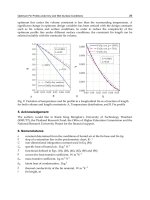
The electron thermal conductivity of Au as a function of temperature predicted via Eq. 95
is shown in Fig. 6a along with the data from Fig. 1. Since the forms of the scattering times
in metals discussed above are only valid for temperatures around and above the Debye
temperature, the thermal conductivity is shown in the range from 100
− 1000 K. Below this
range, additional electron and phonon iterations affect the conductivity that are beyond the
scope of this chapter. The scattering constants, A
ee
and B
ep
are used to fit the model in Eq. 95
326
Heat Transfer - Mathematical Modelling, Numerical Methods and Information Technology
Introduction to Nanoscale Thermal Conduction 23

to the data, and the resulting constants, listed in the figure caption, are in excellent agreement
with previously published values (Ivanov & Zhigilei, 2003). In addition, the temperature
trends agree remarkably well even with the simplified assumptions involved in the derivation
of Eq. 95, showing the power of modeling electron thermal transport from a fundamental
particle level.
With this approach, the effects of nanostructuring on thermal conductivity can now be
calculated. When the sizes of a nanomaterial are on the same order as the mean free path of
the thermal carriers, in the case of metals, the electrons, an additional scattering mechanism
arises due to electron boundary scattering. This boundary scattering time is related to the
length of the limiting dimension, d, in the nanosystem through τ
eb
= d/v
F
. Using this
with Matthiessen’s Rule (Eq. 94), the thermal conductivity of a metallic nanosystem can be
calculated by (Hopkins et al., 2008)
κ
e
=
π
2
k
2
B
n
e,3D
v
2
F
T

2
F

A
ee
T
2
+ B
ep
T +
v
F
d

. (96)
Note that when d is very large, Eq. 96 reduces to Eq. 95. Fig. 6a shows the predicted thermal
conductivity as a function of temperature for Au nanosystems with limiting d indicated in the
figure. Due to electron-boundary scattering, the thermal conductivity of metallic nanosystems
can be greatly reduced by nanostructuring.
6.2 Phonon thermal conductivity
As with the electron thermal conductivity, to calculate the thermal conductivity of the
phonon system via Eq. 91, the phonon scattering times must be known. The major
phonon scattering processes, valid at all temperatures, are phonon-phonon scattering,
phonon-impurity scattering, and phonon-boundary scattering. Note that phonon boundary
scattering exists even in bulk samples since phonons exist as a spectrum of wavelengths,
some of which can be larger than bulk samples. These processes take the form of τ
pp
=

ATω

2
exp
[
−
B/T
]

−1
for phonon-phonon scattering, τ
pi
=

Cω
4

−1
for phonon-impurity
scattering, and τ
pb
=

v
g
/d

−1
for phonon-boundary scattering. Note that this boundary
scattering term represents the bulk boundaries. From this, the total scattering time for
phonons is given by
1

τ
=

1
τ
pp
+
1
τ
pi
+
1
τ
pb

= ATω
2
exp

−
B
T

+ Cω
4
+
v
g
d
. (97)

and the phonon thermal conductivity can be calculated via
κ
e
=
ω
max

0
¯hωD
p,3D
∂ f
BE
∂T
v
2
g

ATω
2
exp

−
B
T

+ Cω
4
+
v
g

d

−1
dω
=
ω
max

0
3¯h
2
ω
4
2π
2
v
g
k
B
T
2
exp

¯hω
k
B
T


exp


¯hω
k
B
T

−1

2

ATω
2
exp

−
B
T

+ Cω
4
+
v
g
d

−1
dω. (98)
where the simplification on the right hand side comes from the development in Section 5.2.
The phonon thermal conductivity of Si as a function of temperature predicted via Eq. 98 is
shown in Fig. 6b along with the data from Fig. 1. The scattering time coefficients A and

327
Introduction to Nanoscale Thermal Conduction
24 Heat Transfer
 


7HPSHUDWXUH.
7KHUPDO&RQGXFWLYLW\:P

.


   




7HPSHUDWXUH.
7KHUPDO&RQGXFWLYLW\:P

.


D$X
E6L
G QP
QP
QP

ƫP

G QP
QP
ƫP
EXONPRGHOGDVKHG
EXONGDWDVROLG
QP
EXONPRGHOGDVKHG
EXONGDWDVROLG
Fig. 6. (a) Electron thermal conductivity of Au as a function of temperature for bulk Au and
for Au nanosystems of various limiting sizes indicated in the plot. The bulk model
predictions, calculated via Eq. 95, are compared to the experimental data in Fig. 1. For these
calculations, A
ee
= 2.4 × 10
7
K
−2
s
−1
and B
ep
= 1.23 × 10
11
K
−1
s
−1
were assumed, in
excellent agreement with literature values (Ivanov & Zhigilei, 2003). Additional
thermophysical parameters used for this calculation are listed in the caption of Fig. 5. The

various Au nanosystem thermal conductivity is calculated via Eq. 96. (b) Phonon thermal
conductivity of Si as a function of temperature for bulk Si and for Si nanoysstems of various
limiting sizes in indicated in the plots. The bulk model predictions, calculated via Eq. 98, are
compared to the experimental data in Fig. 1. For these calculations, the scattering coefficients
were A
= 1.23 × 10
−19
sK
−1
, B = 140K, and C = 1.32 ×10
−45
s
3
. In addition, the group
velocity of Si is taken as the speed of sound, v
g
= 8, 433ms
−1
, and the lattice parameter of Si
is a
= 5.430 × 10
−10
m. To fit the bulk data, d = 8.0 × 10
−3
m. To examine the effects of
nanostructuring, d is varied as indicated in the plot.
B were iterated to match the data after the maximum and C was taken from the literature
(Mingo, 2003). The boundary scattering constant, d, is used as a fitting parameter to match the
data at temperatures lower than the maximum. The resulting coefficients were in excellent
agreement with the literature values for bulk Si (Mingo, 2003). Note that the model using

Eq. 98 fits the data and captures the temperature trends extremely well showing the power
of modeling the bulk phonon thermal conductivity from a fundamental energy carrier level.
To examine the effects of nanostructuring on the phonon thermal conductivity, d is varied
to dimensions indicated in Fig. 6b. Nanostructruing greatly reduces the phonon thermal
conductivity, especially at low temperatures where phonon mean free paths are long.
7. Summary
Modern devices, with feature sizes on the length scale of electron and phonon mean
free paths, require thermal analyses different from that of the phenomenological Fourier
Law. This is due to the fact that the scattering of electrons and phonons in such systems
occurs predominantly at interfaces, inclusions, grain boundaries, etc., rather than within
the materials comprising the device themselves. Here, electrons and phonons have been
described in terms of their respective dispersion diagrams, calculated via the Schr
¨
ordinger
equation for electrons and atomic equations of motion for phonons. Using this information
328
Heat Transfer - Mathematical Modelling, Numerical Methods and Information Technology
Introduction to Nanoscale Thermal Conduction 25
and density of states expressions, energy storage properties, i.e., internal energy and heat
capacity, have been formulated. Lastly, applying the Kinetic Theory of Gases, the thermal
conductivity expressions for metals and semiconductors have been derived. It has been
shown that limiting feature sizes can result in a significant reduction in thermal conductivity.
This, then, once again reinforces the idea that thermal transport on the nanoscale requires an
altogether different approach from that at the macroscale.
8. Acknowledgements
The authors would like to acknowledge Professor Pamela M. Norris at the University of
Virginia for helpful advice and for recommending the writing of this book chapter. P.E.H.
would like to thank Dr. Leslie M. Phinney at Sandia National Laboratories for guidance
and support. P.E.H. is appreciative for funding from the LDRD program office through the
Sandia National Laboratories Harry S. Truman Fellowship Program. J.C.D. is appreciative

for funding from the National Science Foundation Graduate Research Fellowship Program.
Sandia is a multiprogram laboratory operated by Sandia Corporation, a wholly owned
subsidiary of Lockheed Martin Corporation, for the United States Department of Energy’s
National Nuclear Security Administration under Contract DE-AC04-94AL85000.
9. References
Cahill, D. G., Ford, W. K., Goodson, K. E., Mahan, G. D., Majumdar, A., Maris, H. J., Merlin,
R. & Phillpot, S. R. (2003). Nanoscale thermal transport, Journal of Applied Physics
93(2): 793–818.
Chen, G. (2005). Nanoscale Energy Transport and Conversion: A Parallel Treatment of Electrons,
Molecules, Phonons, and Photons, Oxford University Press, New York, New York.
Dove, M. T. (1993). Introduction to Lattice Dynamics, number 4 in Cambridge Topics in Mineral
Physics and Chemistry, Cambridge University Press, Cambridge, England.
Griffiths, D. (2000). Introduction to Quantum Mechanics, 2nd edn, Prentice Hall, Upper Saddle
River, New Jersey.
Ho, C. Y., Powell, R. W. & Liley, P. E. (1972). Thermal conductivity of the elements, Journal of
Physical and Chemical Reference Data 1(2): 279–421.
Hopkins, P. E., Norris, P. M., Phinney, L. M., Policastro, S. A. & Kelly, R. G. (2008). Thermal
conductivity in nanoporous gold films during electron-phonon nonequilibrium,
Journal of Nanomaterials (418050).
Ivanov, D. S. & Zhigilei, L. V. (2003). Combined atomistic-continuum modeling of short-pulse
laser melting and disintegration, Physical Review B 68: 064114.
Kittel, C. (2005). Introduction to Solid State Physics, 8th edn, Wiley, Hoboken, New Jersey.
Mingo, N. (2003). Calculation of Si nanowire thermal conductivity using complete phonon
dispersion relations, Physical Review B 68(11): 113308.
Schr
¨
odinger, E. (1926). Quantisation as a problem of characteristic values, Annalan der Physik
79: 361–376, 489–527.
Srivastava, G. P. (1990). The Physics of Phonons, Adam Hilger, Bristol, England.
Tien, C L., Majumdar, A. & Gerner, F. M. (1998). Microscale Energy Transport, Taylor and

Francis, Washington, D.C.
Vincenti, W. G. & Kruger, C. H. (2002). Introduction to Physical Gas Dynamics, Krieger
Publishing Company, Malabar, Florida.
Wolf, E. L. (2006). Nanophysics and Nanotechnology: An Introduction to Modern Concepts in
329
Introduction to Nanoscale Thermal Conduction
26 Heat Transfer
Nanoscience, 2nd edn, WILEY-VCH Verlag GmbH & Co. KGaA, Weinheim, Germany.
Ziman, J. M. (1972). Principles of the Theory of Solids, 2nd edn, Cambridge University Press,
Cambridge, England.
330
Heat Transfer - Mathematical Modelling, Numerical Methods and Information Technology
14
Study of Hydrodynamics and
Heat Transfer in the Fluidized Bed Reactors
Mahdi Hamzehei
Islamic Azad University, Ahvaz Branch, Ahvaz
Iran

1. Introduction
Fluidized bed reactors are used in a wide range of applications in various industrial
operations, including chemical, mechanical, petroleum, mineral, and pharmaceutical
industries. Fluidized multiphase reactors are of increasing importance in nowadays
chemical industries, even though their hydrodynamic behavior is complex and not yet fully
understood. Especially the scale-up from laboratory towards industrial equipment is a
problem. For example, equations describing the bubble behavior in gas-solid fluidized beds
are (semi) empirical and often determined under laboratory conditions. For that reason
there is little unifying theory describing the bubble behavior in fluidized beds.
Understanding the hydrodynamics of fluidized bed reactors is essential for choosing the
correct operating parameters for the appropriate fluidization regime. Two-phase flows

occur in many industrial and environmental processes. These include pharmaceutical,
petrochemical, and mineral industries, energy conversion, gaseous and particulate pollutant
transport in the atmosphere, heat exchangers and many other applications. The gas–solid
fluidized bed reactor has been used extensively because of its capability to provide effective
mixing and highly efficient transport processes. Understanding the hydrodynamics and
heat transfer of fluidized bed reactors is essential for their proper design and efficient
operation. The gas–solid flows at high concentration in these reactors are quite complex
because of the coupling of the turbulent gas flow and fluctuation of particle motion
dominated by inter-particle collisions. These complexities lead to considerable difficulties in
designing, scaling up and optimizing the operation of these reactors [1-3].
Multiphase flow processes are key element of several important technologies. The presence
of more than one phase raises several additional questions for the reactor engineer.
Multiphase flow processes exhibit different flow regimes depending on the operating
conditions and the geometry of the process equipment. Multiphase flows can be divided
into variety of different flows. One of these flows in gas-solid flows. In some gas-solid
reactors (fluidized reactors); gas is the continuous phase and solid particles are suspended
within this continuous phase. Depending on the properties of the gas and solid phases,
several different sub-regimes of dispersed two-phase flows may exist. For relatively small
gas flow rates, the rector may contain a dense bed of fluidized solid particles. The bed may
be homogenously fluidized or gas may pass through the bed in the form of large bubbles.
Further increase in gas flow rate decreases the bed density and the gas-solid contacting
pattern may change from dense bed to turbulent bed, then to fast-fluidized mode and
ultimately to pneumatic conveying mode. In all these flow regimes the relative importance
Heat Transfer - Mathematical Modelling, Numerical Methods and Information Technology
332
of gas-particle, particle-particle, and wall interaction is different. It is, therefore necessary to
identify these regimes to select an appropriate mathematical model. Apart from density and
particle size as used in Geldart's classification, several other solid properties, including
angularity, surface roughness and composition may also significantly affect quality of
fluidization (Grace, 1992). However, Geldart's classification chart often provides a useful

starting point to examine fluidization quality of a specific gas-solid system. Reactor
configuration, gas superficial velocity and solids flux are other important parameters
controlling the quality of fluidization. At low gas velocity, solids rest on the gas distributor
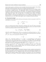
and the regime is a fixed bed regime. The relationship between some flow regimes, type of
solid particles and gas velocity is shown schematically in Fig.1. When superficial gas
velocity increases, a point is reached beyond which the bed is fluidized. At this point all the
particles are just suspended by upward flowing gas. The frictional force between particle
and gas just counterbalances the weight of the particle.


Fig. 1. Progressive change in gas-solid contact (flow regimes) with change on gas velocity
This gas velocity at which fluidization begins is known as minimum fluidization velocity
(
m
f
U
) the bed is considered to be just fluidized, and is referred to as a bed at minimum
fluidization. If gas velocity increases beyond minimum fluidization velocity, homogeneous
(or smooth) fluidization may exist for the case of fine solids up to a certain velocity limit.
Beyond this limit (
mb
U
: minimum bubbling velocity), bubbling starts. For large solids, the
bubbling regime starts immediately if the gas velocity is higher than minimum fluidization
velocity (U
mb
= U
mf
). With an increase in velocity beyond minimum bubbling velocity, large
instabilities with bubbling and channeling of gas are observed. At high gas velocities, the

movement of solids becomes more vigorous. Such a bed is called a bubbling bed or
Study of Hydrodynamics and Heat Transfer in the Fluidized Bed Reactors
333
heterogeneous fluidized bed, in this regime; gas bubbles generated at the distributor
coalesce and grow as they rise through the bed. For deep beds of small diameter, these
bubbles eventually become large enough to spread across the diameter of the vessel. This is
called a slugging bed regime. In large diameter columns, if gas velocity increases still
further, then instead of slugs, turbulent motion of solid clusters and voids of gas of various
size and shape are observed, Entrainment of solids becomes appreciable. This regime is
called a turbulent fluidized bed regime. With further increase in gas velocity, solids
entrainment becomes very high so that gas-solid separators (cyclones) become necessary.
This regime is called a fast fluidization regime. For a pneumatic transport regime, even
higher gas velocity is needed, which transports all the solids out of the bed. As one can
imagine, the characteristics of gas-solid flows of these different regimes are strikingly
different. It is, therefore, necessary to determine the prevailing flow regime in order to select
an appropriate mathematical model to represent it.
Computational fluid dynamics (CFD) offers an approach to understanding the complex
phenomena that occur between the gas phase and the particles. With the increased
computational capabilities, computational fluid dynamics (CFD) has become an important
tool for understanding the complex phenomena that occur between the gas phase and the
particles in fluidized bed reactors [3, 4, 5]. As a result, a number of computational models
for solving the non-linear equations governing the motion of interpenetrating continua that
can be used for design and optimization of chemical processes were developed. Two
different approaches have been developed for application of CFD to gas–solid flows,
including the fluidized beds. One is the Eulerian-Lagrangian method where a discrete
particle trajectory analysis method based on the molecular dynamics model is used which is
coupled with the Eulerian gas flow model. The second approach is a multi-fluid Eulerian–
Eulerian approach which is based on continuum mechanics treating the two phases as
interpenetrating continua. The Lagrangian model solves the Newtonian equations of motion
for each individual particle in the gas-solid system along with a collision model to handle

the energy dissipation caused by inelastic particle-particle collision. The large number of
particles involved in the analysis makes this approach computationally intensive and
impractical for simulating fluidized bed reactors at high concentration. The Eulerian model
treats different phases as interpenetrating and interacting continua. The approach then
develops governing equations for each phase that resembles the Navier-Stokes equations.
The Eulerian approach requires developing constitutive equations (closure models) to close
the governing equations and to describe the rheology of the gas and solid phases.
For gas-solid flows modeling, usually, Eulerian-Lagrangian are called discrete particle
models and Eulerian-Eulerian models are called granular flow models. Granular flow
models (GFM) are continuum based and are more suitable for simulating large and complex
industrial fluidized bed reactors containing billions of solid particles. These models,
however, require information about solid phase rheology and particle-particle interaction
laws. In principle, discrete particle models (DPM) can supply such information. DPMs in
turn need closure laws to model fluid-particle interactions and particle-particle interaction
parameters based on contact theory and material properties. In principle, it is possible to
work our way upwards from direct solution of Navier-Stokes equations. Lattice-Boltzmann
models and contact theory to obtain all the necessary closure laws and other parameters
required for granular flow models. However, with the present state of knowledge, complete
a priori simulations are not possible. It is necessary to use these different models judiciously.
Combined with key experiments, to obtain the desired engineering information about