MIMO Systems Theory and Applications Part 4 pot

Semi-Deterministic Single Interaction MIMO Channel Model

95
where
'
x
E and
'
y
E
are the x and y components of the reflected electric field from wall5.
The same procedure is applicable for other walls. To find Γ
TM
and Γ
TE
, angles of incidence
and transmission are required [Wentworth, 2005]:


⎪
⎪
⎩
⎪
⎪
⎨
⎧
θη+θη
θη−θη
=Γ
θη+θη

θη−θη
=Γ
)
i
cos(
1
)
t
cos(
2
)
i
cos(
1
)
t
cos(
2
TM
)
t
cos(
1
)
i
cos(
2
)
t
cos(

1
)
i
cos(
2
TE
(18)
where (
η
1
, η
2
), (θ
i
, θ
t
) are the intrinsic impedances of free space and wall material and angles
of incidence and transmission, respectively. Referring to Fig. 5, one can easily calculate
angles of incidence and transmission for wall5 as follows:

⎪
⎪
⎩
⎪
⎪
⎨
⎧
θ
=θ
−

π
=θ
2
k
)
i
sin(
1
k
arcsin
t
5
A
5
B
Rx
h
arctan
2
i
(19)
where (θ
i
, θ
t
), h
Rx
, (k
1
, k

2
) are angles of incidence and transmission, Rx height and wave
number of air and wall material, respectively.
3.4 Channel capacity calculation
Assuming that the channel is unknown to the transmitter and the total transmitted power is
equally allocated to all
N
T
antennas, the capacity of the system is given by [Foschini & Gans,
1998]:

2
*
T
SNR
C=lo
g
(det[ + × ] )
N
norm(HH )
⎛⎞
⎡
⎤
⎜⎟
⎢
⎥
⎜⎟
⎢
⎥
⎣

⎦
⎝⎠
T
*
N
HH
I
bps/Hz (20)
where
T
N
I is

the

identity matrix, SNR is the average signal to noise ratio within the receiver
aperture, N
T
is the number of transmitter antennas, H is the N
T
×N
R
channel matrix and H*
is the conjugate transpose of
H. To calculate H-matrix baseband channel complex impulse
response should be computed for scatterers, reflectors and direct path corresponding to each
channel.
1.
Scatterers

(
)
]
eff
)
bs
r(E
eff
)
bs
r(E[
s
N
1q
sqb
r
msq
r
)
sqb
r
msq
r(jk
e
scatterers
h
ϕ
⋅
ϕ
+

θ
⋅
θ
=
×
+−
=
∑
A
G
G
A
G
G
GG
G
G
(21)
where )
eff
,
eff
(),E,E(,
sqb
r,
msq
r,
s
N
ϕθ

ϕθ
A
G
A
G
G
G
are the number of scatterers, distance vector
from Tx (MS) to q
th
scatterer, distance vector from Rx (BS) to q
th
scatterer, effective radiation
pattern at Rx in
θ
a
G
and
φ
a
G
directions (radiation patterns of Tx and Rx are included in
effective radiation pattern), and effective lengths of the half-wavelength dipole in
θ
a
G
and
φ
a
G

directions, respectively.
MIMO Systems, Theory and Applications

96
Assuming that the half-wavelength dipole antenna is connected to a matched load and
current distribution is sinusoidal, two components of effective complex length of dipole can
be obtained from [Collin, 1985]:

⎪
⎪
⎩
⎪
⎪
⎨
⎧
ϕ
π
λ
=
ϕ
θ
π
λ
=
θ
0
E
E
eff
0

E
E
eff
A
G
A
G
(22)
where
θ
E
and
φE
are the electric fields radiated by the half-wavelength dipole while it is
in transmitting mode.
2.
Reflectors

(
)
]
eff
)
br
r(E
eff
)
br
r(E[
r

N
1q
rqb
r
mrq
r
)
rqb
r
mrq
r(jk
e
reflectors
h
ϕ
⋅
ϕ
+
θ
⋅
θ
=
×
+−
=
∑
A
G
G
A

G
G
GG
G
G
(23)
where )
eff
,
eff
(),E,E(,
rqb
r,
mrq
r,
r
N
ϕθ
ϕθ
A
G
A
G
G
G
are the number of reflectors, distance vector
from Tx to
q
th
reflector (wall), distance vector from Rx to q

th
reflector, effective radiation
pattern at Rx in
θ
a
G
and
φ
a
G
directions, and effective lengths of the half-wavelength dipole in
θ
a
G
and
φ
a
G
directions, respectively.
3.
Direct Path
To obtain direct field between Tx and Rx, the following equation is used:

mb
-jk r
direct θ bm effθ jbm eff
mb
e
[E (r ) E (r ) ]
r

=⋅+⋅
G
G
G
GG
AA
G
h
ϕ
(24)
where
mb eff eff
r,(E,E),( , )
θφ θ φ
G
G
G
AA
are the distance vector from Tx to Rx, effective radiation pattern
at Rx in
θ
a
G
and
φ
a
G
directions and the effective lengths of the half-wavelength dipole in
θ
a

G

and
φ
a
G
directions, respectively.
3.5 Coordinate transformations
To find the total electric field at Rx which is the last destination of the traveled wave, many
coordinate transformations should be performed. Since, it is much easier to transform
rectangular coordinates of local and global systems rather than spherical ones, before each
transformation step, electric field in rectangular coordinate should be found.
Equation (25) is used frequently while developing the mathematical model. It is a general
formula to rotate a coordinate system and convert it to the other one by knowing the angles
between their axes.

N
N
1 112131 1
2 122232 2
31323333
__
_
ˆ ˆˆˆˆˆˆ ˆ
ˆ ˆˆˆˆˆˆ ˆ

ˆ ˆˆˆˆˆˆ ˆ

New S
y

stem Old S
y
stem
Rotation Matrix
u auauau a
u auauau a
uauauaua
⎡
⎤⎡⋅ ⋅ ⋅⎤⎡⎤
⎢
⎥⎢ ⎥⎢⎥
=⋅ ⋅ ⋅
⎢
⎥⎢ ⎥⎢⎥
⎢
⎥⎢ ⎥⎢⎥
⋅⋅⋅
⎣
⎦⎣ ⎦⎣⎦
(25)
Semi-Deterministic Single Interaction MIMO Channel Model

97
The given solution in (7) is for an x oriented field propagation along the z-axis. However,
these conditions will rarely be met since the same coordinate system is used for all
scatterers. By employing a local coordinate system for each object, the mentioned solution
can be applied.
Different local and global coordinates are shown in Fig. 6 and defined as follows:
•
Gmain (x

Gmain
, y
Gmain
, z
Gmain
) is the global coordinate.
•
G1

(x
G1
, y
G1
, z
G1
) is a parallel coordinate system with Gmain and its origin is on the
center of Tx.
•
L1 (x
L1
, y
L1
, z
L1
) is the local coordinate for Tx antenna and its origin is the same as that
of G1 and also for this coordinate system z
L1
is chosen along the direction of Tx dipole
and x
L1

is defined on the plane of x
G1
and y
G1
.
•
L2 (x
L2
, y
L2
, z
L2
) is the local coordinate for scatterers and its origin is on the scatterer
center and for this coordinate system
z
L2
is chosen along the direction of r
L1
and x
L2
is
chosen along the direction of
1L
θ
ˆ
. r
L1
, θ
L1
, φ

L1
are spherical coordinate components of
each scatterer in respect to
L1 coordinate. It is worth mentioning that for each scatterer
an
L2 coordinate is defined.
•
L3 (x
L3
, y
L3
, z
L3
) is the local coordinate for Rx antenna the origin of which is on the
center of Rx and also for this coordinate system z
L3
is chosen along the direction of Rx
dipole and
x
L3
is defined on a plane parallel to the plane of x
Gmain
and y
Gmain
.


Fig. 6. Global and local coordinates and dipole antennas at both ends.
The local coordinates L1 and L3 are defined to provide the possibility of using different
polarizations for Tx and Rx antennas, respectively.

Now to fulfill the condition required for using the scattering formulas, L1 coordinate system
should be converted to L2 coordinate system which is the local coordinate system of each
scatterer. If the scatterer is located at (r
L1
, θ
L1
, φ
L1
) in respect to L1 coordinate system, to
convert L1 into L2 coordinates system, one can use:

11 1 11
11 1 11
2
11
cos cos sin sin cos
ˆˆ ˆˆ
ˆˆ
cos sin cos sin sin
sin 0 cos
LL L LL
LL L LL
LL1
LL
xyz xyz
θϕ ϕ θϕ
θϕ ϕ θϕ
θθ
−
⎡

⎤
⎢
⎥
=
⎡⎤⎡⎤
⎣⎦⎣⎦
⎢
⎥
⎢
⎥
−
⎣
⎦
(26)
MIMO Systems, Theory and Applications

98
where θ
L1
and φ
L1
are scatterer’s coordinates referring to L1.
If the Tx antenna type is something other than dipole or generally, is an antenna with
electric field in both θ
ˆ
and
φ

directions then the relation between the L1 and L2 coordinate
systems is more complicated and the corresponding rotation matrix is as follows:

[][]
⎥
⎥
⎥
⎦
⎤
⎢
⎢
⎢
⎣
⎡
θθ
ϕ
+θ
θ
−
ϕθϕ
θ
+ϕθ
ϕ
−ϕ
ϕ
+ϕθ
θ
ϕθϕ
θ
−ϕθ
ϕ
−ϕ
ϕ

−ϕθ
θ
××=
1L
cosA
1L
sinE
1L
sinE
1L
sin
1L
sinA
1L
cosE
1L
sin
1L
cosE
1L
cosE
1L
sin
1L
cosE
1L
cos
1L
sinA
1L

sinE
1
L
cos
1L
cosE
1L
sinE
1L
cos
1L
cosE

A
1

1L
z
ˆ
y
ˆ
x
ˆ
2L
z
ˆ
y
ˆ
x
ˆ

(27)
where E
θ
, E
φ
are the electric field components at each scatterer center referred to L1 and θ
L1

and φ
L1
are scatterer’s coordinates and
22
θφ
A= E +E . Equation (27) is simplified to rotation
matrix in (26) if Tx antennas has electric field only in
θ direction.
Finally, after all conversions of coordinate systems, the vectors which are necessary to find
channel complex impulse response such as electric fields and effective lengths should be
converted to the main global coordinate which is specified as G
main
in Fig. 6.
4. Verifying the SISTER model
To verify the obtained results from developed model, “Wireless Insite” software by Remcom
Inc. [Remcom Inc., 2004] is used. This software is a three-dimensional ray tracing tool for
both indoor and outdoor applications which models the effects of surrounding objects on
the propagation of electromagnetic waves between Tx and Rx.
In order to accomplish this verification, different steps have been taken. First, only a direct
path between Tx and Rx is considered for a Single Input Single Output (SISO) system and
received power is verified by both Friis equation and ray tracing tool.
It is assumed that a half wavelength dipole antenna (Gain=2.16dBi) is used at both ends, Tx-

Rx distance is 2.7m, both Tx and Rx heights are 1.5m and transmitted power is 0dBm
(1mW). For the mentioned system configuration, numerical results obtained from both
proposed mathematical model and ray tracing are summarized in Table 1.


P
received
|E
z
| (V/m) Phase E
z
(degree)

SISTER Model
-44.362 dBm
(3.663×10
-8
W)
0.117 76.917
Ray Tracing
-44.350 dBm
(3.673×10
-8
W)
0.117 73.496
Friis Equation
-44.337dBm
(3.684×10
-8
W)

Table 1. Numerical results for a SISO system.
As it can be seen the result obtained from the SISTER model matches well with a fractional
error less than 0.006 with both ray tracing tool and also Friis transmission equation given in
(28) [Balanis, 1997]:
Semi-Deterministic Single Interaction MIMO Channel Model

99

t
G
r
G
2
)
R4
(
t
P
r
P
π
λ
= (28)
where P
r
, P
t
, λ, R, G
r

and G
t
are received power, transmitted power, wavelength, Tx-Rx
distance and Rx and Tx antenna gains, respectively.
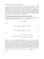
In the next step (Fig. 7) one wall is added to the previous system configuration and the
reflected ray is evaluated as well. For this case, summarized results can be found in Table 2
which again shows an acceptable match with those of the ray tracing. The same procedure
to validate the reflected field has been done for all six walls and all have shown good match.


Fig. 7. Ray tracing visualization of a SISO system in an indoor environment considering
reflection from one wall.


P
received
|E
z
| (V/m) Phase E
z
(degree)

SISTER Model
-48.442 dBm
(1.432×10
-8
W)
0.073 -115.719
Ray Tracing
-48.461 dBm

(1.425×10
-8
W)
0.073 -121.210
Table 2. Numerical results for a SISO system configuration shown in Fig. 7
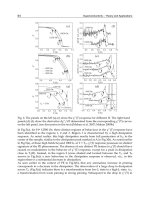
Channel capacity for the MIMO system configuration illustrated in Fig. 8 is compared for
both proposed model and ray tracing tool. Fig. 9 shows the results for three cases; direct
path only, reflected paths only, total paths.


Fig. 8. Ray tracing visualization of a 4×4-MIMO system in an indoor environment
considering six walls.
MIMO Systems, Theory and Applications

100
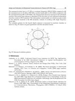
As the final step to verify the results, the capacity of MIMO systems with different N
T
×N
R

antenna numbers are evaluated in an outdoor environment for NLOS case and the results
are compared with Rayleigh model for similar antenna numbers. Fig. 10 shows the
capacities obtained from simulated Rayleigh channel by MATLAB and SISTER model
applied to an outdoor NLOS environment with 30 scatterers for different numbers of
antennas.
As these results show good agreement with both ray tracing tool and Rayleigh model is
achieved.


Fig. 9. Comparing MIMO channel capacity obtained from SISTER model and ray tracing tool

for different rays.
0 5 10 15 20 25 30
0
2
4
6
8
10
13
14
SNR (dB)
Capacity (bps/Hz)
Outdoor Channel Capacity for Different MIMO Element Numbers (NLOS)
SISTER 4*2
SISTER 2*4
SISTER 2*2
SISTER 1*1
Rayleigh 2*2
Rayleigh 2*4

Fig. 10. Comparing channel capacity obtained from SISTER model and Rayleigh model.
The MIMO configuration is the same as Fig.8 and the room dimensions are 5×4×3 m
3
and a
wall exists to block the LOS path.
5. Results of applying SISTER model for different scenaris
Although the SISTER model is sufficiently general to be applied to any distributions and
locations for the scatterers, here we concentrate only on picocell environments.
Semi-Deterministic Single Interaction MIMO Channel Model

101
Moreover, “Angle Diversity” which is a new promising solution and has recently attracted
considerable attention in MIMO system designs [Allen et al., 2004] is also evaluated model
and compared with well-known “Space Diversity” method by applying the SISTER. In this
method, instead of multiple antennas used in space diversity case, multiple simultaneous
beams are assumed at both sides. The main advantage of this technique comparing is that it
allocates high capacity not to all the points in space, but the desired ones. This results in
minimum undesired interference. The main difficulty in such systems, however, is the beam
cusps (beam overlaps) [Allen & Beach, 2004] and finding the optimal angles where the
different beams should be directed towards. We have investigated the use of antenna array
in angle diversity case to implement the narrow beams needed in this method. We also have
addressed some problems with beam cusps which introduce correlations in MIMO
channels, and suggested some solutions to overcome this problem.
Here, various results are presented which are ultimately useful to set the system design
parameters and to evaluate and compare the performance of MIMO systems using space or
angle diversity for both outdoor and indoor environments. Due to space limitations only some
of the results are presented here and more results can be found in [E.Forooshani, 2006].
5.1 SISTER results for outdoor environments
Outdoor system specifications considered are summarized in Table 3. Tx refers to
transmitter and Rx refers to receiver antennas. Without loosing the generality, it is assumed
that mobile set (MS) is the transmitter and the base station (BS) is the receiver side. All
simulations are done based on working frequency of 2.4GHz. For results shown in Figs 11-
15, a 4×4 MIMO system is considered.
Two common scatterer distributions for outdoor environments are uniform distribution
around each end and cluster distribution, as shown in Fig. 11(a) and Fig. 11(b), respectively.


Tx (MS)
height
Rx (BS) height

Relative hei
g
ht of Tx and
Rx
Distance between
Tx and Rx
Outdoor
System
24
λ (3m) 40λ (5m) 16λ (2m) 102λ (13m)
Table 3. Outdoor system specifications.


Fig. 11. Outdoor system configuration for: (a) NLOS scenario with uniformly distributed
scatterers around both ends, (b) LOS scenario with cluster form scatterers in a cubic volume
(200
λ×150λ×50λ or 25×18.75×6.25, m
3
).
MIMO Systems, Theory and Applications

102
5.1.1 Impact of ground material
For outdoor environment, impact of two types of ground material, high and low conductive
ones (Fig. 12) are investigated. Reflection from the high conductive ground contributes as
much as the direct path and its presence can suppress the effect of direct path and hence
increase the capacity comparing to the low conductive ground case. It also shows that for a
ground with conductivity more than 100 S/m, capacity is mainly controlled by the reflected
path from the ground and scatterers do not contribute much in the channel capacity.

Fig. 12. Channel capacity at signal to noise ratio, SNR=30dB for different ground materials
(
ε
r
=4, ε
r
=25) considering 30 uniformly distributed scatterers, the LOS case.
5.1.2 Impact of number of scatterers
Figs. 13 and 14 show the impact of number of uniformly distributed scatterers in terms of
channel capacity versus SNR. Typical number of scatterers for this study is 30. In NLOS
case, it is assumed that there is no direct path but reflection from the ground exists (blocked
LOS or quasi-LOS). Fig. 13 shows the LOS case. In this case reflection from the high
conductive ground contributes as much as the direct path. Therefore, its presence can
suppress the effect of direct path and hence increase the capacity in compare to the low
conductive ground case.
For NLOS case, shown in Fig. 14, when the number of scatterer is not high (30 scatterers)
reflection from the high conductive ground creates the dominant path and capacity is low.
When the number of scatterers is high enough (100 scatterers), they are able to lessen the
effect of reflection from the ground and in this case capacity is higher. For low conductive
ground, on the other hand, the reflection from the ground is so weak that no dominant path
exists and hence for both cases of 30 and 100 scatterers, channel capacity is high.
5.1.3 Comparing space and angle diversities
To compare space and angle diversity methods for a 4×4-MIMO system, a scenario
consisting of four clusters of scatterers is considered. The length occupied by antenna
elements is the same for both space and angle diversity methods. It is essential to keep the
array length the same if we intend to have a fair comparison between the two methods in
terms of system size and length. Antenna array length at both ends is 1.5
λ.
Direct Path

Direct Path
+Reflection
Semi-Deterministic Single Interaction MIMO Channel Model

103
For space diversity case, four antenna elements are used while in angle diversity the same
four elements are used along with a Butler matrix to create four simultaneous beams with
different scan angles. Assumptions made for space and angle diversity methods are
summarized in Table 4.




Fig. 13. Channel capacity for different number of scatterers distributed uniformly around
both ends in LOS case (
σ=ground’s electrical conductivity, S/m).




Fig. 14. Channel capacity for different numbers of scatterers distributed uniformly around
both ends in NLOS case including reflection from the ground but not the direct path
(
σ=ground’s electrical conductivity).
σ =∞
σ = 0.001
σ = ∞
σ = 0.001
MIMO Systems, Theory and Applications

104

Number of
elements at
BS
Number of
elements at
MS
BS element
spacing (
d-Rx)
MS element
spacing (d-Tx)
Space Diversity 4 4 0.5λ 0.5λ
Angle Diversity 4 4 0.5λ 0.5λ
Table 4. Assumptions for space and angle diversity methods.
For space and angle diversities channel capacity is calculated based on equations (29) and
(30), respectively.

2
T
SNR
C(SNR)=lo
g
(det[ + × ])
N
norm( )
⎛⎞
⎡
⎤

⎜⎟
⎢
⎥
⎜⎟
⎢
⎥
⎣
⎦
⎝⎠
T
*
N
*
HH
I
HH
(29)

2TxRx
T
SNR
C(SNR)=lo
g
( det[ +(G ×G ) × ])
N
norm( )
⎛⎞
⎡
⎤
⎜⎟

⎢
⎥
⎜⎟
⎢
⎥
⎣
⎦
⎝⎠
T
*
N
*
HH
I
HH
(30)
where C is the channel capacity,
T
N
I is the Identity matrix, SNR is the signal to noise ratio,
N
T
is number of transmitter antennas (or beams) and H is the channel matrix, whose
elements are calculated using the SISTER model. For space diversity h
ij
is the path gain
between antenna element
i at BS and j at MS. For angle diversity each h
ij
represents the path

gain between
i
th
beam at BS and j
th
beam at MS.
Factor (G
Tx
× G
Rx
) in (30) shows the array gain of angle diversity method. When an array
consists of elements with the spacing of 0.5
λ, then its gain is equal to the number of elements
if antenna losses are ignored (G
Tx
× G
Rx
=4×4=16). Since it is assumed that the total power is
the same for two systems, it is required to take the array gain into account while comparing
capacities of two methods in terms of SNR. Note that no mutual coupling effect is assumed
in this calculation.
Fig.15 shows four beams angels at MS and BS sides for angle diversity case.


(a) (b)
Fig. 15. Four multibeams which are pointed towards four clusters located in different
θ
angles (a) MS (Tx) (N-array=4, beam angles=62
o
, 70

o
, 91
o
, 105
o
), (b) BS (Rx) (N-array=4, beam
angles=60
o
, 83
o
, 117
o
, 132
o
).
Semi-Deterministic Single Interaction MIMO Channel Model

105
Table 5 and Fig. 18 (a) show singular values of normalized H-matrix and capacity results for
both methods in LOS case, respectively. Table 6 and Fig. 16 (b) show singular values of
normalized
H-matrix and capacity results for both methods in NLOS case, respectively.
As Fig. 16 show angle diversity surpass space diversity significantly, mostly due to the array
gain. Even though angle diversity often shows better channel orthogonality, improperly
chosen angles caused not to achieve the maximum available capacity for the angle diversity.

Singular Value1 Singular Value2 Singular Value3 Singular Value4
Space Div. 1.0000 0.0016 0.0004 0.0000
Angle Div. 1.0000 0.0024 0.0008 0.0000
Table 5. Singular values for 30 scatterers in 4 clusters for LOS.

Singular Value1 Singular Value2 Singular Value3 Singular Value4
Space Div. 1.0000 0.4424 0.0062 0.0003
Angle Div. 1.0000 0.4481 0.0007 0.0000
Table 6. Singular values for 30 scatterers in 4 clusters for NLOS.
For NLOS case, the rays from Tx towards clusters behind the block are stopped which cause
reduction in the number of channels. Another reason which has caused getting undesirable
results for angle diversity method in both LOS and NLOS cases is the beam cusps.
Considering above discussion, for the given scenario, angle diversity seems to be an
appropriate alternative for space diversity which can provide similar orthogonality with less
interference.


(a) (b)
Fig. 16. Channel capacity for 30 scatterers in 4 clusters for (a) LOS, (b) NLOS.
5.1.4 Impact of number of clusters
The impact of the number of clusters on the channel capacity for a NLOS scenario, similar to
what was shown in Fig. 11(b) is also studied. To consider the effects of number of clusters,
clusters in this configuration are located in such a way to avoid blockage by the defined
obstacle in the middle of the study area. Fig. 17 shows that for a certain amount of SNR, as
MIMO Systems, Theory and Applications

106
the number of clusters increases, at first, channel capacity increases but after a while it
remains constant. This is expected as by increasing the number of clusters multipath
components are increased and correlation between channels is decreased. However, after a
certain point the slope of capacity increase decreases because as the space is limited the
clusters are going to be closer to each other and after a while they will have overlaps. This
reduces the orthogonality of the channels. These results are also in agreement with those
cited in [Burr, 2003] based on “finite scatterer channel model” Also note that as the number

of scatters increases and the spacing between them decreases due to the increase in mutual
interactions a single interaction models such as SISTER is not accurate anymore.


Fig. 17. Channel capacity at SNR=30 dB for different numbers of clusters which contain 10
scatterers each.
5.2 SISTER results for indoor environments
5.2.1 Office area
In order to characterize the indoor channel, the outdoor model is enhanced in such a way
that it includes not only the scatterers and reflection from the ground but also reflection
from the walls for a typical office area of 5×4×3 m
3
. Indoor system specifications considered
in this study are summarized in Table 7.


Tx
height
Rx
height
Relative
height of
Tx and
Rx
Distance
between
Tx and
Rx
Room’s
dimension

Scatterers’
radius
Scatterers’
number
Office
10.4λ
(1.3m)
14.4λ
(1.8m)
4λ (0.5m)
32.24λ
(4.3m)
5×4×3(m
3
) 0.1m 30
Table 7. A typical office area specifications.
Two distributions of uniform and cluster form for scatterers are considered to study an
office area (Fig. 18).
Semi-Deterministic Single Interaction MIMO Channel Model

107




Fig. 18. An office area including Tx, Rx and 30 scatterers distributed (a) uniformly and (b) in
cluster form.
5.2.2 Comparing space and angle diversities
Space and angle diversities are compared for different scenarios in [E.Forooshani, 2006] but
only results for 30 uniformly distributed and cluster scatterers in indoor are presented here.

Selected antenna beams in 2×2-MIMO angle diversity were (62
o
, 121
o
) for Tx and (72
o
, 119
o
)
for Rx. In 4×4-MIMO systems beams were selected at (48
o
, 65
o
, 130
o
, 138
o
) for both sides.
Capacities of both systems are shown in Fig. 19.
The composition of singular values is also given in Table 8. The results show that for the
4×4-MIMO system for both LOS and NLOS cases, angle diversity surpasses space diversity
method in terms of channel orthogonality. Moreover, it offers array gain which leads in an
increase in the capacity shown in Fig. 19(b). Based on these results, for this system, it is more
convenient to apply angle diversity method since LOS and NLOS capacities are similar if the
beams are selected properly while this is not true for space diversity. Furthermore, applying
angle diversity helps to lessen the interference effects (compare to omnidirectional antennas,
MIMO Systems, Theory and Applications

108
the power is directed to limited angles) in an indoor environment which is a real concern

nowadays.
By try and error, it was found that, particularly for LOS case, higher capacity can be
achieved by choosing angles far away from the direct path which in most cases is
approximately around horizontal plane (
θ=90
o
).
In the 2×2-MIMO for space diversity, instead of 4 elements, there are 2 elements at each end
with the spacing of 3
λ/2 and for angle diversity; there are two arrays with λ spacing
between array centers. Each array consists of 2 dipoles with
λ/2 spacing.
To study angle diversity method for this 2×2-MIMO system in LOS case where 30 scatterers
are uniformly distributed, two beams are directed towards the reflecting points of ceiling
and the floor which actually are the two angles far from the direct path. For NLOS case,



Fig. 19. Capacity for (a) 2×2-MIMO and (b) 4×4-MIMO systems.

SV1 SV2 SV3 SV4
Space Div. (LOS) 4×4-MIMO 1.0000 0.0067 0.0008 0.0000
Angle Div. (LOS) 4×4-MIMO 1.0000 0.1120 0.0011 0.0005
Space Div. (NLOS) 4×4-MIMO 1.0000 0.0208 0.0087 0.0002
Angle Div. (NLOS) 4×4-MIMO 1.0000 0.2252 0.0658 0.0000
Space Div. (LOS) 2×2-MIMO 1.0000 0.0094
Angle Div. (LOS) 2×2-MIMO 1.0000 0.1529
Space Div. (NLOS) 2×2-MIMO 1.0000 0.0011
Angle Div. (NLOS) 2×2-MIMO 1.0000 0.1816
Table 8. Comparing singular values for the 2×2-MIMO and 4×4-MIMO systems (SV:

Singular Value).
Semi-Deterministic Single Interaction MIMO Channel Model

109
however, since no direct path exists, there is more freedom to find the desirable angles.
Therefore, different angles for the NLOS case are chosen for beams that one of them is not
that far from the horizontal plane.
In practical application, even though it would not be feasible to perform angle optimization
every time there is a change in the Tx and Rx position, there is a possibility to develop a
method for finding optimum angles. In the systems that reference signals are used even
infrequently, the initial optimization based on these signals can be done and followed by
updates by estimating the Angle of Arrival (AOA). The assumption in this work was that
receiver has no information about the channel. This means beamforming methods that need
temporal and spatial reference (training signals) is not applicable. In that case semi-blind
adaptive beamforming techniques can be utilized to find the optimum angles [Allen &
Ghavami, 2005]. Main concern in this work can be if the angle diversity with non-optimum
angles can still outperform space diversity. Therefore, angles were chosen heuristically and
no optimization was performed to find the best possible ones. The results show, for the 2×2-
MIMO system similar to what was obtained for the 4×4-MIMO system, angle diversity
works better for both LOS and NLOS cases. Although angle diversity for 4×4-MIMO system
shows better performance, still 2×2-MIMO system gives desirable results. If one uses
beamforming techniques more desirable results might be achieved.
Space and angle diversity methods are also compared for office area where scatterers are in
cluster form. First beam angles were chosen based on the clusters’ location and they were
(61
o
, 77
o
, 103
o

, 121
o
). It can be noted that these beams are very close to each other and have
some cusps. These cusps cause increase in the correlation among the channels and show
decrease in channel capacity, therefore they were changed in such a way that have less cusp
(43
o
, 73º, 108
o
, 136
o
), but they were not directed to clusters any more. This improved the
capacity. The capacity results for both sets are given in Fig. 20. In general cluster location
can give a good guide to find the beam angles and then by considering the cusps between
beams and blockage by walls a correction should be applied to improve the capacity.




Fig. 20. Channel capacity for 30 scatterers in cluster form in the 4×4-MIMO system.
MIMO Systems, Theory and Applications

110
6. Conclusion
In this chapter a mathematical model to characterize wireless communication channel is
developed which falls into semi-deterministic channel models. This model is based on
electromagnetic scattering and reflecting and fundamental physics however it has been kept
simple through appropriate assumptions.
Based on the results obtained from the SISTER model, impact of different factors on the
channel capacity were studied for different scenarios which represent possible wireless

MIMO systems such as Wireless Local Area Networks (WLAN) systems in real outdoor and
indoor environments. Performance of space and angle diversity methods in MIMO systems
are also compared and evaluated. Some of the main achievements are as follows.
The results obtained by SISTER model confirms that higher capacities are achieved for
NLOS cases compare to LOS or quasi-LOS cases. However, in LOS or quasi-LOS cases
where there is a single dominant path which introduces correlation among the MIMO
channels, strong path’s dominancy can be lessened by another strong path obtained from
either a strong reflection or a resultant path of large number of scatterers and hence channel
capacity will be improved. A better alternative to space diversity to improve the channel
capacity (especially for LOS case) is the use of angle diversity method. This technique is a
promising solution in MIMO systems whose main advantage is to allocate high capacity not
to all the points but to the desired ones which results in minimum interference for undesired
areas. Therefore, it can be very attractive for environments where interference is the main
consideration. Probably the main advantage of angle diversity over space diversity is the
similar performance of LOS and NLOS cases, while the space diversity shows a significant
reduction in performance for the LOS case.
For angle diversity method in LOS case, high performance can be achieved by selecting
beams such that they are not close to horizontal plane where usually a direct path exists. In
fact, in LOS cases nulls of the beams should be directed towards the direct path between Tx
and Rx to create decorrelated channels.
Even though angle diversity often shows better channel orthogonality, improperly chosen
angles lessen the probability of obtaining the maximum achievable capacity. Therefore,
choosing the right angles is very important. Improper selection can degrade the
performance of a 4×4-MIMO system to that one of a 2×2-MIMO system. In general locations
of clusters of scatterers can give a good guide to find the beam angles. However, after the
initial selection correction has to be done to avoid beam cusps and blockage by walls. This is
because the beam cusps can degrade the capacity due to increase correlation between
channels. Based on this study, only in some scenarios, angle diversity shows better
performance in LOS cases compare to NLOS as some scatterers which can be those with
high contributions on channel orthogonality are blocked. Consequently, for most scenarios,

angle diversity seems to be an appropriate alternative for space diversity which can provide
similar orthogonality with less interference. Even if in some cases it shows less
orthogonality still better performance than space diversity can be achieved because of
higher SNR due to the array gain.
7. References
Allen, B. & Beach, M. (2004). On the analysis of switched beam antennas for the WCDMA
downlink,
IEEE Trans. Veh. Technol., Vol. 53, No. 3, (2004), pp. 569-578.
Semi-Deterministic Single Interaction MIMO Channel Model

111
Allen, B.; Brito, R.; Dohler, M. & Aghvami, H. (2004). Performance comparison of spatial
diversity array technologies,
IEEE Trans. Consum. Electron., Vol. 50, No. 2, (2004),
pp. 420-428.
Allen B. & Ghavami M. (2005).
Adaptive Array Systems: Fundamentals and Applications, John
Wiley & Sons, Inc., 978-0-470-86189-9, NY, USA.
Almers P.; Bonek E.; Burr A.; Czink, N.; Debbah M.; Degli-Esposti V.; Hofstetter H.; Kyosti
P.; Laurenson D.; Matz G.; Molisch A. F.; Oestges C. & H. O¨ zcelik H. (2007).
Survey of channel and radio propagation models for wireless MIMO systems,
EURASIP J. Wirel. Commun. Netw., pp. 1-19, (2007).
Anderson, C.R. & Rappaport, T.S. (2004). In-building wideband partition loss measurements
at 2.5 and 60 GHz,
IEEE Trans. Wirel. Commun. Vol. 3, No. 3, (2004), pp. 922 – 928.
Balanis, C. (1989).
Advanced Engineering Electromagnetics, John Wiley & Sons, Inc., 0-471-
621943, NY, USA.
Balanis, C. (1997). Antenna Theory Analysis and Design, John Wiley & Sons, Inc., 0-471-
59268-4, NY, USA.

Burr, A. G. (2003). Capacity bounds and estimates for the finite scatterers MIMO Wireless
Channel,
IEEE J. Sel. Areas Commun., Vol. 21, No. 5, (2003), pp. 812-818.
Chizhik, D.; Ling, J.; Wolniansky, P.W.; Valenzuela, R.A.; Costa, N. & Huber, K. (2003).
Multiple-input-multiple-output measurements and modeling in Manhattan,
IEEE J.
Sel. Areas Commun., 2003, Vol. 21, No. 3, (2003), pp. 321 – 331.
Collin, R.E. (1985).
Antennas and Radiowave Propagation, McGraw-Hill, NY, USA.
E. Forooshani, A. (2006).
MIMO systems channel modeling and analysis, Master of Science
Thesis, University of Manitoba, Canada.
E. Forooshani, A. & Noghanian, S. (2010). Semi-deterministic channel model for MIMO
systems Part-I: Model development and validation,
IET Microwave Antennas and
Propag.
, Vol. 4, No. 1, (2010), pp. 17-25.
Foschini, J. & Gans, M. (1998). On the limit of wireless communications in a fading
environment when using multiple antennas,
Wirel. Pers. Commun., Vol. 6, No. 3,
(1998), pp. 311-335.
Gesbert, D.; Bolcskei, H.; Gore, D.A. & Paulraj, A.J. (2002). Outdoor MIMO wireless
channels: models and performance prediction,
IEEE Trans. Commun. , Vol. 50,
No.12, (2002), pp. 1926 – 1934.
Howard, S.; Inanoglu, H.; Ketchum, J.; Wallace, M. & Walton, R. (2002). Results from MIMO
channel measurements,
Proc. 13
th
IEEE Symp. Personal Indoor and Mobile Radio

Communications, pp. 1932 – 1936, Lisboa, Portugal, Sept. 2002.
Liberti, J.C. & Rappaport, T.S. (1996). A geometrically based model for line-of-sight
multipath radio channels
, Proc. IEEE 46th, Vehicular Technology Conf., pp. 844 – 848,
Atlanta, GA, 1996.
Liberti J.C. & Rappapaort, T.S. (1999).
Smart Antennas for Wireless Communications, Prentice
Hall, 0137192878, Upper Saddle River, NJ, USA.
Ranvier, S.; Kivinen, J. & Vainikainen, (2007). Millimeter-wave MIMO radio channel
sounder,
IEEE Trans. Instrum. Meas., Vol. 56, No. 3, (2007), pp. 1018 – 1024.
Remcom Inc. Technical Staff (2004).
Wireless Insite, Remcom Inc., version 2.0.5.
MIMO Systems, Theory and Applications

112
Seidel, S.Y. & Rappaport, T.S. (1994). Site-specific propagation prediction for wireless in-
building personal communication system design,
IEEE Trans. Veh. Technol., Vol.
43, No.4, (1994), pp. 879 – 891.
Svantesson, T. (2001).
Antenna and Propagation from a Signal Processing Perspective, PhD
dissertation, Chalmers University of Technology, Sweden.
Wentworth, S.M. (2005).
Fundamentals of Electromagnetics with Engineering Applications, John
Wiley & Sons, 978-0-470-10575-7, 111 River Street, Hoboken,
NJ, USA.
Part 2
Information Theory Aspects

0
Another Interpretation of Diversity
Gain of MIMO Systems
Shuichi Ohno
1
and Kok Ann Donny Teo
2
1
Hiroshima University
2
DSO National Laboratories
1
Japan
2
Singapore
1. Introduction
Multiple-Input Multiple-Output (or the so-called MIMO) system, which employs multiple
antennas at both ends of the receiver and transmitter terminals, has been the subject
of intensive research efforts in the past decade with potential application in high speed
wireless communications network. This is chiefly motivated by the benefits of 1) the spatial
multiplexing gain, which makes use of the degrees of freedom in communication system by
transmitting independent symbol streams in parallel through spatial channels, to improve
bandwidth efficiency; 2) diversity gain, which can be achieved by averaging performance over
multiple path gains to combat fading, to improve channel capacity and/or bit-error rate (BER).
Information theoretical analysis reveals that MIMO systems indeed offer high spectral
efficiency (Foschini, 1996; Goldsmith et al., 2003; Telatar, 1999). It has been shown in (Tse
and Viswanath, 2005) that the capacity of an N
r
× N
t

MIMO system with N
t
transmit and N
r
receive antennas over i.i.d. Rayleigh fading channels scales with the minimum of the number
N
t
of transmit antennas and the number N
r
of receive antennas at the high SNR regime. With
ideal capacity achieving Gaussian codes, capacity is attained by minimum mean squared error
successive interference cancellation (MMSE-SIC) at the receiver (Tse and Viswanath, 2005) if
the number of receive antennas is equal to or larger than the number of transmit antennas.
The receive diversity achieved by endorsing multiple receive antennas have been utilized
in practical communication systems. Recently, Space-Time codes have also been developed
to obtain transmit antenna diversity gain (Alamouti, 1998; Caire and Shamai, 1999; Ma and
Giannakis, 2003; Tarokh et al., 1999; Xin et al., 2003). Performance gains induced by different
schemes of MIMO systems were comprehensively compared in (Catreux et al., 2003).
It is well-known that there is a tradeoff between multiplexing gain and diversity gain.
The diversity gain is usually measured by the slope of the BER curve. Over i.i.d. Rayleigh
distributed channels, the diversity order of N
r
× N
t
systems with linear equalization is given
by N
r
− N
t
+ 1 at high SNR at full multiplexing (Winters et al., 1994). This implies that given a

fixed number N
t
of transmit antennas, increasing the number N
r
of receive antennas increases
the diversity order. Conversely, given a fixed N
r
,anincreaseinN
t
(which contributes to
multiplexing gain) decreases the diversity order. In (Narasimhan, 2003), by exploiting the
5
tradeoff, an adaptive control of the number of transmit antennas and symbol constellations
is proposed to improve the performance of spatial multiplexing in correlated fading channels.
Moreover, theoretical analysis that shows a fundamental tradeoff between multiplexing gain
and/or diversity gain including Vertical-Bell Laboratories Layered Space-Time (V-BLAST)
and Space-Time Codes (STC) have been reported (Tse and Viswanath, 2005; Zheng and Tse,
2003).
Capacity or ergodic capacity, which is the capacity averaged over fading channels, are often
utilized to evaluate capacity gain. On the other hand, BER or average BER, which is the BER
averaged over fading channels, relate to diversity gain. These gains have been analyzed by
approximate expressions for these measures at the SNR extremes, or by directly evaluating
them for a particular channel probability density function (pdf), e.g., i.i.d. complex-normal
distribution (Chiani et al., 2003; Marzetta and Hochwald, 1999; Smith et al., 2003). However,
since the full diversity order appears only at high SNR, having higher diversity order does not
necessarily mean having better performance at a particular value of SNR. Moreover, diversity
gain of Rayleigh channels does not necessarily imply the existence of diversity gain for other
distributed channels. In this chapter, we study universal properties of the performance of
MIMO system as in (Ohno and Teo, 2007), which is independent of channel probability density
functions and hold at any SNR.

We only consider the case where the performance measure is a convex or concave function of
SNR. However, it is shown that important performance measures, including channel capacity
and BER, are convex or concave. Thus, our results are significant. To get more insights into
MIMO systems, we study capacity gain from a different point of view. A similar approach is
adopted in (Ohno and Teo, 2007) to analyze the impact of antenna size of MIMO systems on
BER performance with zero-forcing (ZF) equalization.
Take channel capacity for example. Let us suppose that you can install an additional receive
antenna in the N
r
× N
t
system to construct an (N
r
+ 1) × N
t
system. Assume that the
underlying channel environment is not time-varying (i.e., static). Then, can any other gain
(besides power gain) be obtained by increasing the number of receive antennas? Without the
values of channel coefficients or the associated channel pdf, no one can answer this question
or evaluate the possible gain correctly. Now, we look at the problem from another perspective.
For simplicity, we put N
r
= 2andN
t
= 2. From a 3 × 2 system, we can remove one receive
antenna in three different ways to obtain three possible 2
×2 systems. Then, we compare the
performance of the original 3
× 2 system with the average performance of the three 2 × 2
systems. We show in this chapter that without the knowledge of channel coefficients and at

any value of SNR, the capacity of the original 3
×2 system is greater than the average capacity
of the three 2
×2 systems. More generally, our analysis reveals that increasing the number of
receive antennas generates capacity gain even in static channels. From this, we can prove that
the mean capacity with respect to channel pdf, which is mathematically equivalent to the
so-called ergodic capacity for fading channels, increases as the number of receive antennas
increases at any value of SNR. Our proof relies not on the channel pdf but on the concavity
of the capacity function. This implies that the concavity is indispensable to obtain receive
antenna diversity.
Next, we consider removing a transmit antenna from an N
r
× N
t
system and compare the
capacity of the N
r
× N
t
system with the average capacity of N
r
× (N
t
−1) systems. Clearly,
removing one transmit antenna reduces the multiplexing gain. For comparison, we adopt
the capacity per transmit antenna as a parameter. Then, we prove that reducing the number
116
MIMO Systems, Theory and Applications
of transmit antennas improves the capacity per transmit antenna. It follows that the mean
capacity per transmit antenna degrades as the number of transmit antennas increases at any

value of SNR irrespective of channel pdf. This means that increasing the number of transmit
antennas improves the multiplexing gain but degrades the capacity per transmit antenna.
There exists a tradeoff between multiplexing gain and capacity gain regardless of channel pdf
and SNR.
Although we do not evaluate how much gains there actually are, which requires the
knowledge of channel coefficients or channel pdf, our results are universal in the sense that
performance ordering with the number of transmit antennas and the number of receive
antenna is independent of channel pdf and holds true at any value of SNR. We also study
the achievable information rate of block minimum mean squared error (MMSE) equalization
to obtain similar results.
2. Preliminaries and system model
We consider a MIMO transmission with N
t
transmit and N
r
receive antennas over flat
non-frequency-selective channels. Let us define ρ/N
t
as the transmit power at each transmit
antenna for the N
r
× N
t
MIMO system. We denote the path gain from transmit antenna n
(n ∈ [1, N
t
]) to receive antenna m (m ∈ [1, N
r
]) as h
mn

.Thepathgainsareassumedtobe
unknown to the transmitter but perfectly known to the receiver.
Let the received signal at receive antenna m be x
m
.TheN
r
received signals are arranged in a
vector as x
=[x
1
, ,x
N
r
]
T
,where[·]
T
denotes transposition. Then, x is expressed as
x
=

ρ
N
t
Hs + w,(1)
where the N
r
× N
t
channel matrix H ,theN

t
×1 combined data vector s having i.i.d. entries
with unit variance, the N
r
×1vectorw of zero mean circular complex additive white Gaussian
noise (AWGN) entries with unit variance are respectively given by
H
=
⎡
⎢
⎣
h
11
h
1N
t
.
.
.
.
.
.
.
.
.
h
N
r
1
h

N
r
N
t
⎤
⎥
⎦
,(2)
s
=

s
1
s
N
t

T
,(3)
w
=

w
1
w
N
r

T
.(4)

Let the mth row (which corresponds to the mth receive antenna) of the channel matrix H be
h
m
for m ∈ [1, N
r
],andthenth column (which corresponds to the nth transmit antenna) of the
channel matrix H be
˜
h
n
for n ∈ [1, N
t
] so that we can also express the channel matrix as
H
=
⎡
⎢
⎣
h
1
.
.
.
h
N
r
⎤
⎥
⎦
=


˜
h
1
···
˜
h
N
t

.(5)
The signal-to-noise ratio (SNR) at receive antenna m is found to be ρ
||h
m
||
2
/N
t
,where||·||is
the 2-norm of a vector, while the overall receive power of the symbol transmitted from antenna
n, i.e., the sum of power from transmit antenna n at all receive antennas, is ρ
||
˜
h
n
||
2
/N
t
.

117
Another Interpretation of Diversity Gain of MIMO Systems
With capacity achieving Gaussian codes, for a given channel H, the information rate of the
N
r
× N
t
MIMO system is expressed as (see. e.g. (Telatar, 1999; Tse and Viswanath, 2005))
C
N
r
,N
t
= log




I
N
r
+
ρ
N
t
HH
H





= log




I
N
t
+
ρ
N
t
H
H
H




,(6)
where
(·)
H
stands for complex conjugate transposition. Over fading channels, MIMO system
offers the benefits of multiplexing gain and/or capacity/diversity gain (Larsson and Stoica,
2003; Tse and Viswanath, 2005).
For our analysis that follows, we utilize the achievable information rates of non-linear
Maximum Likelihood (ML) equalization and minimum mean squared error (MMSE)
equalization. MMSE equalizations at the receiver becomes available if the channel matrix has

column full rank, which requires N
r
≥ N
t
.
Let us shortly review MMSE equalization for MIMO systems. If we employ block-by-block
equalization, the MMSE equalizer is given by G
=

ρ
N
t
H
H
(
ρ
N
t
HH
H
+ I
N
r
)
−1
.The
equalized output is thus expressed as ˆs
= Gx.Wedefinethenth entry of the equalized output
as
ˆ

s
n
= p
n
s
n
+ v
n
,wherev
n
is the effective noise contaminating the nth symbol. Then, we can
show that the signal-to-interference noise ratio (SINR) of symbol n after MMSE equalization
is expressed as (Kay, 1993; Tse and Viswanath, 2005)
SINR
N
r
,N
t
,n
=
ρ
N
t
˜
h
H
n

I
N

r
+
ρ
N
t
N
t
∑
l=1,l=n
˜
h
l
˜
h
H
l

−1
˜
h
n
.(7)
Block-by-block MMSE equalization can be easily implemented but cannot achieve the
capacity except for some special cases. Capacity is achieved by MMSE successive interference
cancellation (MMSE-SIC) at the receiver. Then, SIC with optimal cancellation order is utilized
in Vertical-Bell Laboratories Layered Space-Time (V-BLAST) (Foschini et al., 1999). Although
cancellation order affects the BER performance, it does not change the achievable information
rate (Tse and Viswanath, 2005, Chapter 8). Thus, it is convenient in what follows to only
consider the simplest MMSE-SIC that does not perform the optimal ordering (i.e., arbitrary
ordering) procedure. We first equalize symbols from transmit antenna 1. Then after decoding

them, the contribution of the signal due to the symbol from transmit antenna 1 is reconstructed
and eradicated from the received vector. The same procedure is repeated for the remaining
symbols from transmit antenna 2 to transmit antenna N
t
. If we denote the SINR of the
equalized output at the nth step of MMSE-SIC as SINR
SIC
n
and there is no error propagation,
then the capacity in (6) can be adequately expressed as (Tse and Viswanath, 2005, Chapter 8)
C
N
r
,N
t
=
N
t
∑
n=1
log

1 + SINR
SIC
n

.(8)
3. Decreasing the number of receive antennas
Based on the mathematical tools in the previous section, we investigate information rates of
MIMO systems when we decrease the number of receive antennas, while fixing the number of

transmit antennas. As the number of receive antennas decreases/increases, the overall receive
power decreases/increases, which is known as power loss/gain. Thus, it seems obvious that
capacity degrades as the number of receive antennas decreases. However, the MIMO system
118
MIMO Systems, Theory and Applications