PID Control Implementation and Tuning Part 6 ppt

Application of Improved PID Controller in Motor Drive System 93

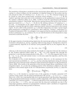
derivative parts linearly to control the system. Fig. 1 shows the block diagram of the C-PID
controller.

Proportion
Integration
Differentiation
+
+
+
-
r(t)
Controlled
object
y(t)
e(t) u(t)

Fig. 1. Block diagram of the C-PID controller

The algorithm of C-PID controller can be given as follows:








tytrte



(1)

     










dt
tde
Tdtte
T
teKtu
d
i
p
1
(2)

where y(t) is the output of the system, r(t) is the reference input of the system, e(t) is the
error signal between y(t) and r(t), u(t) is the output of the C-PID controller, K
p
is proportional
gain, T

i
is integral time constant and T
d
is derivative time constant.
Equation (2) also can be rewritten as (3):


     


dt
tde
KdtteKteKtu
dip


(3)

where K
i
is integral gain, K
d
is derivative gain, and K
i
=K
p
/T
i
, K
d

=K
p
T
d
.
In C-PID controller, the relation between PID parameters and the system response
specifications is clear. Each part has its certain function as follows (Shi & Hao, 2008):
(1) Proportion can increase the response speed and control accuracy of the system. Bigger
K
p
can lead to faster response speed and higher control accuracy. But if K
p
is too big, the
overshoot will be large and the system will tend to be instable. Meanwhile, if K
p
is too
small, the control accuracy will be decreased and the regulating time will be prolonged.
The static and dynamic performance will be deteriorated.
(2) Integration is used to eliminate the steady-state error of the system. With bigger K
i
, the
steady-state error can be eliminated faster. But if K
i
is too big, there will be integral
saturation at the beginning of the control process and the overshoot will be large. On
the other hand, if K
i
is too small, the steady-state error will be very difficult to be
eliminated and the control accuracy will be bad.
(3) Differentiation can improve the dynamic performance of the system. It can inhibit and

predict the change of the error in any direction. But if K
d
is too big, the response process
will brake early, the regulating time will be prolonged and the anti-interference
capability of the system will be bad.

The three gains of C-PID controller, K
p
, K
i
and K
d
, can be determined conveniently according
to the above mentioned function of each part. There are many methods such as NCD (Wei,
2004; Qin et al., 2005) and genetic algorithm can be used to determine the gains effectively.
(1) NCD is a toolbox in Matlab. It is developed for the design of nonlinear system
controller. On the basis of graphical interfaces, it integrates the functions of
optimization and simulation for nonlinear system controller in Simulink mode.
(2) Genetic algorithm (GA) is a stochastic optimization algorithm modeled on the
principles and concepts of natural selection and evolution. It has outstanding abilities
for solving multi-objective optimization problems and finding global optimal solutions.
GA can readily handle discontinuous and nondifferentiable functions. In addition, it is
easily programmed and conveniently implemented (Naayagi & Kamaraj, 2005;
Vasconcelos et al., 2001).
In many conventional applications, the gains of C-PID controller are determined offline by
one of the methods mentioned above and then fixed during the whole control process. This
control scheme has two obvious shortcomings as follows:
(1) All the methods that can be used to determine the gains of C-PID controller offline are
based on the precise mathematical model of the controlled system. However, in many
applications, such as motor drive system, it is very difficult to build the precise

mathematical model due to the multivariable, time-variant, strong nonlinearity and
strong coupling of the real plant.
(2) In many applications, some parameters of the controlled system are not constant. They
will be changed according to different operation conditions. For example, in motor
drive system, the winding resistance of the motor will be changed nonlinearly along
with the temperature. If the gains of C-PID controller are still fixed, the performance of
the system will deteriorate.
To overcome these disadvantages, C-PID should be improved. The gains of PID controller
should be adjusted dynamically during the control process.

3. Improved PID Controller
There are many techniques such as fuzzy logic control, neural network and expert control
(Xu et al., 2004) can be adopted to adjust the gains online according to different conditions.
In this chapter, two kinds of Improved PID (I-PID) controller based on fuzzy logic control
and neural network are studied in detail.

3.1 Fuzzy Self-tuning PID Controller
Fuzzy logic control (FLC) is a typical intelligent control method which has been widely used
in many fields, such as steelmaking, chemical industry, household appliances and social
sciences. The biggest feature of FLC is it can express empirical knowledge of the experts by
inference rules. It does not need the mathematical model of the controlled object. What’s
more, it is not sensitive to parameters changing and it has strong robustness. In summary,
FLC is very suitable for the controlled object with characteristics of large delay, large inertia,
non-linear and time-variant (Liu & Li, 2010; Liu & Song, 2006; Shi & Hao, 2008).
The structure of a SISO (single input single output) FLC is shown in Fig. 2. It can be found
that the typical FLC consists of there main parts as follows:

PID Control, Implementation and Tuning94

Fuzzification

Fuzzy Inference
Machine
Defuzzification
Crisp Vague CrispVague
x
u

Fig. 2. The structure of SISO FLC

(1) Fuzzification comprises the process of transforming crisp inputs into grades of
membership for linguistic terms of fuzzy sets. The input values of a FLC consist of
measured values from the plant that are either plant output values or plant states, or
control errors derived from the set-point values and the controlled variables.
(2) Fuzzy Inference Machine is the core of a fuzzy control system. It combines the facts
obtained from the fuzzification with the rule base and conducts the fuzzy reasoning
process. A proper rule base can be found either by asking experts or by evaluation of
measurement data using data mining methods.
(3) Defuzzification transforms an output fuzzy set back to a crisp value. Many methods
can be used for defuzzification, such as centre of gravity method (COG), centre of
singleton method (COS) and maximum methods.
Detailed analyses show that FLC is a nonlinear PD controller. It cannot eliminate steady-
state error when the controlled object does not have integral element, so it is a ragged
controller. To overcome this disadvantage, FLC is often used together with other controllers.
Fig. 3 shows the structure of a controller called Fuzzy_PID compound controller. When the
error is big, FLC is used to accelerate the dynamic response, and when the error is small,
PID controller is used to enhance the steady-state accuracy of the system (Liu & Song, 2006).

FLC
PID Controller
+

-
r(t)
Controlled
object
y(t)
e(t)
u(t)
Switch Logic
d/dt

Fig. 3. The structure of Fuzzy_PID compound controller

d/dt
FLC
C-PID
Parameters Tuning
C-PID Controller
ΔK
p
ΔK
i
ΔK
d
K
p
K
i
K
d
Initial

Parameters Set
K
p0
K
i0
K
d0
Controlled Object
r(t)
y(t)
e(t)
ec(t)
+
-

Fig. 4. The structure of FPID controller


In this chapter, an I-PID controller called fuzzy self-tuning PID (FPID) controller is
introduced. In this controller, FLC is used to tune the parameters of C-PID controller online
according to different conditions. Fig. 4 shows the structure of FPID controller (Liu & Li,
2010).
In FPID controller, the error signal and the rate of change of error are inputted into FLC
firstly. After fuzzy inference based on the rule base, the increments of PID control
parameters, ∆K
p
, ∆K
i
and ∆K
d

, are obtained, add these increments to initial values of PID
control parameters, the actual PID control parameters can be achieved finally. The initial
values of PID control parameters, K
p0
, K
i0
and K
d0
, can be obtained by the methods
mentioned in the last section.

3.2 Neural Network PID Controller
Neural network (NN) is a mathematical model or computational model inspired by the
structure and functional aspects of biological neural systems, such as the brain. It is
composed of a large number of highly interconnected processing elements (neurones)
working in unison to solve specific problems. Fig. 5 shows the typical structure of a NN. It
has one input layer, one output layer and several hidden layers. In each layer, there are a
certain number of nodes (neurons). The neurons in adjacent layers are connected together,
while there are no connections between neurons in the same layer. Just like the biological
neural systems, the NN also can learn by itself. During the learning phase, the connection
strength (weights) between neurons can be adjusted by certain algorithms automatically
based on external or internal information that flows through the network. (Tao, 2002; Liu,
2003; Wang et al., 2007)

Input layer
Hidden layers
Output layer

Fig. 5. The structure of a typical NN

The greatest advantage of NN is its ability to be used as an arbitrary function approximation
mechanism which 'learns' from observed data. There are many other remarkable advantages
of NN as follows:
(1) Adaptive learning: An ability to learn how to do tasks based on the data given for
training or initial experience.
(2) Real time operation: NN can process massive data and information in parallel. Special
hardware devices are being designed and manufactured which take advantage of this
capability.
(3) Fault tolerance: Some capabilities of NN can be retained even with major network
damage.
Application of Improved PID Controller in Motor Drive System 95

Fuzzification
Fuzzy Inference
Machine
Defuzzification
Crisp Vague CrispVague
x
u

Fig. 2. The structure of SISO FLC

(1) Fuzzification comprises the process of transforming crisp inputs into grades of
membership for linguistic terms of fuzzy sets. The input values of a FLC consist of
measured values from the plant that are either plant output values or plant states, or
control errors derived from the set-point values and the controlled variables.
(2) Fuzzy Inference Machine is the core of a fuzzy control system. It combines the facts
obtained from the fuzzification with the rule base and conducts the fuzzy reasoning
process. A proper rule base can be found either by asking experts or by evaluation of
measurement data using data mining methods.

(3) Defuzzification transforms an output fuzzy set back to a crisp value. Many methods
can be used for defuzzification, such as centre of gravity method (COG), centre of
singleton method (COS) and maximum methods.
Detailed analyses show that FLC is a nonlinear PD controller. It cannot eliminate steady-
state error when the controlled object does not have integral element, so it is a ragged
controller. To overcome this disadvantage, FLC is often used together with other controllers.
Fig. 3 shows the structure of a controller called Fuzzy_PID compound controller. When the
error is big, FLC is used to accelerate the dynamic response, and when the error is small,
PID controller is used to enhance the steady-state accuracy of the system (Liu & Song, 2006).

FLC
PID Controller
+
-
r(t)
Controlled
object
y(t)
e(t)
u(t)
Switch Logic
d/dt

Fig. 3. The structure of Fuzzy_PID compound controller

d/dt
FLC
C-PID
Parameters Tuning
C-PID Controller

ΔK
p
ΔK
i
ΔK
d
K
p
K
i
K
d
Initial
Parameters Set
K
p0
K
i0
K
d0
Controlled Object
r(t)
y(t)
e(t)
ec(t)
+
-

Fig. 4. The structure of FPID controller

In this chapter, an I-PID controller called fuzzy self-tuning PID (FPID) controller is
introduced. In this controller, FLC is used to tune the parameters of C-PID controller online
according to different conditions. Fig. 4 shows the structure of FPID controller (Liu & Li,
2010).
In FPID controller, the error signal and the rate of change of error are inputted into FLC
firstly. After fuzzy inference based on the rule base, the increments of PID control
parameters, ∆K
p
, ∆K
i
and ∆K
d
, are obtained, add these increments to initial values of PID
control parameters, the actual PID control parameters can be achieved finally. The initial
values of PID control parameters, K
p0
, K
i0
and K
d0
, can be obtained by the methods
mentioned in the last section.

3.2 Neural Network PID Controller
Neural network (NN) is a mathematical model or computational model inspired by the
structure and functional aspects of biological neural systems, such as the brain. It is
composed of a large number of highly interconnected processing elements (neurones)
working in unison to solve specific problems. Fig. 5 shows the typical structure of a NN. It
has one input layer, one output layer and several hidden layers. In each layer, there are a

certain number of nodes (neurons). The neurons in adjacent layers are connected together,
while there are no connections between neurons in the same layer. Just like the biological
neural systems, the NN also can learn by itself. During the learning phase, the connection
strength (weights) between neurons can be adjusted by certain algorithms automatically
based on external or internal information that flows through the network. (Tao, 2002; Liu,
2003; Wang et al., 2007)

Input layer
Hidden layers
Output layer

Fig. 5. The structure of a typical NN

The greatest advantage of NN is its ability to be used as an arbitrary function approximation
mechanism which 'learns' from observed data. There are many other remarkable advantages
of NN as follows:
(1) Adaptive learning: An ability to learn how to do tasks based on the data given for
training or initial experience.
(2) Real time operation: NN can process massive data and information in parallel. Special
hardware devices are being designed and manufactured which take advantage of this
capability.
(3) Fault tolerance: Some capabilities of NN can be retained even with major network
damage.
PID Control, Implementation and Tuning96

BP (backpropagation) neural network (BPNN) is the most popular neural network for
practical applications. It adopts the backpropagation learning algorithm which can be
divided into two phases: data feedforward and error backpropagation.
(1) Data feedforward: In this phase, the data, such as the error of the controlled system,
inputted into the input layer is fed into the hidden layer and then into the output layer.

Finally, the output of the BPNN can be obtained from the output layer. It is the function
of the connection weights between neurons.
(2) Error backpropagation: In this phase, the actual output value of the network obtained
in the last phase is compared with a desired value. The error between them is
propagated backward. The connection weights between neurons are adjusted by some
means, such as gradient descent algorithm, based on the error.
These two phases are repeated continuously until the performance of the network is good
enough.
In this chapter, BPNN is used to tune the parameters of C-PID controller online. Fig. 6 shows
the structure of this I-PID controller named NNPID controller.

u(t)
BPNN
C-PID controller
+
-
r(t) e(t)
Controlled
object
y(t)
K
p
K
i
K
d

Fig. 6. The structure of NNPID controller

It can be seen that NNPID controller consists of C-PID controller and BPNN. C-PID

controller is used to control the plant directly. Its output, u(t), can be obtained by (3). In
order to optimize the performance of the system, BPNN is used to adjust the three
parameters of C-PID controller online based on some state variables of the system.

4. Motor Drive System
Motor is the main controlled object in motor drive system. In practical applications, there
are many kinds of motors. In this chapter, the brushless DC motor (BLDCM) and switched
reluctance motor (SRM) are studied as examples. Their mathematical models are built to
simulate the performance of different control methods.

4.1 Brushless DC Motor
In BLDCM, electronic commutating device is used instead of the mechanical commutating
device. Because BLDCM has many remarkable advantages, such as high efficiency, silent
operation, high power density, low maintenance, high reliability and so on, it has been
widely used in many industrial and domestic applications.



The voltage equation for one phase in BLDCM can be written as:


dt
di
LRieu
a
aaa

(4)

where u, i

a
, R
a
and L
a
are the voltage, current, resistance and inductance of one phase,
respectively. e is the back EMF (electromotive force) which can be calculated by



ve
knCe 
(5)

where ω is the angular speed of the rotor, k
v
is a constant which can be calculated by



eev
CCk 9.55
30

(6)

where C
e
is the EMF constant and Ф is the flux per pole.
The torque equation can be given as

dt
d
JBTT
Lem



(7)

where T
em
is electromagnetic torque, T
L
is load torque, B is damping coefficient and J is
rotary inertia.
T
em
also can be obtained by


ataTem
ikiCT  (8)

where k
t
is a constant which can be calculated by



Tt
Ck (9)

where C
T
is the torque constant.
Based on all above equations, the state space equation of BLDCM can be obtained as


















































L
a

a
t
a
v
a
a
a
T
u
J
L
i
J
B
J
k
L
k
L
R
i
dt
d
1
0
0
1

(10)

The Laplace transform of (10) can be written as two equations as follows:


 




 
 













BJs
TsIk
s
RsL
sUsk
sI
Lat

aa
v
a


(11)
Application of Improved PID Controller in Motor Drive System 97

BP (backpropagation) neural network (BPNN) is the most popular neural network for
practical applications. It adopts the backpropagation learning algorithm which can be
divided into two phases: data feedforward and error backpropagation.
(1) Data feedforward: In this phase, the data, such as the error of the controlled system,
inputted into the input layer is fed into the hidden layer and then into the output layer.
Finally, the output of the BPNN can be obtained from the output layer. It is the function
of the connection weights between neurons.
(2) Error backpropagation: In this phase, the actual output value of the network obtained
in the last phase is compared with a desired value. The error between them is
propagated backward. The connection weights between neurons are adjusted by some
means, such as gradient descent algorithm, based on the error.
These two phases are repeated continuously until the performance of the network is good
enough.
In this chapter, BPNN is used to tune the parameters of C-PID controller online. Fig. 6 shows
the structure of this I-PID controller named NNPID controller.

u(t)
BPNN
C-PID controller
+
-
r(t) e(t)

Controlled
object
y(t)
K
p
K
i
K
d

Fig. 6. The structure of NNPID controller

It can be seen that NNPID controller consists of C-PID controller and BPNN. C-PID
controller is used to control the plant directly. Its output, u(t), can be obtained by (3). In
order to optimize the performance of the system, BPNN is used to adjust the three
parameters of C-PID controller online based on some state variables of the system.

4. Motor Drive System
Motor is the main controlled object in motor drive system. In practical applications, there
are many kinds of motors. In this chapter, the brushless DC motor (BLDCM) and switched
reluctance motor (SRM) are studied as examples. Their mathematical models are built to
simulate the performance of different control methods.

4.1 Brushless DC Motor
In BLDCM, electronic commutating device is used instead of the mechanical commutating
device. Because BLDCM has many remarkable advantages, such as high efficiency, silent
operation, high power density, low maintenance, high reliability and so on, it has been
widely used in many industrial and domestic applications.

The voltage equation for one phase in BLDCM can be written as:


dt
di
LRieu
a
aaa

(4)

where u, i
a
, R
a
and L
a
are the voltage, current, resistance and inductance of one phase,
respectively. e is the back EMF (electromotive force) which can be calculated by



ve
knCe 
(5)

where ω is the angular speed of the rotor, k
v
is a constant which can be calculated by


eev
CCk 9.55
30

(6)

where C
e
is the EMF constant and Ф is the flux per pole.
The torque equation can be given as


dt
d
JBTT
Lem



(7)

where T
em
is electromagnetic torque, T
L
is load torque, B is damping coefficient and J is
rotary inertia.

T
em
also can be obtained by


ataTem
ikiCT  (8)

where k
t
is a constant which can be calculated by



Tt
Ck (9)

where C
T
is the torque constant.
Based on all above equations, the state space equation of BLDCM can be obtained as



















































L
a
a
t
a
v
a
a
a
T
u
J
L
i
J
B
J
k
L
k

L
R
i
dt
d
1
0
0
1

(10)

The Laplace transform of (10) can be written as two equations as follows:


 




 
 














BJs
TsIk
s
RsL
sUsk
sI
Lat
aa
v
a


(11)
PID Control, Implementation and Tuning98

According to (11), the simulation model of BLDCM can be built in Matlab/simulink as
shown in Fig. 7.

1/(L
a
s+R
a
)
k
t

1/(Js+B)
k
v
U
T
L
-
+ +
-I
a
ω
Load
Speed
Control

Fig. 7. The simulation model of BLDCM

4.2 Switched Reluctance Motor
The SRM is a brushless synchronous machine with salient rotor and stator teeth. There are
concentrated phase windings in the stator, and no magnets and windings in the rotor. It has
many remarkable advantages such as simple magnetless and rugged construction, simple
control, ability of extremely high speed operation, relatively wide constant power capability,
minimal effects of temperature variations offset, low manufacturing cost and ability of
hazard-free operation. These advantages make the SRM very suitable for applications in
more/all electric aircraft (M/A EA), electric vehicle (EV) and wind power generation.
Because the nonlinear model of SRM is very complex, people generally use its quasi-linear
model to design and analyze control methods.
According to the quasi-linear model of SRM, the average torque equation can be obtained as
(12) when the phase current is flat topped (Wang, 1999).

 












minmax
1
min
1
1
2
2
2
1
2
LLL
UmN
T
off
on
off

r
sr
av




(12)

where T
av
is the average torque, m is the number of motor phase, N
r
is the number of rotor
tooth, U
s
is the power supply voltage, ω
r
is angular speed of the rotor, θ
on
is the angle of
starting the excitation, θ
off
is the angle of switching off the excitation, θ
1
is the starting angle
of the phase inductance increasing, L
max
and L
min

are the maximum and minimum value of
phase inductance, respectively.
Based on (12), the total differential equation of T
av
can be written as (He et al., 2004)


r
r
av
off
off
av
on
on
av
s
s
av
av
d
T
d
T
d
T
dU
U
T
dT



















(13)
According to the linearization theory, the differential of each variable in (13) can be replaced
by corresponding increment. If voltage PWM control is adopted, θ
on
and θ
off
are fixed. The
simplified small-signal torque equation can be obtained as


rsuav
kUkT



 (14)


The increment of the average torque also can be indicated as


Lr
r
av
TB
dt
d
JT 




(15)

where J is rotary inertia, B is damping coefficient, T
L
is load torque.
The voltage chopping can be treated as a sampling process of the controller’s output
∆U
ASR
,
and the amplification factor is K
c

. The small-signal model of power inverter can be given as

)(
1
)(
1
)(
sU
Ts
T
ksU
s
e
ksU
ASRcASR
Ts
cs






(16)

The feedback of angular speed can be treated as a small inertial element.

)1/()( sTksG
n




(17)

where K
n
is feedback coefficient and T
ω
is time constant of the measurement system.
Based on above analysis, the simplified small-signal model of SRM can be got as shown in
Fig. 8.

k
u
1/(Js+B)
k
ω
U
T
L
-
+
+
-
ω
r
-
k
c
T/(1+Ts)

Controller
k
n
/(1+T
ω
s)
Speed
Load
Control
Feedback

Fig. 8. The simulation model of SRM

5. Design of I-PID Controller
5.1 FPID Controller for SRM
Based on Fig.1, Fig. 4 and Fig. 8, the simulation model of C-PID and FPID for SRM can be
obtained as shown in Fig. 9 and Fig. 10. The internal structure of the module marked “SRM”
is the part that enclosed by dashed box in Fig. 8.
It can be found that the three parameters of the PID controller in FPID control can be
obtained by











ddd
iii
ppp
KKK
KKK
KKK
0
0
0
(18)

Application of Improved PID Controller in Motor Drive System 99

According to (11), the simulation model of BLDCM can be built in Matlab/simulink as
shown in Fig. 7.

1/(L
a
s+R
a
)
k
t
1/(Js+B)
k
v
U
T
L
-

+ +
-I
a
ω
Load
Speed
Control

Fig. 7. The simulation model of BLDCM

4.2 Switched Reluctance Motor
The SRM is a brushless synchronous machine with salient rotor and stator teeth. There are
concentrated phase windings in the stator, and no magnets and windings in the rotor. It has
many remarkable advantages such as simple magnetless and rugged construction, simple
control, ability of extremely high speed operation, relatively wide constant power capability,
minimal effects of temperature variations offset, low manufacturing cost and ability of
hazard-free operation. These advantages make the SRM very suitable for applications in
more/all electric aircraft (M/A EA), electric vehicle (EV) and wind power generation.
Because the nonlinear model of SRM is very complex, people generally use its quasi-linear
model to design and analyze control methods.
According to the quasi-linear model of SRM, the average torque equation can be obtained as
(12) when the phase current is flat topped (Wang, 1999).


 













minmax
1
min
1
1
2
2
2
1
2
LLL
UmN
T
off
on
off
r
sr
av





(12)

where T
av
is the average torque, m is the number of motor phase, N
r
is the number of rotor
tooth, U
s
is the power supply voltage, ω
r
is angular speed of the rotor, θ
on
is the angle of
starting the excitation, θ
off
is the angle of switching off the excitation, θ
1
is the starting angle
of the phase inductance increasing, L
max
and L
min
are the maximum and minimum value of
phase inductance, respectively.
Based on (12), the total differential equation of T
av
can be written as (He et al., 2004)

r
r
av
off
off
av
on
on
av
s
s
av
av
d
T
d
T
d
T
dU
U
T
dT



















(13)
According to the linearization theory, the differential of each variable in (13) can be replaced
by corresponding increment. If voltage PWM control is adopted, θ
on
and θ
off
are fixed. The
simplified small-signal torque equation can be obtained as


rsuav
kUkT








(14)


The increment of the average torque also can be indicated as


Lr
r
av
TB
dt
d
JT 




(15)

where J is rotary inertia, B is damping coefficient, T
L
is load torque.
The voltage chopping can be treated as a sampling process of the controller’s output
∆U
ASR
,
and the amplification factor is K
c
. The small-signal model of power inverter can be given as

)(
1
)(
1
)( sU
Ts
T
ksU
s
e
ksU
ASRcASR
Ts
cs






(16)

The feedback of angular speed can be treated as a small inertial element.

)1/()( sTksG
n

 (17)

where K
n
is feedback coefficient and T
ω
is time constant of the measurement system.
Based on above analysis, the simplified small-signal model of SRM can be got as shown in
Fig. 8.

k
u
1/(Js+B)
k
ω
U
T
L
-
+
+
-
ω
r
-
k
c
T/(1+Ts)
Controller
k
n
/(1+T

ω
s)
Speed
Load
Control
Feedback

Fig. 8. The simulation model of SRM

5. Design of I-PID Controller
5.1 FPID Controller for SRM
Based on Fig.1, Fig. 4 and Fig. 8, the simulation model of C-PID and FPID for SRM can be
obtained as shown in Fig. 9 and Fig. 10. The internal structure of the module marked “SRM”
is the part that enclosed by dashed box in Fig. 8.
It can be found that the three parameters of the PID controller in FPID control can be
obtained by










ddd
iii
ppp
KKK

KKK
KKK
0
0
0
(18)

PID Control, Implementation and Tuning100

Where K
p0
, K
i0
and K
d0
are the initial PID parameters obtained by NCD or GA.
∆
K
p
, ∆K
i
and
∆K
d
are provided by FLC. They are used to adjust the three parameters online. In other
words, the parameters of C-PID can be dynamically tuned by FLC according to different
operation conditions. Fig. 11 shows the structure of the FLC used in FPID controller. It has
two input variables and three output variables.

Fig. 9. The simulation model of C-PID controlled SRM system


Fig. 10. The simulation model of FPID controlled SRM system


Fig. 11. Structure of the designed FLC used in FPID controller

The most important thing for the design of FPID controller is the determination of the fuzzy
rule base. According to the functions of each PID parameter mentioned in section 2, the
principles for their adjustment can be summarized as follows (Shi & Hao, 2008):
(1) When the absolute value of the system error,│e(t)│, is relatively big: K
p
is increased to
get faster tracking speed, K
i
is reduced to avoid overshoot.
(2) When │e(t)│ is relatively small: K
p
and K
i
are increased to enhance the tracking
precision, K
d
should be proper to avoid steady-state oscillation.
(3) When │e(t)│ is medium: K
p
is reduced to avoid overshoot, K
i
is increased slightly to

enhance the steady-state precision, and K
d
should be proper to guarantee the stability of
the system.
Based on above principles and consider the change rate of the system error, ec(t), the fuzzy
rule base of the three parameters can be obtained. As an example, Table.1 shows the fuzzy
rule base for ∆K
p
.


∆
K
p
ec

e
NB NM NS ZO PS PM PB
NB NB NB NM PB PB PB ZO
NM NB NB NM PM PB ZO PS
NS NB NM NS PS ZO NM NS
ZO NB NM NS ZO NS NM NB
PS NS NM ZO PS NS NM NB
PM PS ZO PB PM NM NB NB
PB ZO PB PB PB NM NB NB
Table 1. Fuzzy rule base of ∆K
p


It can be seen that there are totally 49 fuzzy rules and they are represented by fuzzy

linguistic terms, such as if e=NB and ec=NB then ∆K
p
=NB, ∆K
i
=NB, ∆K
d
=PB.
In this chapter, all the variables are described by seven linguistic terms. They are negative
big (NB), negative middle (NM), negative small (NS), zero (ZO), positive small (PS), positive
middle (PM) and positive big (PB). The universe of input variables, e and ec, is {-3 -2 -1 0 1 2
3}. The universe of output variables, ∆K
p
, ∆K
i
and ∆K
d
, is {-0.6 -0.4 -0.2 0 0.2 0.4 0.6}.
Fig. 12 and 13 show the membership function of each variable.


Fig. 12. Membership function of e and ec

Application of Improved PID Controller in Motor Drive System 101

Where K
p0
, K
i0
and K
d0

are the initial PID parameters obtained by NCD or GA.
∆
K
p
, ∆K
i
and
∆K
d
are provided by FLC. They are used to adjust the three parameters online. In other
words, the parameters of C-PID can be dynamically tuned by FLC according to different
operation conditions. Fig. 11 shows the structure of the FLC used in FPID controller. It has
two input variables and three output variables.


Fig. 9. The simulation model of C-PID controlled SRM system


Fig. 10. The simulation model of FPID controlled SRM system


Fig. 11. Structure of the designed FLC used in FPID controller

The most important thing for the design of FPID controller is the determination of the fuzzy
rule base. According to the functions of each PID parameter mentioned in section 2, the
principles for their adjustment can be summarized as follows (Shi & Hao, 2008):
(1) When the absolute value of the system error,│e(t)│, is relatively big: K
p
is increased to
get faster tracking speed, K

i
is reduced to avoid overshoot.
(2) When │e(t)│ is relatively small: K
p
and K
i
are increased to enhance the tracking
precision, K
d
should be proper to avoid steady-state oscillation.
(3) When │e(t)│ is medium: K
p
is reduced to avoid overshoot, K
i
is increased slightly to
enhance the steady-state precision, and K
d
should be proper to guarantee the stability of
the system.
Based on above principles and consider the change rate of the system error, ec(t), the fuzzy
rule base of the three parameters can be obtained. As an example, Table.1 shows the fuzzy
rule base for ∆K
p
.


∆
K
p
ec

e
NB NM NS ZO PS PM PB
NB NB NB NM PB PB PB ZO
NM NB NB NM PM PB ZO PS
NS NB NM NS PS ZO NM NS
ZO NB NM NS ZO NS NM NB
PS NS NM ZO PS NS NM NB
PM PS ZO PB PM NM NB NB
PB ZO PB PB PB NM NB NB
Table 1. Fuzzy rule base of ∆K
p


It can be seen that there are totally 49 fuzzy rules and they are represented by fuzzy
linguistic terms, such as if e=NB and ec=NB then ∆K
p
=NB, ∆K
i
=NB, ∆K
d
=PB.
In this chapter, all the variables are described by seven linguistic terms. They are negative
big (NB), negative middle (NM), negative small (NS), zero (ZO), positive small (PS), positive
middle (PM) and positive big (PB). The universe of input variables, e and ec, is {-3 -2 -1 0 1 2
3}. The universe of output variables, ∆K
p
, ∆K
i
and ∆K

d
, is {-0.6 -0.4 -0.2 0 0.2 0.4 0.6}.
Fig. 12 and 13 show the membership function of each variable.


Fig. 12. Membership function of e and ec

PID Control, Implementation and Tuning102


Fig. 13. Membership function of ∆K
p
, ∆K
i
and ∆K
d


In this chapter, the MAX-MIN method is used for fuzzy inference and centroid is used for
defuzzification.

5.2 NNPID Controller for BLDCM
Based on Fig.1 and Fig. 7, the simulation model of C-PID for BLDCM can be obtained as
shown in Fig. 14. The internal structure of the module marked “BLDCM” is the part that
enclosed by dashed box in Fig. 7.


Fig. 14. The simulation model of C-PID controlled BLDCM system

Based on Fig.5 and Fig. 6, the structure of the BPNN used in the NNPID controller is shown

in Fig.15.

r(k)
y(k)
e(k)
Input layer
Hidden layer
Output layer
Kp
Ki
Kd

Fig. 15. The structure of the BPNN used in NNPID controller

It can be seen that the adopted BPNN has three layers: one input layer, one hidden layer and
one output layer. There are three input variables and three output variables. r(k) is the

reference input of the system, y(k) is the real output of the system and e(k) is the error
between them. K
p
, K
i
and K
d
are the three parameters of the C-PID controller. There are five
nodes (neurones) in the hidden layer.
During operation, the connection strength (weights) between neurons can be adjusted
automatically through learning based on the input information. The three output variables
of NN, K
p

, K
i
and K
d
, will be changed along with the adjustment of the connection weights.
Finally, the performance of the system can be improved.
The output of nodes in input layer equals to their input. The input and output of nodes in
hidden layer and output layer can be represented as (Liu, 2003)


 
 
   
 
 
 
 
 
 
5,4,3,2,1
22
3
1
122













i
kinfkout
koutwkin
Hidden
ii
j
jiji
(19)

 
 
   
 
 
 
 
 
 
3,2,1 utput
33
5
1
133













l
kingkout
koutwkin
O
ll
i
i
lil
(20)

where
 
2
ij
w is connection weight between input and hidden layer,


3
li

w is connection weight
between hidden and output layer, f[·] and g[·] are activation functions. In this chapter, the
activation function of hidden layer is sigmoid function. Because the output variables of NN,
K
p
, K
i
and K
d
, can’t be negative, the activation function of output layer is nonnegative
sigmoid function, that is


 
  


















xx
x
xx
xx
ee
ex
xg
ee
ee
xxf
2
tanh1
][
tanh][
(21)

In this chapter, the output variables of NN are the three parameters of C-PID controller, that is






 
 
 
 











d
i
p
Kkout
Kkout
Kkout
3
3
3
2
3
1
(22)

With (19) ~ (22), NN completes the feedforward of the information. The output of the C-PID
controller can be got easily based on the three updated parameters, and then the output of
the system, y(k), can be obtained. The next step is the backpropagation of the error.
To minimize the error between y(k) and r(k), a performance index function is introduced as

Application of Improved PID Controller in Motor Drive System 103

Fig. 13. Membership function of ∆K
p
, ∆K
i
and ∆K
d


In this chapter, the MAX-MIN method is used for fuzzy inference and centroid is used for
defuzzification.

5.2 NNPID Controller for BLDCM
Based on Fig.1 and Fig. 7, the simulation model of C-PID for BLDCM can be obtained as
shown in Fig. 14. The internal structure of the module marked “BLDCM” is the part that
enclosed by dashed box in Fig. 7.


Fig. 14. The simulation model of C-PID controlled BLDCM system

Based on Fig.5 and Fig. 6, the structure of the BPNN used in the NNPID controller is shown
in Fig.15.

r(k)
y(k)
e(k)
Input layer
Hidden layer
Output layer
Kp

Ki
Kd

Fig. 15. The structure of the BPNN used in NNPID controller

It can be seen that the adopted BPNN has three layers: one input layer, one hidden layer and
one output layer. There are three input variables and three output variables. r(k) is the

reference input of the system, y(k) is the real output of the system and e(k) is the error
between them. K
p
, K
i
and K
d
are the three parameters of the C-PID controller. There are five
nodes (neurones) in the hidden layer.
During operation, the connection strength (weights) between neurons can be adjusted
automatically through learning based on the input information. The three output variables
of NN, K
p
, K
i
and K
d
, will be changed along with the adjustment of the connection weights.
Finally, the performance of the system can be improved.
The output of nodes in input layer equals to their input. The input and output of nodes in
hidden layer and output layer can be represented as (Liu, 2003)

 
 
   
 
 
 
 
 
 
5,4,3,2,1
22
3
1
122












i
kinfkout
koutwkin

Hidden
ii
j
jiji
(19)

 
 
   
 
 
 
 
 
 
3,2,1 utput
33
5
1
133













l
kingkout
koutwkin
O
ll
i
i
lil
(20)

where
 
2
ij
w is connection weight between input and hidden layer,


3
li
w is connection weight
between hidden and output layer, f[·] and g[·] are activation functions. In this chapter, the
activation function of hidden layer is sigmoid function. Because the output variables of NN,
K
p
, K
i
and K
d

, can’t be negative, the activation function of output layer is nonnegative
sigmoid function, that is


 
  

















xx
x
xx
xx
ee
ex
xg

ee
ee
xxf
2
tanh1
][
tanh][
(21)

In this chapter, the output variables of NN are the three parameters of C-PID controller, that is


 
 
 
 
 
 










d
i

p
Kkout
Kkout
Kkout
3
3
3
2
3
1
(22)

With (19) ~ (22), NN completes the feedforward of the information. The output of the C-PID
controller can be got easily based on the three updated parameters, and then the output of
the system, y(k), can be obtained. The next step is the backpropagation of the error.
To minimize the error between y(k) and r(k), a performance index function is introduced as

PID Control, Implementation and Tuning104


        
22
2
1
2
1
kekykrkJ 
(23)

Typically, the connection weights are adjusted by steepest descent method. To increase the

convergence speed, an inertia term is added.


 
 


 
 
 
1
3
3
3



 kw
w
kJ
kw
li
li
li

(24)

where η is learning rate, is inertia coefficient. In this chapter, η=0.001 and α=0.05.
Based on (19) ~ (24), the connection weights can be tuned dynamically. In this chapter, the
NNPID controller for BLDCM is implemented by M-File in Matlab.

6. Performance Verification
6.1 FPID Controller for SRM
In this chapter, the parameter values of the SRM (see Fig. 8) are as follows:
k
c
=45, T=0.5ms, k
u
=22.45, J=1kg·m
2
, B=1, k
n
=1, T
ω
=1.5ms, k
ω
=0.05.
The initial values of the three parameters in C-PID are
K
p
=5, K
i
=7, K
d
=2.
Fig. 16 shows the step response of the SRM with C-PID and FPID controller, respectively.
The reference angular speed is 100rad/s. The motor is started without load, and at 10s a
50Nm load is added.

0 5 10 15 20

0
20
40
60
80
100
120
Time (s)
Angular speed (rad/s)


FPID
C-PID

Fig. 16. The step response of the SRM

It can be seen that compared with C-PID controller, the FPID controller can improve the
performance of the system significantly. It has advantages of no overshoot, shorter adjusting
time. Moreover, when add load torque suddenly at 10s, the drop of the angular speed is
smaller and the transition time is shorter.


Fig. 17 shows the adjustment of the three parameters, K
p
, K
i
and K
d
, in FPID controller.

0 5 10 15 20
-15
-10
-5
0
5
10
15
20
25
Time (s)
K
p
, K
i
, K
d


K
p
K
i
K
d

Fig. 17. The adjustment of K
p
, K
i

and K
d
in FPID controller

It can be found that during the adjustment process of the angular speed, the three
parameters are tuned dynamically as well. When the system reaches its steady-state, the
angular speed is constant and the three parameters are also changed into their initial values.

6.2 NNPID Controller for BLDCM
The discrete form of the BLDCM used in this chapter is


u(k-1).y(k-2).y(k-1).y(k)






058310204170 (25)

where u is the output of the C-PID controller.

0 1 2 3 4 5
0
2
4
6
8
10

12
14
Time(s)
Angular speed (rad/s)


NNPID
C-PID

Fig. 18. The step response of the BLDCM

Application of Improved PID Controller in Motor Drive System 105


        
22
2
1
2
1
kekykrkJ 
(23)

Typically, the connection weights are adjusted by steepest descent method. To increase the
convergence speed, an inertia term is added.


 
 



 
 
 
1
3
3
3



 kw
w
kJ
kw
li
li
li

(24)

where η is learning rate, is inertia coefficient. In this chapter, η=0.001 and α=0.05.
Based on (19) ~ (24), the connection weights can be tuned dynamically. In this chapter, the
NNPID controller for BLDCM is implemented by M-File in Matlab.

6. Performance Verification
6.1 FPID Controller for SRM
In this chapter, the parameter values of the SRM (see Fig. 8) are as follows:
k
c

=45, T=0.5ms, k
u
=22.45, J=1kg·m
2
, B=1, k
n
=1, T
ω
=1.5ms, k
ω
=0.05.
The initial values of the three parameters in C-PID are
K
p
=5, K
i
=7, K
d
=2.
Fig. 16 shows the step response of the SRM with C-PID and FPID controller, respectively.
The reference angular speed is 100rad/s. The motor is started without load, and at 10s a
50Nm load is added.

0 5 10 15 20
0
20
40
60
80
100

120
Time (s)
Angular speed (rad/s)


FPID
C-PID

Fig. 16. The step response of the SRM

It can be seen that compared with C-PID controller, the FPID controller can improve the
performance of the system significantly. It has advantages of no overshoot, shorter adjusting
time. Moreover, when add load torque suddenly at 10s, the drop of the angular speed is
smaller and the transition time is shorter.


Fig. 17 shows the adjustment of the three parameters, K
p
, K
i
and K
d
, in FPID controller.

0 5 10 15 20
-15
-10
-5
0
5

10
15
20
25
Time (s)
K
p
, K
i
, K
d


K
p
K
i
K
d

Fig. 17. The adjustment of K
p
, K
i
and K
d
in FPID controller

It can be found that during the adjustment process of the angular speed, the three
parameters are tuned dynamically as well. When the system reaches its steady-state, the

angular speed is constant and the three parameters are also changed into their initial values.

6.2 NNPID Controller for BLDCM
The discrete form of the BLDCM used in this chapter is


u(k-1).y(k-2).y(k-1).y(k)  058310204170 (25)

where u is the output of the C-PID controller.

0 1 2 3 4 5
0
2
4
6
8
10
12
14
Time(s)
Angular speed (rad/s)


NNPID
C-PID

Fig. 18. The step response of the BLDCM

PID Control, Implementation and Tuning106

0 1 2 3 4 5
0
0.05
0.1
0.15
0.2
0.25
Time(s)
k
p
, k
i
, k
d


k
p
k
i
k
d

Fig. 19. The adjustment of K
p
, K
i
and K
d
in NNPID controller

Fig. 18 shows the step response of the BLDCM with C-PID and NNPID controller,
respectively. The reference angular speed is 10rad/s. The motor is started without load.
It can be seen that compared with C-PID controller, the NNPID controller can improve the
performance of the system significantly. The overshoot of the system is nearly eliminated.
However, because NNPID controller needs time to train NN, the adjusting times of the
system with two controllers are almost the same.
Fig. 19 shows the adjustment of the three parameters, K
p
, K
i
and K
d
, in NNPID controller.
It can be found that during the adjustment process of the angular speed, the three
parameters are tuned dynamically. When the system reaches its steady-state, the angular
speed is constant and the three parameters are constant as well.

7. Conclusion
In this chapter, the structure and operation principle of C-PID controller are introduced
firstly. According to the shortcomings of C-PID controller, two improved PID controllers,
namely FPID and NNPID controller, are studied. The structure and operation principle of
them are analyzed. Then, the BLDCM and SRM drive system are introduced and their
mathematical models are built. Based on the models, FPID and NNPID controller are
designed in detail. Finally, the performances of the designed controllers are tested by
simulation. The simulation results show that compared with C-PID controller, both FPID
and NNPID controller can improve the performance of the system significantly.

8. References
Ang K. H.; Chong G. & Li Y. (2005). PID Control System Analysis, Design, and Technology.

IEEE Transactions on Control Systems Technology, Vol.13, No.4, July 2005, 559-576,
ISSN 1063-6536.
Li X.; Mao X. & Lin W. (2010). Permanent Magnet Synchronous Motor Decoupling Control
Study Based on the Inverse System, Proceedings of Progress In Electromagnetics
Research Symposium, pp. 300-303, ISBN 978-1-934142-14-1, Cambridge, July 2010,
Electromagnetics Academy, Cambridge.

Tang K. S.; Man K. F.; Chen G. & Kwong S. (2001). An Optimal Fuzzy PID Controller. IEEE
Transactions on Industrial Electronics, Vol.48, No.4, August 2001, 757-765, ISSN 0278-
0046.
Yu H.; Zhang X. & Hu Q. (2009). Application of NN-PID Control in Linear Elevator,
Proceedings of Fifth International Conference on Natural Computation, pp. 35-37, ISBN
978-0-7695-3736-8, Tianjian, August 2009, IEEE Computer Society, Los Alamitos.
Lin C.; Jan H. & Shieh N. (2003). GA-Based Multiobjective PID Control for a Linear
Brushless DC Motor. IEEE/ASME Transactions on Mechatronics, Vol.8, No.1, March
2003, 56-65, ISSN 1083-4435.
Chen H. & Gu J. J. (2010). Implementation of the Three-Phase Switched Reluctance Machine
System for Motors and Generators. IEEE/ASME Transactions on Mechatronics,
Vol.15, No.3, June 2010, 421-432, ISSN 1083-4435.
Wu H.; Cheng S. & Cui S. (2005). A Controller of Brushless DC Motor for Electric Vehicle.
IEEE Transactions on Magnetics, Vol.41, No.1, January 2005, 509-513, ISSN 0018-9464.
Shi X. & Hao Z. (2008). Fuzzy Control and Its Simulation in Matlab, Tsinghua University Press,
ISBN 978-7-81123-029-1, Beijing.
Wei W. (2004). MATLAB control engineering toolbox technique manual, National Defence
Industrial Press, ISBN 7-118-03205-0, Beijing.
Qin G.; Yao W. & Zhang W. (2005). Design of Nonlinear Optimization PID Controller for
BLDCM Based on Neuro-Fuzzy Identified Model, Proceedings of the Eighth
International Conference on Electrical Machines and Systems, pp. 1524-1527, ISBN 7-
5062-7407-8, Nanjing, September 2005, Beijing World Publishing Corporation,
Beijing.

Naayagi R. T. & Kamaraj V. (2005). Shape Optimization of Switched Reluctance Machine for
Aerospace Applications, Proceedings of 31st Annual Conference of IEEE Industrial
Electronics Society, pp. 1748-1751, ISBN 0-7803-9252-3, Raleigh, November 2005,
IEEE Industrial Electronics Society, Los Alamitos.
Vasconcelos J. A.; Ramirez J. A.; Takahashi R. H. C. & Saldanha R. R. (2001). Improvements
in Genetic Algorithms. IEEE Transactions on Magnetics, Vol.37, No.5, September
2001, 3414-3417, ISSN 0018-9464.
Xu J.; Zhao J.; Luo L. & Wan S. (2004). Expert PID Control for AC/DC Converter, Proceedings
of The Fifth World Congress on Intelligent Control and Automation, pp. 5586-5590, ISBN
0-7803-8273-0, Hangzhou, June 2004, IEEE Industrial Electronics Chapter,
Singapore.
Liu X. & Li X. (2010). Research on Tension Control System Based on Fuzzy Self-tuning PID
Control, Proceedings of 2010 Chinese Control and Decision Conference, pp. 3385-3390,
ISBN 978-1-4244-5182-1, Xuzhou, May 2010, IEEE Industrial Electronics Chapter,
Singapore.
Liu W. & Song S. (2006). Application of Fuzzy Control in Switched Reluctance Motor Speed
Regulating System, Proceedings of International Conference on Computational
Intelligence for Modelling, Control and Automation, pp. 72-72, ISBN 0-7695-2731-0,
Sydney, November 2006, Patrick Kellenberger, Sydney.
Tao Y. (2002). Novel PID Control and Its Application, China Machine Press, ISBN 7-111-06299-
X, Beijing.
Liu J. (2003). Novel PID Control and Its Simulation in Matlab, Publishing House of Electronic
Industry, ISBN 7-5053-8427-9, Beijing.
Application of Improved PID Controller in Motor Drive System 107

0 1 2 3 4 5
0
0.05
0.1
0.15

0.2
0.25
Time(s)
k
p
, k
i
, k
d


k
p
k
i
k
d

Fig. 19. The adjustment of K
p
, K
i
and K
d
in NNPID controller

Fig. 18 shows the step response of the BLDCM with C-PID and NNPID controller,
respectively. The reference angular speed is 10rad/s. The motor is started without load.
It can be seen that compared with C-PID controller, the NNPID controller can improve the
performance of the system significantly. The overshoot of the system is nearly eliminated.

However, because NNPID controller needs time to train NN, the adjusting times of the
system with two controllers are almost the same.
Fig. 19 shows the adjustment of the three parameters, K
p
, K
i
and K
d
, in NNPID controller.
It can be found that during the adjustment process of the angular speed, the three
parameters are tuned dynamically. When the system reaches its steady-state, the angular
speed is constant and the three parameters are constant as well.

7. Conclusion
In this chapter, the structure and operation principle of C-PID controller are introduced
firstly. According to the shortcomings of C-PID controller, two improved PID controllers,
namely FPID and NNPID controller, are studied. The structure and operation principle of
them are analyzed. Then, the BLDCM and SRM drive system are introduced and their
mathematical models are built. Based on the models, FPID and NNPID controller are
designed in detail. Finally, the performances of the designed controllers are tested by
simulation. The simulation results show that compared with C-PID controller, both FPID
and NNPID controller can improve the performance of the system significantly.

8. References
Ang K. H.; Chong G. & Li Y. (2005). PID Control System Analysis, Design, and Technology.
IEEE Transactions on Control Systems Technology, Vol.13, No.4, July 2005, 559-576,
ISSN 1063-6536.
Li X.; Mao X. & Lin W. (2010). Permanent Magnet Synchronous Motor Decoupling Control
Study Based on the Inverse System, Proceedings of Progress In Electromagnetics
Research Symposium, pp. 300-303, ISBN 978-1-934142-14-1, Cambridge, July 2010,

Electromagnetics Academy, Cambridge.

Tang K. S.; Man K. F.; Chen G. & Kwong S. (2001). An Optimal Fuzzy PID Controller. IEEE
Transactions on Industrial Electronics, Vol.48, No.4, August 2001, 757-765, ISSN 0278-
0046.
Yu H.; Zhang X. & Hu Q. (2009). Application of NN-PID Control in Linear Elevator,
Proceedings of Fifth International Conference on Natural Computation, pp. 35-37, ISBN
978-0-7695-3736-8, Tianjian, August 2009, IEEE Computer Society, Los Alamitos.
Lin C.; Jan H. & Shieh N. (2003). GA-Based Multiobjective PID Control for a Linear
Brushless DC Motor. IEEE/ASME Transactions on Mechatronics, Vol.8, No.1, March
2003, 56-65, ISSN 1083-4435.
Chen H. & Gu J. J. (2010). Implementation of the Three-Phase Switched Reluctance Machine
System for Motors and Generators. IEEE/ASME Transactions on Mechatronics,
Vol.15, No.3, June 2010, 421-432, ISSN 1083-4435.
Wu H.; Cheng S. & Cui S. (2005). A Controller of Brushless DC Motor for Electric Vehicle.
IEEE Transactions on Magnetics, Vol.41, No.1, January 2005, 509-513, ISSN 0018-9464.
Shi X. & Hao Z. (2008). Fuzzy Control and Its Simulation in Matlab, Tsinghua University Press,
ISBN 978-7-81123-029-1, Beijing.
Wei W. (2004). MATLAB control engineering toolbox technique manual, National Defence
Industrial Press, ISBN 7-118-03205-0, Beijing.
Qin G.; Yao W. & Zhang W. (2005). Design of Nonlinear Optimization PID Controller for
BLDCM Based on Neuro-Fuzzy Identified Model, Proceedings of the Eighth
International Conference on Electrical Machines and Systems, pp. 1524-1527, ISBN 7-
5062-7407-8, Nanjing, September 2005, Beijing World Publishing Corporation,
Beijing.
Naayagi R. T. & Kamaraj V. (2005). Shape Optimization of Switched Reluctance Machine for
Aerospace Applications, Proceedings of 31st Annual Conference of IEEE Industrial
Electronics Society, pp. 1748-1751, ISBN 0-7803-9252-3, Raleigh, November 2005,
IEEE Industrial Electronics Society, Los Alamitos.
Vasconcelos J. A.; Ramirez J. A.; Takahashi R. H. C. & Saldanha R. R. (2001). Improvements

in Genetic Algorithms. IEEE Transactions on Magnetics, Vol.37, No.5, September
2001, 3414-3417, ISSN 0018-9464.
Xu J.; Zhao J.; Luo L. & Wan S. (2004). Expert PID Control for AC/DC Converter, Proceedings
of The Fifth World Congress on Intelligent Control and Automation, pp. 5586-5590, ISBN
0-7803-8273-0, Hangzhou, June 2004, IEEE Industrial Electronics Chapter,
Singapore.
Liu X. & Li X. (2010). Research on Tension Control System Based on Fuzzy Self-tuning PID
Control, Proceedings of 2010 Chinese Control and Decision Conference, pp. 3385-3390,
ISBN 978-1-4244-5182-1, Xuzhou, May 2010, IEEE Industrial Electronics Chapter,
Singapore.
Liu W. & Song S. (2006). Application of Fuzzy Control in Switched Reluctance Motor Speed
Regulating System, Proceedings of International Conference on Computational
Intelligence for Modelling, Control and Automation, pp. 72-72, ISBN 0-7695-2731-0,
Sydney, November 2006, Patrick Kellenberger, Sydney.
Tao Y. (2002). Novel PID Control and Its Application, China Machine Press, ISBN 7-111-06299-
X, Beijing.
Liu J. (2003). Novel PID Control and Its Simulation in Matlab, Publishing House of Electronic
Industry, ISBN 7-5053-8427-9, Beijing.
PID Control, Implementation and Tuning108

Wang J.; Zhang C.; Jing Y. & An D. (2007). Study of Neural Network PID Control in
Variable-frequency Air-conditioning System, Proceedings of IEEE International
Conference on Control and Automation, pp. 317-322, ISBN 1-4244-0818-0, Guangzhou,
May 2007, IEEE Control Systems Chapter, Singapore.
Wang H. (1999). Switched Reluctance Motor Speed Adjusting System, China Machine Press,
ISBN 7111-04623-4, Beijing.
He L.; Wan P. & Xiao H. (2004). Application of PID-Fuzzy Controller in Switched Reluctance
Motor Drives. Middle and Small Motor, Vol.31, No.4, August 2004, 32-35, ISSN 1001-
8085.
PID control with gravity compensation for hydraulic 6-DOF parallel manipulator 109

PID control with gravity compensation for hydraulic 6-DOF parallel
manipulator
Chifu Yang, Junwei Han, O.Ogbobe Peter and Qitao Huang

*
Correspondence to: C.F Yang, State Key Laboratory of Robotics and System, Harbin
Institute of Technology, Harbin, Heilongjiang, 150001, China.
E-mail: ; Tel: +86-451-86412548(325); Fax: +86-451-86412258

Contract/grant sponsor: China Academy of Space Technology;
contract/grant number: HgdJG00401D04
Contract/grant sponsor:
State Key Laboratory of Robotics and System (HIT);
contract/grant number: SKLRS200803B





X

PID control with gravity compensation for
hydraulic 6-DOF parallel manipulator

Chifu Yang
*
, Junwei Han
O.Ogbobe Peter, and Qitao Huang

State Key Laboratory of Robotics and System,, Harbin Institute of Technology,

Harbin, Heilongjiang, 150001, China

Abstract
A novel model-based controller for 6 degree-of-freedom (DOF) hydraulic driven parallel
manipulator considering the nonlinear characteristic of hydraulic systems-proportional plus
derivative with dynamic gravity compensation controller is presented, in order to improve
control performance and eliminate steady state errors. In this paper, 6-DOF parallel
manipulator is described as multi-rigid-body systems, the dynamic models including
mechanical system and hydraulic driven system are built using Kane method and
hydromechanics methodology, the numerical forward kinematics and inverse kinematics is
solved with Newton-Raphson method and close-form solutions. The model-based controller
is developed with feedback of actuator length, desired trajectories and system states
acquired by forward kinematics solution as the input and servovalve current as its output.
The hydraulic system is decoupled by local velocity compensation in inner control loop
prerequisite for the controller. The performance revolving stability, accuracy and robustness
of the proposed control scheme for 6-DOF parallel manipulator is analyzed in theory and
simulation. The theoretical analysis and simulation results indicate the controller can
improve the control performance and eliminate the steady state errors of 6-DOF hydraulic
driven parallel manipulator.
Keywords: Parallel manipulator; Proportional-derivative control; Hydraulic servo-systems;
Dynamic compensation

5
PID Control, Implementation and Tuning110

1. Introduction
Hydraulic driven 6-DOF parallel manipulator with long stroke actuators and heavy load is
applied in most of the current high fidelity simulators, which is used to simulate various
motions in different environments by exporting varying position and orientation. There are
several advantages in the application of hydraulic driven parallel manipulator which

includes large output force and torque, higher rigidity and accuracy due to the parallel path
and averaged link to end effectors error, compared with serial manipulator [1-2]. A classical
proportional plus integral plus derivative controller is applied in hydraulic driven 6-DOF
parallel manipulator continually due to easy to implementation [3], nevertheless the
existence of large steady state errors and dynamic errors in virtue of the influence of system
gravity taken no account of hydraulic and mechanical systems in classical proportional plus
integral plus derivative control system may degrade the control performance. Well-known
facts, it is very difficult for the classical PID control to satisfy the requirements, less steady
state error and superior dynamic performance simultaneously. With respect to hydraulic 6-
DOF parallel manipulator with heavy payload, the system gravity, the uppermost
turbulence to control system for slow motion, results in large steady and dynamic errors in
gravitational direction. Therefore, the design and realization of proportional plus derivative
controller with dynamic gravity compensation in hydraulic 6-DOF parallel manipulator is of
critical importance for improving system control performance of hydraulic driven 6-DOF
parallel manipulator especially for the parallel manipulator with heavy payload.
Parallel manipulator has been extensively studied due to its high force-to-weight ratio and
widespread application [4]. 6-DOF parallel manipulator is named Stewart platform after
Stewart illustrated the use of such parallel structure [5], it is also referred to as Gough-
platform who presented the practical use of such a system [6]. Hunt [7] researched the
kinematics of parallel manipulators based on screw theory and enumerated promising
kinematics structures. Do and Yang [8] used the Newton-Euler approach to solve the
inverse dynamics for Stewart platform assuming the joints as frictionless and legs
asymmetrical. The control strategies for parallel manipulator may be largely divided into
two schemes, joint-space control developed in joint space coordinates [9-11], and workspace
control designed based on the workspace coordinates [12-14]. The joint space control
scheme can be readily implemented as a collection of multiple, independent single-input
single-output control system using data on each actuator length only. A classical
proportional plus integral plus derivative control in joint space has been employed in
industry, but it does not always guarantee a high performance for parallel robots [15]. This
novel joint space control approaches have been proposed to improve control performance

by rejecting the uncertainty and nonlinear effects in motion equations. Kim proposed a
robust nonlinear control scheme in joint space for a hydraulic parallel system based on
Lyapunov redesign method [10], yet the pressure closed loop control is hard to
implemented for real hydraulic system due to the effect of pipeline pressure transient and
frication force. Nguyen et al [11] developed a joint-space adaptive control scheme applied to
an electromechanically driven Stewart platform using Lyapunov direct method. Su
presented a robust auto-disturbance rejection controller in joint space for 6-DOF parallel
manipulator [16]. Kim et al [12] discussed robust nonlinear task space control with a friction
estimator for dynamoelectric Gough-Stewart platform. Burdet et al [17] investigated a
nonlinear controller with dynamic compensation which depended on system state and
velocity of 6-DOF parallel manipulator. Noriega et al [18] presented a neural network

control scheme and showed its superiority over a kinematics control. Kim et al [19]
researched and applied a high speed tracking control for 6-DOF electric driven Stewart
platform using an enhanced sliding mode control approach. Cervantes et al [20] studied
tracking problem of robot manipulator based on multi-rigid body models with revolute
joints via PID control. Although the above advanced model-based control strategies are
effective for 6-DOF parallel manipulator, the characteristics of hydraulic driven system is
not taken into account. Davliakos et al [21] developed operational error joint feedback
control scheme embedding the forward kinematics in the feedback control loop for 6-DOF
electrohydraulic Parallel manipulator platforms. However, only simulation is investigated
for the model-based control scheme. Besides, the influences of dynamical gravity to system
control performance are not analyzed and attracted attention for the proposed controller.
In this paper, a proportional plus derivative controller with dynamic gravity compensation
(PDGC) is developed to improve the control performance including steady and dynamic
precision via compensating steady state errors and reducing dynamic errors for a 6-DOF
hydraulic driven parallel manipulator with symmetric joint locations. This paper begins
with a practical strategy to obtain 6-DOF hydraulic driven Gough-Stewart platform essential
to the developed controller. The dynamics models of the 6-DOF platform system are built
using Kane method, considering the Gough-Stewart platform as 13 rigid bodies, and the

hydraulic driven system are established in terms of hydromechanics theory. The desired
actuator length is calculated by a closed-solution inverse kinematics, and the system states
of 6-DOF Gough-Stewart platform are obtained by a numerical forward kinematics, the
forward kinematics and inverse kinematics models are described with Newton-Raphson
method and closed-form solution, respectively. The proportional plus derivative with
dynamics compensation control scheme is gained, combing the kinematics control and
inverse dynamics method, the proposed controller employs rigid body and actuation
dynamic and yields the input current vector of the servovalve, the dynamic gravity term
including the gravity of platform, load and hydraulic cylinders is used to compensate the
influence of gravity of 6-DOF Gough-Stewart platform, and the decoupling of hydraulic
system is implemented by local velocity compensation in inner control loop. The
performance including stability, precision and robustness of the proposed controller is
analyzed in theory and simulation. The proportional plus derivative with dynamic
compensation control scheme is studied to improve the performance of control system for 6-
DOF hydraulic driven Gough-Stewart platform.

2. System model
The kinematics of 6-DOF Gough-Stewart platform has been studied extensively [22, 23].
Therefore, the kinematics models of 6-DOF Gough-Stewart are briefly described in the
paper. Fig.1 depicts the configuration of the 6-DOF Gough-Stewart; Fig.2 explains the two
Cartesian coordinate systems; the {B} coordinate system is the body coordinate system fixed
to the movement platform, while the {L} coordinate system is the base coordinate system for
the inertial frame. The linear motions denotes as surge (q
1
), sway (q
2
), and heave (q
3
) are
along the X

L
-Y
L
-Z
L
axis for base coordinate system, and the angular motions labeled as roll
(q
4
), pitch (q
5
), and yaw (q
6
) are Euler angles of platform at X
L
, Y
L
, Z
L
axis. The body
coordinate system {B} and the base coordinate system {L} are superposition in the initial
state q
i
=0, i=1,…,6.
PID control with gravity compensation for hydraulic 6-DOF parallel manipulator 111

1. Introduction
Hydraulic driven 6-DOF parallel manipulator with long stroke actuators and heavy load is
applied in most of the current high fidelity simulators, which is used to simulate various
motions in different environments by exporting varying position and orientation. There are
several advantages in the application of hydraulic driven parallel manipulator which

includes large output force and torque, higher rigidity and accuracy due to the parallel path
and averaged link to end effectors error, compared with serial manipulator [1-2]. A classical
proportional plus integral plus derivative controller is applied in hydraulic driven 6-DOF
parallel manipulator continually due to easy to implementation [3], nevertheless the
existence of large steady state errors and dynamic errors in virtue of the influence of system
gravity taken no account of hydraulic and mechanical systems in classical proportional plus
integral plus derivative control system may degrade the control performance. Well-known
facts, it is very difficult for the classical PID control to satisfy the requirements, less steady
state error and superior dynamic performance simultaneously. With respect to hydraulic 6-
DOF parallel manipulator with heavy payload, the system gravity, the uppermost
turbulence to control system for slow motion, results in large steady and dynamic errors in
gravitational direction. Therefore, the design and realization of proportional plus derivative
controller with dynamic gravity compensation in hydraulic 6-DOF parallel manipulator is of
critical importance for improving system control performance of hydraulic driven 6-DOF
parallel manipulator especially for the parallel manipulator with heavy payload.
Parallel manipulator has been extensively studied due to its high force-to-weight ratio and
widespread application [4]. 6-DOF parallel manipulator is named Stewart platform after
Stewart illustrated the use of such parallel structure [5], it is also referred to as Gough-
platform who presented the practical use of such a system [6]. Hunt [7] researched the
kinematics of parallel manipulators based on screw theory and enumerated promising
kinematics structures. Do and Yang [8] used the Newton-Euler approach to solve the
inverse dynamics for Stewart platform assuming the joints as frictionless and legs
asymmetrical. The control strategies for parallel manipulator may be largely divided into
two schemes, joint-space control developed in joint space coordinates [9-11], and workspace
control designed based on the workspace coordinates [12-14]. The joint space control
scheme can be readily implemented as a collection of multiple, independent single-input
single-output control system using data on each actuator length only. A classical
proportional plus integral plus derivative control in joint space has been employed in
industry, but it does not always guarantee a high performance for parallel robots [15]. This
novel joint space control approaches have been proposed to improve control performance

by rejecting the uncertainty and nonlinear effects in motion equations. Kim proposed a
robust nonlinear control scheme in joint space for a hydraulic parallel system based on
Lyapunov redesign method [10], yet the pressure closed loop control is hard to
implemented for real hydraulic system due to the effect of pipeline pressure transient and
frication force. Nguyen et al [11] developed a joint-space adaptive control scheme applied to
an electromechanically driven Stewart platform using Lyapunov direct method. Su
presented a robust auto-disturbance rejection controller in joint space for 6-DOF parallel
manipulator [16]. Kim et al [12] discussed robust nonlinear task space control with a friction
estimator for dynamoelectric Gough-Stewart platform. Burdet et al [17] investigated a
nonlinear controller with dynamic compensation which depended on system state and
velocity of 6-DOF parallel manipulator. Noriega et al [18] presented a neural network

control scheme and showed its superiority over a kinematics control. Kim et al [19]
researched and applied a high speed tracking control for 6-DOF electric driven Stewart
platform using an enhanced sliding mode control approach. Cervantes et al [20] studied
tracking problem of robot manipulator based on multi-rigid body models with revolute
joints via PID control. Although the above advanced model-based control strategies are
effective for 6-DOF parallel manipulator, the characteristics of hydraulic driven system is
not taken into account. Davliakos et al [21] developed operational error joint feedback
control scheme embedding the forward kinematics in the feedback control loop for 6-DOF
electrohydraulic Parallel manipulator platforms. However, only simulation is investigated
for the model-based control scheme. Besides, the influences of dynamical gravity to system
control performance are not analyzed and attracted attention for the proposed controller.
In this paper, a proportional plus derivative controller with dynamic gravity compensation
(PDGC) is developed to improve the control performance including steady and dynamic
precision via compensating steady state errors and reducing dynamic errors for a 6-DOF
hydraulic driven parallel manipulator with symmetric joint locations. This paper begins
with a practical strategy to obtain 6-DOF hydraulic driven Gough-Stewart platform essential
to the developed controller. The dynamics models of the 6-DOF platform system are built
using Kane method, considering the Gough-Stewart platform as 13 rigid bodies, and the

hydraulic driven system are established in terms of hydromechanics theory. The desired
actuator length is calculated by a closed-solution inverse kinematics, and the system states
of 6-DOF Gough-Stewart platform are obtained by a numerical forward kinematics, the
forward kinematics and inverse kinematics models are described with Newton-Raphson
method and closed-form solution, respectively. The proportional plus derivative with
dynamics compensation control scheme is gained, combing the kinematics control and
inverse dynamics method, the proposed controller employs rigid body and actuation
dynamic and yields the input current vector of the servovalve, the dynamic gravity term
including the gravity of platform, load and hydraulic cylinders is used to compensate the
influence of gravity of 6-DOF Gough-Stewart platform, and the decoupling of hydraulic
system is implemented by local velocity compensation in inner control loop. The
performance including stability, precision and robustness of the proposed controller is
analyzed in theory and simulation. The proportional plus derivative with dynamic
compensation control scheme is studied to improve the performance of control system for 6-
DOF hydraulic driven Gough-Stewart platform.

2. System model
The kinematics of 6-DOF Gough-Stewart platform has been studied extensively [22, 23].
Therefore, the kinematics models of 6-DOF Gough-Stewart are briefly described in the
paper. Fig.1 depicts the configuration of the 6-DOF Gough-Stewart; Fig.2 explains the two
Cartesian coordinate systems; the {B} coordinate system is the body coordinate system fixed
to the movement platform, while the {L} coordinate system is the base coordinate system for
the inertial frame. The linear motions denotes as surge (q
1
), sway (q
2
), and heave (q
3
) are
along the X

L
-Y
L
-Z
L
axis for base coordinate system, and the angular motions labeled as roll
(q
4
), pitch (q
5
), and yaw (q
6
) are Euler angles of platform at X
L
, Y
L
, Z
L
axis. The body
coordinate system {B} and the base coordinate system {L} are superposition in the initial
state q
i
=0, i=1,…,6.
PID Control, Implementation and Tuning112


Fig. 1. Configuration of 6-DOF Gough-Stewart platform


Fig. 2. Definition of the Cartesian coordination systems and vectors in dynamics and

kinematics equations of

6-DOF Gough-Stewart platform

For the movement including the linear and angular motions of Gough-Stewart platform, the
inverse kinematics model is derived using closed-form solution [22].


cBARl
~
)
~
~
(
~
 (1)

where l
~
is a 3×6 actuator length matrix of platform, R is a 3×3 rotation matrix of
transformation from body coordinates to base coordinates,
A
~
is a 3×6 matrix of upper
gimbal points,
B
~
is a 3×6 matrix of lower gimbal points, and c
~
is position 3×1 vector of

platform,
T
321
),,(
~
qqqc . The rotation matrix under Z-Y-X order is given by















45455
464564564656
456464645665
coscossincossin
sincoscossinsinsinsinsincoscoscossin
cossincossinsincossinsinsincoscoscos
qqqqq
qqqqqqqqqqqq
qqqqqqqqqqqq

R

(2)
The forward kinematics is used to solve the output state of platform for a measured length
vector of actuators; it is formulated with Newton-Raphson method [23].


)
~
~
(
~
~
0
1
~
,
1 j
l
jj
llJΘΘ 



(3)

where Θ
~
is a 6×1 state vector of the platform generalized coordinates,
T

654321
),,,,,(
~
qqqqqqΘ , j is the iterative numbers,
0
~
l is the initial measured length 6×1
vector of actuator of the platform,
j
l
~
is the 6×1 solving actuator vector during the iterative
calculation,

~
,l
J is a Jacobian 6×6 matrix, which is one of the most important variables in
the Gough-Stewart platform, relating the body coordinates to be controlled and used as
basic model coordinates, and the actuator lengths, which can be measured.
The dynamic model for motion platform as a rigid body can be derived using Newton-Euler
and Kane method [24, 25].

ΘΘΘVΘΘMΘGτ

 ),
~
(
~
)
~

(
~
)
~
(
~
~
(4)

where )
~
(
~
ΘM is a 6×6 mass matrix, ),
~
(
~
ΘΘV

is a 6×6 matrix of centrifugal and Coriolis
terms,
)
~
(
~
ΘG
is a 6×1 vector of gravity terms, see Appendix A, τ
~
is a 6×1 vector of
generalized applied forces,

Θ

is a 6×1 velocity vector, which is given by


T
)
~
~
( ωcΘ



(5)

where ω
~
is a 3×1 angular velocity vector in base coordinate system,
T
)(
~
zyx

ω .Note that ΘΘ


~
 .
The applied forces
τ can be transformed from mechanism actuator forces, which is given

by

a
T
~
,
~
FJτ 
l
(6)