Robust Control Theory and Applications Part 2 potx

Robust Control of Hybrid Systems

27
temperature falls to
m
x (Fig. 1). In practical situations, exact threshold detection is
impossible due to sensor imprecision. Also, the reaction time of the on/off switch is usually
non-zero. The effect of these inaccuracies is that we cannot guarantee switching exactly at
the nominal values
m
x and
M
x . As we will see, this causes non-determinism in the discrete
evolution of the temperature.
Formally we can model the thermostat as a hybrid automaton shown in (Fig. 2). The two
operation modes of the thermostat are represented by two locations 'on' and 'off'. The on/off
switch is modeled by two discrete transitions between the locations. The continuous
variable x models the temperature, which evolves according to the following equations.

[]
εε+−∈
MM
xxx ,

[]
εε+−∈
mm
xxx ,
Off

),(

2
uxfx =

On

),(
1
uxfx =


ε+≤
M
xx
ε−≥
m
xx

Fig. 2. Model of the thermostat.
•
If the thermostat is on, the evolution of the temperature is described by:

1
(,) 4xfxu x u
=
=− + +

(1)
•
When the thermostat is off, the temperature evolves according to the following
differential equation:

2
(,)xfxu xu
=
=− +



0
t
xM
x0
x

0


xM
t
xM-e
x0
xm+e
xm
xm-e
xM+e
x

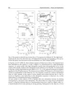
Fig. 3. Two different behaviors of the temperature starting at
0
x .
The second source of non-determinism comes from the continuous dynamics. The input

signal
u of the thermostat models the fluctuations in the outside temperature which we
cannot control. (Fig. 3 left) shows this continuous non-determinism. Starting from the initial
temperature
0
x , the system can generate a “tube” of infinite number of possible trajectories,
each of which corresponds to a different input signal
u . To capture uncertainty of sensors,
we define the first guard condition of the transition from 'on' to 'off' as an interval
[
]
,
MM
xx−ε +ε with 0
ε
 . This means that when the temperature enters this interval, the
thermostat can either turn the heater off immediately or keep it on for some time provided
Robust Control, Theory and Applications

28
that
M
xx≤+ε. (Fig. 3 right) illustrates this kind of non-determinism. Likewise, we define
the second guard condition of the transition from 'off' to 'on' as the interval
[
]
,
mm
xx−ε +ε .
Notice that in the thermostat model, the temperature does not change at the switching

points, and the reset maps are thus the identity functions.
Finally we define the two staying conditions of the 'on' and 'off' locations as
M
xx≤+ε
and
M
xx≥−εrespectively, meaning that the system can stay at a location while the
corresponding staying conditions are satisfied.
Example 2 (Bouncing Ball). Here, the ball (thought of as a point-mass) is dropped from an
initial height and bounces off the ground, dissipating its energy with each bounce. The ball
exhibits continuous dynamics between each bounce; however, as the ball impacts the
ground, its velocity undergoes a discrete change modeled after an inelastic collision. A
mathematical description of the bouncing ball follows. Let
1
:xh
=
be the height of the ball
and
2
:xh=

(Fig. 4). A hybrid system describing the ball is as follows:

2
0
():
.
gx
x
⎡

⎤
=
⎢
⎥
−γ
⎣
⎦
,
{
}
12
:: 0, 0Dxx x==≺
2
():
x
fx
g
⎡
⎤
=
⎢
⎥
−
⎣
⎦
,
{
}
1
:: 0\Cxx D=≥

. (2)
This model generates the sequence of hybrid arcs shown in (Fig. 5). However, it does not
generate the hybrid arc to which this sequence of solutions converges since the origin does
not belong to the jump set
D
. This situation can be remedied by including the origin in the
jump set
D . This amounts to replacing the jump set D by its closure. One can also replace
the flow set C by its closure, although this has no effect on the solutions.
It turns out that whenever the flow set and jump set are closed, the solutions of the corresponding
hybrid system enjoy a useful compactness property: every locally eventually bounded sequence of
solutions has a subsequence converging to a solution.


gy −=


?0

&

0 ≺hh =
)1,0(
.
∈
−=
+
γ
γ hh


g
h

Fig. 4. Diagram for the bouncing ball system

0
0
Time
h
h

Fig. 5. Solutions to the bouncing ball system
Consider the sequence of hybrid arcs depicted in (Fig. 5). They are solutions of a hybrid
“bouncing ball” model showing the position of the ball when dropped for successively
Robust Control of Hybrid Systems

29
lower heights, each time with zero velocity. The sequence of graphs created by these hybrid
arcs converges to a graph of a hybrid arc with hybrid time domain given by
{
}
0 ×
{nonnegative integers} where the value of the arc is zero everywhere on its domain. If
this hybrid arc is a solution then the hybrid system is said to have a “compactness”
property. This attribute for the solutions of hybrid systems is critical for robustness
properties. It is the hybrid generalization of a property that automatically holds for
continuous differential equations and difference equations, where nominal robustness of
asymptotic stability is guaranteed.
Solutions of hybrid systems are hybrid arcs that are generated in the following way: Let C

and
D be subsets of
n
ℜ
and let
f
, respectively
g
, be mappings fromC , respectively D ,
to
n
ℜ . The hybrid system :(,,,)HfgCD
=
can be written in the form

( )
()
x
f
xxC
x
g
xxD
+
=
∈
=
∈

(3)

The map f is called the “flow map”, the map
g
is called the “jump map”, the set C is called
the “flow set”, and the set
D is called the “jump set”. The state x may contain variables
taking values in a discrete set (logic variables), timers, etc. Consistent with such a situation is
the possibility that
CD∪ is a strict subset of
n
ℜ
. For simplicity, assume that
f
and
g
are
continuous functions. At times it is useful to allow these functions to be set-valued
mappings, which will denote by
F and G , in which case F and G should have a closed
graph and be locally bounded, and
F should have convex values.
In this case, we will write



xF xC
xGxD
+
∈
∈
∈

∈

(4)
A solution to the hybrid system (4) starting at a point
0
xCD
∈
∪ is a hybrid arc x with the
following properties:
1.

0
(0,0)xx= ;
2.
given
(,) sj domx∈
, if there exists s
τ
 such that
(,) jdomxτ∈
, then, for all
[
]
,ts∈τ,
(,)xt j C∈
and, for almost all
[
]
,ts
∈

τ ,
(,) ((,))xt j Fxt j∈

;
3.
given (,) tj domx∈ , if (, 1) tj domx+∈ then (,)xt j D
∈
and (, 1) ((,))xt j Gxt j+∈ .
Solutions from a given initial condition are not necessarily unique, even if the flow map is a
smooth function.
3. Approaches to analysis and design of hybrid control systems
The analysis and design tools for hybrid systems in this section are in the form of Lyapunov
stability theorems and LaSalle-like invariance principles. Systematic tools of this type are the
base of the theory of systems for purely of the continuous-time and discrete-time systems.
Some similar tools available for hybrid systems in (Michel, 1999) and (DeCarlo, 2000), the
tools presented in this section generalize their conventional versions of continuous-time and
discrete-time hybrid systems development by defining an equivalent concept of stability
and provide extensions intuitive sufficient conditions of stability asymptotically.
Robust Control, Theory and Applications

30
3.1 LaSalle-like invariance principles
Certain principles of invariance for the hybrid systems have been published in (Lygeros et
al., 2003) and (Chellaboina et al., 2002). Both results require, among other things, unique
solutions which is not generic for hybrid control systems. In (Sanfelice et al., 2005), the
general invariance principles were established that do not require uniqueness. The work in
(Sanfelice et al., 2005) contains several invariance results, some involving integrals of
functions, as for systems of continuous-time in (Byrnes & Martin, 1995) or (Ryan, 1998), and
some involving nonincreasing energy functions, as in work of LaSalle (LaSalle, 1967) or
(LaSalle, 1976). Such a result will be described here.

Suppose we can find a continuously differentiable function
:
n
V
ℜ
→ℜsuch that

( ): ( ), ( ) 0
( ): ( ( )) ( ) 0
c
d
ux Vx fx x C
ux Vgx Vx x D
=
∇≤∀∈
=
−≤ ∀∈
(5)
Consider (,)x ⋅⋅ a bounded solution with an unbounded hybrid time. Then there exists a value r in the
range V so that
x
tends to the largest weakly invariant set inside the set

(
)
(
)
1111
:() (0) (0)((0))
rcdd

MVr u u gu
−−−−
= ∩∪
(6)
where
1
(0)
d
u
−
: the set of points x satisfying () 0
d
ux
=
and
1
((0))
d
gu
−
corresponds to the set of
points
()gy where
1
(0)
d
yu
−
∈ .
The naive combination of continuous-time and discrete-time results would omit the

intersection with
1
((0))
d
gu
−
. This term, however, can be very useful for zeroing in set to
which trajectories converge.
3.2 Lyapunov stability theorems
Some preliminary results on the existence of the non-smooth Lyapunov function for the hybrid
systems published in (DeCarlo, 2000). The first results on the existence of smooth Lyapunov
functions, which are closely related to the robustness, published in (Cai et al., 2005). These
results required open basins of attraction, but this requirement has since been relaxed in (Cai et
al. 2007). The simplified discussion here is borrowed from this posterior work.
Let
O be an open subset of the state space containing a given compact set A and let
0
:
≥
ω→ℜO
be a continuous function which is zero for all xA
∈
, is positive otherwise,
which grows without limit as its argument grows without limit or near the limit
O . Such a
function is called a suitable indicator for the compact set
A in the open setO . An example of
such a function is the standard function on
n
ℜ

which is an appropriate indicator of origin.
More generally, the distance to a compact set
A is an appropriate indicator for all A on
n
ℜ .
Given an open set
O , an appropriate indicator
ω
and hybrid data (,,, )
f
gCD , a function
0
:V
≥
→ℜO
is called a smooth Lyapunov function for
(,,, ,,)fgCDω O
if it is smooth and
there exist functions
12
,
α
α belonging to the class-
∞
K , such as

12
1
(()) () (())
(),() ()

(()) ()
xVx x
Vx fx Vx
Vgx e Vx
−
α
ω≤ ≤αω
∇≤−
≤
x
xC
xD
∀
∈
∀∈
∀∈
∩
∩
O
O
O
(7)
Suppose that such a function exists, it is easy to verify that all solutions for the hybrid
system
(,,, )fgCDfrom
(
)
CD∩∪O satisfied
Robust Control of Hybrid Systems

31

(
)
1
12
( ( , )) ( ( (0,0))) ( , )
tj
xt j e x t j domx
−−
−
ω≤ααω ∀∈
(8)
In particular,
• (pre-stability of A ) for each 0
ε
 there exists 0
δ
 such that (0,0)xAB
∈
+δ implies,
for each generalized solution, that
(,)xt j A B
∈
+ε for all (,) tj domx
∈
, and
• (before attractive A onO ) any generalized solution from
(
)

CD∩∪O is bounded and if
its time domain is unbounded, so it converges to
A .
According to one of the principal results in (Cai et al., 2006)
there exists a smooth Lyapunov
function for
(,,, ,,)fgCD
ω
O if and only if the set A is pre-stable and pre-attractive on O and O is
forward invariant
(i.e.,
(
)
(0,0)xCD∈ ∩∪O implies (,)xt j
∈
O for all(,) tj domx
∈
).
One of the primary interests in inverse Lyapunov theorems is that they can be employed to
establish the robustness of the asymptotic stability of various types of perturbations.
4. Hybrid control application
In system theory in the 60s researchers were discussing mathematical frameworks so to
study systems with continuous and discrete dynamics. Current approaches to hybrid
systems differ with respect to the emphasis on or the complexity of the continuous and
discrete dynamics, and on whether they emphasize analysis and synthesis results or
analysis only or simulation only. On one end of the spectrum there are approaches to hybrid
systems that represent extensions of system theoretic ideas for systems (with continuous-
valued variables and continuous time) that are described by ordinary differential equations
to include discrete time and variables that exhibit jumps, or extend results to switching
systems. Typically these approaches are able to deal with complex continuous dynamics.

Their main emphasis has been on the stability of systems with discontinuities. On the other
end of the spectrum there are approaches to hybrid systems embedded in computer science
models and methods that represent extensions of verification methodologies from discrete
systems to hybrid systems. Several approaches to robustness of asymptotic stability and
synthesis of hybrid control systems are represented in this section.
4.1 Hybrid stabilization implies input-to-state stabilization
In the paper (Sontag, 1989) it has been shown, for continuous-time control systems, that
smooth stabilization involves smooth input-to-stat stabilization with respect to input
additive disturbances. The proof was based on converse Lyapunov theorems for
continuous-time systems. According to the indications of (Cai et al., 2006), and (Cai et al.
2007), the result generalizes to hybrid control systems via the converse Lyapunov theorem.
In particular, if we can find a hybrid controller, with the type of regularity used in sections
4.2 and 4.3, to achieve asymptotic stability, then the input-to-state stability with respect to
input additive disturbance can also be achieved.
Here, consider the special case where the hybrid controller is a logic-based controller where
the variable takes values in the logic of a finite set. Consider the hybrid control system

() ()( ) , q
:
( ) , q
qqqq q
qq
f
ud C Q
GDQ
q
+
⎧
ξ
=ξ+ηξ +υ ξ∈ ∈

⎪
⎪
=
⎨
ξ
⎡⎤
∈
ξξ∈∈
⎪
⎢⎥
⎪
⎣⎦
⎩

Η
(9)
Robust Control, Theory and Applications

32
where Q is a finite index set, for each qQ
∈
,
q
f
, :
n
qq
C
η
→ℜ are continuous functions,

q
C
and
q
D
are closed and
q
G
has a closed graph and is locally bounded. The signal
q
u
is the
control, and d is the disturbance, while
q
υ
is vector that is independent of the state, input,
and disturbance. Suppose
H is stabilizable by logic-based continuous feedback; that is, for
the case where 0d
=
, there exist continuous functions
q
k
defined on
q
C
such that, with
:()
qq
uk=ξ, the nonempty and compact set

{
}
qQ q
AAq
∈
=×∪
is pre-stable and globally pre-
attractive. Converse Lyapunov theorems can then be used to establish the existence of a
logic-based continuous feedback that renders the closed-loop system input-to-state stable
with respect to d . The feedback has the form

: () . () ()
T
qq q q
uk V
=
ξ−εη ξ∇ ξ
(10)
where 0ε
 and
()
q
V
ξ
is a smooth Lyapunov function that follows from the assumed
asymptotic stability when 0d
≡
. There exist class-
∞
K functions

1
α
and
2
α
such that, with
this feedback control, the following estimate holds:

()
()
(
)
()
2
2
11
12 1
(,)
(0,0)
max
( , ) max 2.exp . 0,0 ,
2.
qQ q
At j
Aq
tj t j d
∈
−−
∞
⎧

⎫
⎛⎞
υ
⎪
⎪
⎜⎟
ξ≤α−−αξ α
⎨
⎬
⎜⎟
ε
⎜⎟
⎪
⎪
⎝⎠
⎩⎭
(11)
where
(,)dom
:sup (,)
si d
ddsi
∈
∞
= .
4.2 Control Lyapunov functions
Although the control design using a continuously differentiable control-Lyapunov function
is well established for input-affine nonlinear control systems, it is well known that not all
controllable input-affine nonlinear control system function admits a continuously
differentiable control-Lyapunov function. A well known example in the absence of this

control-Lyapunov function is the so-called "Brockett", or "nonholonomic integrator".
Although this system does not allow continuously differentiable control Lyapunov function,
it has been established recently that admits a good "patchy" control-Lyapunov function.
The concept of control-Lyapunov function, which was presented in (Goebel et al., 2009), is
inspired not only by the classical control-Lyapunov function idea, but also by the approach
to feedback stabilization based on patchy vector fields proposed in (Ancona & Bressan,
1999). The idea of control-Lyapunov function was designed to overcome a limitation of
discontinuous feedbacks, such as those from patchy feedback, which is a lack of robustness
to measurement noise. In (Goebel et al., 2009) it has been demonstrated that any
asymptotically controllable nonlinear system admits a smooth patchy control-Lyapunov
function if we admit the possibility that the number of patches may need to be infinite. In
addition, it was shown how to construct a robust stabilizing hybrid feedback from a patchy
control-Lyapunov function. Here the idea when the number of patches is finite is outlined
and then specialized to the nonholonomic integrator.
Generally , a global patchy smooth control-Lyapunov function for the origin for the control
system
(,)xfxu=

in the case of a finite number of patches is a collection of functions
q
V
and
sets
q
Ω
and
q
′
Ω
where

{
}
: 1,,
q
Qm∈= … , such as
a.
for each qQ
∈
,
q
Ω
and
q
′
Ω
are open and
•

{
}
:\0
n
q
Q
qq
Q
q
∈∈
′
=ℜ = =

Ω
Ω
∪∪O
•
for each qQ∈ , the outward unit normal to
q
∂
Ω
is continuous on
(
)
rq
\
qr
′
∂
ΩΩ

∪∩O ,
Robust Control of Hybrid Systems

33
• for each qQ∈ ,
qq
′
⊂
Ω
Ω
∩ O
;

b.
for each qQ
∈
,
q
V is a smooth function defined on a neighborhood (relative to O )
of
q
Ω
.
c.
there exist a continuous positive definite function
α
and class-
∞
K functions
γ
and
γ
such that
•
()
(
)
()
q
xVx xγ≤ ≤γ
q
V
q

Q
∀
∈
,
(
)
\
qrqr
x
′
∈
ΩΩ

∪∩O
;
• for each qQ∈ and
(
)
\
q
r
q
r
x
′
∈
Ω
Ω

∪ there exists

,x
q
u such that
(),(, ,) ()
qx
Vx
f
xu
q
x∇≤−α

• for each qQ∈ and
(
)
\
qrqr
x
′
∈
ΩΩ

∪∩O there exists
,x
q
u such that
(),(, ,) ()
(),(, ,) ()
qx
qx
Vx

f
xu
q
x
nx
f
xu
q
x
∇≤−α
≤−α

where ( )
q
xnx denotes the outward unit normal to
q
∂
Ω
.
From this patchy control-Lyapunov function one can construct a robust hybrid feedback
stabilizer, at least when the set
{
}
,.(,) u
f
xu cυ≤
is convex for each real number
c
and every
real vector

υ , with the following data
:()
qq
ukx
=
,
(
)
\
qqrqr
C
′
=
ΩΩ

∪∩O
(12)
where
q
k is defined on
q
C , continuous and such that

()
( ), ( , ( )) 0.5 ( )
( ), ( , ( )) 0.5 ( ) \
qq q
qx qrkr
Vx fxkx x x C
nxfxkx x x

∇≤−α∀∈
′
≤− α ∀ ∈ ∂
ΩΩ

∪∩O
(13)
The jump set is given by

(
)
()
\
qqrqr
D
′
=
ΩΩ

∪∪ ∩OO
(14)
and the jump map is

{
}
(
)
{}
:
()

: \
rr
q
r
q
q
r
q
rQx rq x
Gx
rQx x
⎧
′′
∈∈ ∈
⎪
=
⎨
′
∈∈ ∈
⎪
⎩
Ω
ΩΩ
Ω
Ω

∩ ∪ ∩∩
∩
O, O
OO

(15)
With this control, the index increases with each jump except probably the first one. Thus, the
number of jumps is finite, and the state converges to the origin, which is also stable.
4.3 Throw-and-catch control
In ( Prieur, 2001), it was shown how to combine local and global state feedback to achieve
global stabilization and local performance. The idea, which exploits hysteresis switching
(Halbaoui et al., 2009b), is completely simple. Two continuous functions,
g
lobal
k and
local
k
are shown when the feedback ( )
global
uk x
=
render the origin of the control system
(,)xfxu=

globally asymptotically stable whereas the feedback ()
local
uk x
=
makes the
Robust Control, Theory and Applications

34
origin of the control system locally asymptotically stable with basin of attraction containing
the open set O , which contains the origin. Then we took
local

C a compact subset of the O
that contains the origin in its interior and one takes
g
lobal
D to be a compact subset of
local
C ,
again containing the origin in its interior and such that, when using the controller
local
k ,
trajectories starting in
g
lobal
D
never reach the boundary of
local
C (Fig. 6). Finally, the hybrid
control which achieves global asymptotic stabilization while using the controller
q
k for
small signals is as follows

{
}
{}
: ( ) : :
( , ) : toggle ( ) D : :
qq
q
ukx C (x,q)xC

gqx q (x,q) x D
==∈
==∈
(16)
In the problem of uniting of local and global controllers, one can view the global controller
as a type of "bootstrap" controller that is guaranteed to bring the system to a region where
another controller can control the system adequately.
A prolongation of the idea of combine local and global controllers is to assume the existence
of continuous bootstrap controller that is guaranteed to introduce the system, in finite time,
in a vicinity of a set of points, not simply a vicinity of the desired final destination (the
controller doesn’t need to be able to maintain the state in this vicinity); moreover, these sets
of points form chains that terminate at the desired final destination and along which
controls are known to steer (or “throw”) form one point in the chain at the next point in the
chain. Moreover, in order to minimize error propagation along a chain, a local stabilizer is
known for each point, except perhaps those points at the start of a chain. Those can be
employed “to catch” each jet.

.
global
D

local
C

Trajectory due to local
controller


Fig. 6. Combining local and global controllers
4.4 Supervisory control

In this section, we review the supervisory control framework for hybrid systems. One of the
main characteristics of this approach is that the plant is approximated by a discrete-event
system and the design is carried out in the discrete domain. The hybrid control systems in
the supervisory control framework consist of a continuous (state, variable) system to be
controlled, also called the plant, and a discrete event controller connected to the plant via an
interface in a feedback configuration as shown in (Fig. 7). It is generally assumed that the
dynamic behavior of the plant is governed by a set of known nonlinear ordinary differential
equations

() ((),())xt f xt rt
=

(17)
Robust Control of Hybrid Systems

35
where
n
x ∈ℜis the continuous state of the system and
m
r
∈
ℜ is the continuous control
input. In the model shown in (Fig. 7), the plant contains all continuous components of the
hybrid control system, such as any conventional continuous controllers that may have been
developed, a clock if time and synchronous operations are to be modeled, and so on. The
controller is an event driven, asynchronous discrete event system (DES), described by a
finite state automaton. The hybrid control system also contains an interface that provides
the means for communication between the continuous plant and the DES controller.

Discrete
Envent system
DES Supervisor
Event
recognizer
Control
Switch




Controlled s
y
stem
Continuous variable
system
Interface


Fig. 7. Hybrid system model in the supervisory control framework.

)(
1
xh

)(
4
xh

)(

2
xh

)(
3
xh

X

Fig. 8. Partition of the continuous state space.
The interface consists of the generator and the actuator as shown in (Fig. 7). The generator
has been chosen to be a partitioning of the state space (see Fig. 8). The piecewise continuous
command signal issued by the actuator is a staircase signal as shown in (Fig. 9), not unlike
the output of a zero-order hold in a digital control system. The interface plays a key role in
determining the dynamic behavior of the hybrid control system. Many times the partition of
the state space is determined by physical constraints and it is fixed and given.
Methodologies for the computation of the partition based on the specifications have also
been developed.
In such a hybrid control system, the plant taken together with the actuator and generator,
behaves like a discrete event system; it accepts symbolic inputs via the actuator and
produces symbolic outputs via the generator. This situation is somewhat analogous to the

Robust Control, Theory and Applications

36

time

]1[
c

t

]2[
c
t

]3[
c
t


Fig. 9. Command signal issued by the interface.
way a continuous time plant, equipped with a zero-order hold and a sampler, “looks” like a
discrete-time plant. The DES which models the plant, actuator, and generator is called the
DES plant model. From the DES controller's point of view, it is the DES plant model which
is controlled.
The DES plant model is an approximation of the actual system and its behavior is an
abstraction of the system's behavior. As a result, the future behavior of the actual continuous
system cannot be determined uniquely, in general, from knowledge of the DES plant state
and input. The approach taken in the supervisory control framework is to incorporate all the
possible future behaviors of the continuous plant into the DES plant model. A conservative
approximation of the behavior of the continuous plant is constructed and realized by a finite
state machine. From a control point of view this means that if undesirable behaviors can be
eliminated from the DES plant (through appropriate control policies) then these behaviors
will be eliminated from the actual system. On the other hand, just because a control policy
permits a given behavior in the DES plant, is no guarantee that that behavior will occur in
the actual system.
We briefly discuss the issues related to the approximation of the plant by a DES plant model.
A dynamical system
∑

can be described as a triple ;;TWBwith T ⊆ℜthe time axis, W the
signal space, and
T
BW⊂ (the set of all functions
:fT W→
) the behavior. The behavior of the
DES plant model consists of all the pairs of plant and control symbols that it can generate.
The time axis
T represents here the occurrences of events. A necessary condition for the
DES plant model to be a valid approximation of the continuous plant is that the behavior of
the continuous plant model
c
B is contained in the behavior of the DES plant model, i.e.
cd
BB⊆ .
The main objective of the controller is to restrict the behavior of the DES plant model in
order to specify the control specifications. The specifications can be described by a
behavior
s
p
ec
B . Supervisory control of hybrid systems is based on the fact that if undesirable
behaviors can be eliminated from the DES plant then these behaviors can likewise be eliminated from
the actual system. This is described formally by the relation

d s spec c s spec
BBB BBB⊆⇒ ⊆∩∩
(18)
and is depicted in (Fig. 10). The challenge is to find a discrete abstraction with behavior B
d

which is a approximation of the behavior B
c
of the continuous plant and for which is
possible to design a supervisor in order to guarantee that the behavior of the closed loop
system satisfies the specifications B
spec
. A more accurate approximation of the plant's
behavior can be obtained by considering a finer partitioning of the state space for the
extraction of the DES plant.
Robust Control of Hybrid Systems

37
spec
B

s
B

d
B

c
B


Fig. 10. The DES plant model as an approximation.
An interesting aspect of the DES plant's behavior is that it is distinctly nondeterministic.
This fact is illustrated in (Fig.11). The figure shows two different trajectories generated by
the same control symbol. Both trajectories originate in the same DES plant state

1
p

. (Fig.11)
shows that for a given control symbol, there are at least two possible DES plant states that
can be reached from
1
p

. Transitions within a DES plant will usually be nondeterministic
unless the boundaries of the partition sets are invariant manifolds with respect to the vector
fields that describe the continuous plant.

A

B

1
~
X

2
~
X

2
~
P

3

~
P

1
~
P


Fig. 11. Nondeterminism of the DES plant model.
There is an advantage to having a hybrid control system in which the DES plant model is
deterministic. It allows the controller to drive the plant state through any desired sequence
of regions provided, of course, that the corresponding state transitions exist in the DES plant
model. If the DES plant model is not deterministic, this will not always be possible. This is
because even if the desired sequence of state transitions exists, the sequence of inputs which
achieves it may also permit other sequences of state transitions. Unfortunately, given a
continuous-time plant, it may be difficult or even impossible to design an interface that
leads to a DES plant model which is deterministic. Fortunately, it is not generally necessary
to have a deterministic DES plant model in order to control it. The supervisory control
problem for hybrid systems can be formulated and solved when the DES plant model is
nondeterministic. This work builds upon the frame work of supervisory control theory used
in (Halbaoui et al., 2008) and (Halbaoui et al., 2009a).
5. Robustness to perturbations
In control systems, several perturbations can occur and potentially destroy the good
behavior for which the controller was designed for. For example, noise in the measurements
Robust Control, Theory and Applications

38
of the state taken by controller arises in all implemented systems. It is also common that
when a controller is designed, only a simplified model of the system to control exhibiting
the most important dynamics is considered. This simplifies the control design in general.

However, sensors/actuators that are dynamics unmodelled can substantially affect the
behavior of the system when in the loop. In this section, it is desired that the hybrid
controller provides a certain degree of robustness to such disturbances. In the following
sections, general statements are made in this regard.
5.1 Robustness via filtered measurements
In this section, the case of noise in the measurements of the state of the nonlinear system is
considered. Measurement noise in hybrid systems can lead to nonexistence of solutions.
This situation can be corrected, at least for the small measurement noise, if under global
existence of solutions,
c
C and
c
D always “overlap” while ensuring that the stability
properties still hold. The "overlap" means that for every O
ξ
∈ , either
c
eCξ+ ∈
or
c
eDξ+ ∈

all or small e . There exist generally always inflations of C and
D that preserve the
semiglobal practices asymptotic stability, but they do not guarantee the existence of
solutions for small measurement noise.
Moreover, the solutions are guaranteed to exist for any locally bounded measurement noise
if the measurement noise does not appear in the flow and jump sets. This can be carried out
by filtering measures. (Fig. 12) illustrates this scenario. The state
x is corrupted by the noise

e and the hybrid controller
c
H measures a filtered version of xe
+
.

Filter
Hybrid system

e

+

x

u

+
Controller
k

f
x


Fig. 12. Closed-loop system with noise and filtered measurements.
The filter used for the noisy output
y
xe
=

+ is considered to be linear and defined by the
matrices
f
A ,
f
B , and
f
L , and an additional parameter 0
f
ε
> . It is designed to be
asymptotically stable. Its state is denoted by
f
x which takes value in
f
n
R . At the jumps,
f
x
is given to the current value of
y
. Then, the filter has flows given by
,
ff ff f
xAxB
y
ε
=+

(19)

and jumps given by

1
.
fffff
xABxB
y
+
−
=+
(20)
The output of the filter replaces the state x in the feedback law. The resulting closed-loop
system can be interpreted as family of hybrid systems which depends on the parameter
f
ε .
It is denoted by
f
cl
H
ε
and is given by
Robust Control of Hybrid Systems

39
:
f
cl
H
ε

1
((,))
(,)
()
(,)
()
pffc
ccffc
ff ff f
ccffc
fff
xfx Lxx
xfLxx
xAxBxe
xx
xGLxx
xABxe
+
+
+−
⎧
⎫
=+κ
⎪
⎪
⎪
=
⎪
⎬
⎪

⎪
ε= + +
⎪
⎪
⎭
⎪
⎨
⎫
=
⎪
⎪
⎪
⎪
∈
⎬
⎪
⎪
⎪
=− +
⎪
⎪
⎭
⎩




(,)
(,)
ff

cc
ff
cc
Lx x C
Lx x D
∈
∈
(21)
5.2 Robustness to sensor and actuator dynamics
This section reviews the robustness of the closed-loop
cl
H when additional dynamics,
coming from sensors and actuators, are incorporated. (Fig. 13) shows the closed loop
cl
H
with two additional blocks: a model for the sensor and a model for the actuator. Generally,
to simplify the controller design procedure, these dynamics are not included in the model of
the system ( , )
p
x
f
xu=

when the hybrid controller
c
H is conceived. Consequently, it is
important to know whether the stability properties of the closed-loop system are preserved,
at least semiglobally and practically, when those dynamics are incorporated in the closed
loop.
The sensor and actuator dynamics are modeled as stable filters. The state of the filter which

models the sensor dynamics is given by
s
n
s
xR∈ with matrices (,,)
sss
A
BL , the state of the
filter that models the actuator dynamics is given by
a
n
a
xR∈ with matrices(,,)
aaa
A
BL , and
0
d
ε> is common to both filters.
Augmenting
cl
H by adding filters and temporal regularization leads to a family
d
cl
H
ε
given
as follows

*

(, )
(,)
( , ) or
()
(,)
:
( , )

0
d
paa
ccssc
ss c c
ds ss s
da aa a ss c
cl
ccssc
ss
aa
xfxLx
xfLxx
Lx x C
xAxBxe
xAxBLxx
H
xx
xGLxx
xx
xx
ε

+
+
+
+
+
=
⎫
⎪
=
⎪
⎪
τ=−τ+τ ∈ τ≤τ
⎬
⎪
ε= + +
⎪
⎪
ε= +κ
⎭
⎫
=
∈
=
=
τ=






( , ) and
ss c c
Lx x D
⎧
⎪
⎪
⎪
⎪
⎪
⎪
⎪
⎪
⎨
⎪
⎪
⎪
⎪
⎪
⎪
⎪
∈τ≥τ
⎬
⎪
⎪
⎪
⎪
⎪
⎪
⎪

⎭
⎩
(22)
where
*
τ is a constant satisfying
*
τ
>τ.
The following result states that for fast enough sensors and actuators, and small enough
temporal regularization parameter, the compact set
A is semiglobally practically
asymptotically stable.
Robust Control, Theory and Applications

40

Sensor
Actuator
Hybrid system

e

+

x

u

+

Controller
k

s
x


Fig. 13. Closed-loop system with sensor and actuator dynamics.
5.3 Robustness to sensor dynamics and smoothing
In many hybrid control applications, the state of the controller is explicitly given as a
continuous state
ξ
and a discrete state
{
}
:1, ,
q
Qn∈= , that is,
:[ ]
T
c
x
q
=ξ
. Where this is the
case and the discrete state
q
chooses a different control law to be applied to the system for
for various values of

q
, then the control law generated by the hybrid controller
c
H can
have jumps when
q
changes. In many scenarios, it is not possible for the actuator to switch
between control laws instantly. In addition, particularly when the control law
(· , · , )qκ is
continuous for each
qQ
∈
, it is desired to have a smooth transition between them when
q

changes.

Sensor
Smoothing
Hybrid system

u

Controller
n
k

s
x

1
k

q


Fig. 14. Closed-loop system with sensor dynamics and control smoothing.
(Fig. 14) shows the closed-loop system, noted that
d
cl
H
ε
, resulting from adding a block that
makes the smooth transition between control laws indexed by
q
and indicated by
q
κ . The
smoothing control block is modeled as a linear filter for the variable
q
. It is defined by the
parameter
u
ε
and the matrices
(,,)
uuu
A
BL
.

The output of the control smoothing block is given by

(, , ) ( )(, ,)
cuu quu c
qQ
xx Lx Lx xx
q
∈
α=λκ
∑
(23)
where for each , : [0,1]
q
qQ R
∈
λ→ , is continuous and ( ) 1
q
q
λ
= . Note that the output is
such that the control laws are smoothly “blended” by the function
q
λ
.
In addition to this block, a filter modeling the sensor dynamics is also incorporated as in
section 5.2. The closed loop
f
cl
H
ε

can be written as
Robust Control of Hybrid Systems

41

*
((,,))
(,)
0
(,) or
()
:
(,)
(
0
f
pcuu
ccssc
ss c c
us ss s
uu uu u
cl
cssc
ss s
uu
xfx xxLx
xfLxx
q
Lx x C
xAxBx

xAxBq
xx
H
GLxx
q
xx L
xx
+
ε
+
+
+
+
+
+
=+α
⎫
⎪
=
⎪
⎪
=
⎪
∈τ≤τ
⎬
τ=−τ+τ
⎪
⎪
ε= +
⎪

⎪
ε= +
⎭
⎫
=
⎪
⎪
⎡⎤
ξ
⎪
∈
⎢⎥
⎪
⎢⎥
⎣⎦
⎪
⎪
=
⎬
⎪
=
⎪
⎪
τ=
⎪
⎪
⎪
⎭








,) and
sc c
xx D
⎧
⎪
⎪
⎪
⎪
⎪
⎪
⎪
⎪
⎪
⎪
⎪
⎨
⎪
⎪
⎪
⎪
⎪
∈τ≥τ
⎪
⎪
⎪

⎪
⎪
⎪
⎩
(24)
6. Conclusion
In this chapter, a dynamic systems approach to analysis and design of hybrid systems has
been continued from a robust control point of view. Stability and convergence tools for
hybrid systems presented include hybrid versions of the traditional Lyapunov stability
theorem and of LaSalle’s invariance principle.
The robustness of asymptotic stability for classes of closed-loop systems resulting from
hybrid control was presented. Results for perturbations arising from the presence of
measurement noise, unmodeled sensor and actuator dynamics, control smoothing.
It is very important to have good software tools for the simulation, analysis and design of
hybrid systems, which by their nature are complex systems. Researchers have recognized
this need and several software packages have been developed.
7. References
Rajeev, A.; Thomas, A. & Pei-Hsin, H.(1993). Automatic symbolic verification of embedded
systems, In IEEE Real-Time Systems Symposium, 2-11, DOI:
10.1109/REAL.1993.393520 .
Dang, T. (2000). Vérification et Synthèse des Systèmes Hybrides. PhD thesis, Institut National
Polytechnique de Grenoble.
Girard, A. (2006). Analyse algorithmique des systèmes hybrides. PhD thesis, Universitè Joseph
Fourier (Grenoble-I).
Ancona, F. & Bressan, A. (1999). Patchy vector fields and asymptotic stabilization, ESAIM:
Control, Optimisation and Calculus of Variations, 4:445–471, DOI:
10.1051/cocv:2004003.
Byrnes, C. I. & Martin, C. F. (1995). An integral-invariance principle for nonlinear systems, IEEE
Transactions on Automatic Control, 983–994, ISSN: 0018-9286.
Robust Control, Theory and Applications

42
Cai, C.; Teel, A. R. & Goebel, R. (2007). Results on existence of smooth Lyapunov functions for
asymptotically stable hybrid systems with nonopen basin of attraction, submitted to the
2007 American Control Conference, 3456 – 3461, ISSN: 0743-1619.
Cai, C.; Teel, A. R. & Goebel, R. (2006). Smooth Lyapunov functions for hybrid systems Part I:
Existence is equivalent to robustness & Part II: (Pre-)asymptotically stable compact
sets, 1264-1277, ISSN 0018-9286.
Cai, C.; Teel, A. R. & Goebel, R. (2005). Converse Lyapunov theorems and robust asymptotic
stability for hybrid systems, Proceedings of 24th American Control Conference, 12–17,
ISSN: 0743-1619.
Chellaboina, V.; Bhat, S. P. & HaddadWH. (2002). An invariance principle for nonlinear hybrid
and impulsive dynamical systems. Nonlinear Analysis, Chicago, IL, USA, 3116 –
3122,ISBN: 0-7803-5519-9.
Goebel, R.; Prieur, C. & Teel, A. R. (2009). smooth patchy control Lyapunov functions.
Automatica (Oxford) Y, 675-683 ISSN : 0005-1098.
Goebel, R. & Teel, A. R. (2006). Solutions to hybrid inclusions via set and graphical convergence
with stability theory applications. Automatica, 573–587, DOI:
10.1016/j.automatica.2005.12.019.
LaSalle, J. P. (1967). An invariance principle in the theory of stability, in Differential equations and
dynamical systems. Academic Press, New York.
LaSalle, J. P. (1976) The stability of dynamical systems. Regional Conference Series in Applied
Mathematics, SIAM ISBN-13: 978-0-898710-22-9.
Lygeros, J.; Johansson, K. H., Simi´c, S. N.; Zhang, J. & Sastry, S. S. (2003). Dynamical
properties of hybrid automata. IEEE Transactions on Automatic Control, 2–17 ,ISSN:
0018-9286.
Prieur, C. (2001). Uniting local and global controllers with robustness to vanishing noise,
Mathematics Control, Signals, and Systems, 143–172, DOI: 10.1007/PL00009880
Ryan, E. P. (1998). An integral invariance principle for differential inclusions with applications in
adaptive control. SIAM Journal on Control and Optimization, 960–980, ISSN 0363-

0129.
Sanfelice, R. G.; Goebel, R. & Teel, A. R. (2005). Results on convergence in hybrid systems via
detectability and an invariance principle. Proceedings of 2005 American Control
Conference, 551–556, ISSN: 0743-1619.
Sontag, E. (1989). Smooth stabilization implies coprime factorization. IEEE Transactions on
Automatic Control, 435–443, ISSN: 0018-9286.
DeCarlo, R.A.; Branicky, M.S.; Pettersson, S. & Lennartson, B.(2000). Perspectives and results
on the stability and stabilizability of hybrid systems. Proc. of IEEE, 1069–1082, ISSN:
0018-9219.
Michel, A.N.(1999). Recent trends in the stability analysis of hybrid dynamical systems. IEEE
Trans. Circuits Syst. – I. Fund. Theory Appl., 120–134,ISSN: 1057-7122.
Halbaoui, K.; Boukhetala, D. and Boudjema, F.(2008). New robust model reference adaptive
control for induction motor drives using a hybrid controller.International Symposium on
Power Electronics, Electrical Drives, Automation and Motion, Italy, 1109 - 1113
ISBN: 978-1-4244-1663-9.
Halbaoui, K.; Boukhetala, D. and Boudjema, F.(2009a). Speed Control of Induction Motor
Drives Using a New Robust Hybrid Model Reference Adaptive Controller. Journal of
Applied Sciences, 2753-2761, ISSN:18125654.
Halbaoui, K.; Boukhetala, D. and Boudjema, F.(2009b). Hybrid adaptive control for speed
regulation of an induction motor drive,
Archives of Control Sciences,V2.
3
Robust Stability and Control of
Linear Interval Parameter Systems
Using Quantitative (State Space) and
Qualitative (Ecological) Perspectives
Rama K. Yedavalli and Nagini Devarakonda
The Ohio State University
United States of America
1. Introduction

The problem of maintaining the stability of a nominally stable linear time invariant system
subject to linear perturbation has been an active topic of research for quite some time. The
recent published literature on this `robust stability’ problem can be viewed mainly from two
perspectives, namely i) transfer function (input/output) viewpoint and ii) state space
viewpoint. In the transfer function approach, the analysis and synthesis is essentially carried
out in frequency domain, whereas in the state space approach it is basically carried out in
time domain. Another perspective that is especially germane to this viewpoint is that the
frequency domain treatment involves the extensive use of `polynomial’ theory while that of
time domain involves the use of ‘matrix’ theory. Recent advances in this field are surveyed
in [1]-[2].
Even though in typical control problems, these two theories are intimately related and
qualitatively similar, it is also important to keep in mind that there are noteworthy
differences between these two approaches (‘polynomial’ vs ‘matrix’) and this chapter (both
in parts I and II) highlights the use of the direct matrix approach in the solution to the robust
stability and control design problems.
2. Uncertainty characterization and robustness
It was shown in [3] that modeling errors can be broadly categorized as i) parameter
variations, ii) unmodeled dynamics iii) neglected nonlinearities and finally iv) external
disturbances. Characterization of these modeling errors in turn depends on the
representation of dynamic system, namely whether it is a frequency domain, transfer
function framework or time domain state space framework. In fact, some of these can be
better captured in one framework than in another. For example, it can be argued
convincingly that real parameter variations are better captured in time domain state space
framework than in frequency domain transfer function framework. Similarly, it is intuitively
clear that unmodeled dynamics errors can be better captured in the transfer function
framework. By similar lines of thought, it can be safely agreed that while neglected
nonlinearities can be better captured in state space framework, neglected disturbances can
Robust Control, Theory and Applications

44

be captured with equal ease in both frameworks. Thus it is not surprising that most of the
robustness studies of uncertain dynamical systems with real parameter variations are being
carried out in time domain state space framework and hence in this chapter, we emphasize
the aspect of robust stabilization and control of linear dynamical systems with real
parameter uncertainty.
Stability and performance are two fundamental characteristics of any feedback control
system. Accordingly, stability robustness and performance robustness are two desirable
(sometimes necessary) features of a robust control system. Since stability robustness is a
prerequisite for performance robustness, it is natural to address the issue of stability
robustness first and then the issue of performance robustness.
Since stability tests are different for time varying systems and time invariant systems, it is
important to pay special attention to the nature of perturbations, namely time varying
perturbations versus time invariant perturbations, where it is assumed that the nominal
system is a linear time invariant system. Typically, stability of linear time varying systems is
assessed using Lyapunov stability theory using the concept of quadratic stability whereas
that of a linear time invariant system is determined by the Hurwitz stability, i.e. by the
negative real part eigenvalue criterion. This distinction about the nature of perturbation
profoundly affects the methodologies used for stability robustness analysis.
Let us consider the following linear, homogeneous, time invariant asymptotically stable
system in state space form subject to a linear perturbation E:

(
)
00
(0)xAEx x x
=
+=

(1)
where A

0
is an n×n asymptotically stable matrix and E is the error (or perturbation) matrix.
The two aspects of characterization of the perturbation matrix E which have significant
influence on the scope and methodology of any proposed analysis and design scheme are i)
the temporal nature and ii) the boundedness nature of E. Specifically, we can have the
following scenario:
i.
Temporal Nature:
Time invariant error
E = constant
vs
Time varying error
E = E(t)
ii.
Boundedness Nature:
Unstructured
(Norm bounded)
vs
Structured
(Elemental bounds)
The stability robustness problem for linear time invariant systems in the presence of linear
time invariant perturbations (i.e. robust Hurwitz invariance problem) is basically addressed
by testing for the negativity of the real parts of the eigenvalues (either in frequency domain
or in time domain treatments), whereas the time varying perturbation case is known to be
best handled by the time domain Lyapunov stability analysis. The robust Hurwitz
invariance problem has been widely discussed in the literature essentially using the
polynomial approach [4]-[5]. In this section, we address the time varying perturbation case,
mainly motivated by the fact that any methodology which treats the time varying case can
always be specialized to the time invariant case but not vice versa. However, we pay a price
for the same, namely conservatism associated with the results when applied to the time

invariant perturbation case. A methodology specifically tailored to time invariant
perturbations is discussed and included by the author in a separate publication [6].
Robust Stability and Control of Linear Interval Parameter Systems
Using Quantitative (State Space) and Qualitative (Ecological) Perspectives

45
It is also appropriate to discuss, at this point, the characterization with regard to the
boundedness of the perturbation. In the so called ‘unstructured’ perturbation, it is assumed
that one cannot clearly identify the location of the perturbation within the nominal matrix
and thus one has simply a bound on the norm of the perturbation matrix. In the ‘structured’
perturbation, one has information about the location(s) of the perturbation and thus one can
think of having bounds on the individual elements of the perturbation matrix. This
approach can be labeled as ‘Elemental Perturbation Bound Analysis (EPBA)’. Whether
‘unstructured’ norm bounded perturbation or ‘structured’ elemental perturbation is
appropriate to consider depends very much on the application at hand. However, it can be
safely argued that ‘structured’ real parameter perturbation situation has extensive
applications in many engineering disciplines as the elements of the matrices of a linear state
space description contain parameters of interest in the evolution of the state variables and it
is natural to look for bounds on these real parameters that can maintain the stability of the
state space system.
3. Robust stability and control of linear interval parameter systems under
state space framework
In this section, we first give a brief account of the robust stability analysis techniques in 3.1
and then in subsection 3.2 we discuss the robust control design aspect.
3.1 Robust stability analysis
The starting point for the problem at hand is to consider a linear state space system
described by
[
]
0

() ()xt A Ext=+


where x is an n dimensional state vector, asymptotically stable matrix and E is the
‘perturbation’ matrix. The issue of ‘stability robustness measures’ involves the
determination of bounds on E which guarantee the preservation of stability of (1). Evidently,
the characterization of the perturbation matrix E has considerable influence on the derived
result. In what follows, we summarize a few of the available results, based on the
characterization of E.
1. Time varying (real) unstructured perturbation with spectral norm: Sufficient bound
For this case, the perturbation matrix E is allowed to be time varying, i.e. E(t) and a bound
on the spectral norm (
(
)
max
()Et
σ
where σ(·) is the singular value of (·)) is derived. When a
bound on the norm of E is given, we refer to it as ‘unstructured’ perturbation. This norm
produces a spherical region in parameter space. The following result is available for this
case [7]-[8]:

()
max
max
1
()
()
Et
P

σ
σ
<
(2)
where P is the solution to the Lyapunov matrix

00
20
T
PA A P I
+
+=
(3)
See Refs [9],[10],[11] for results related to this case.
Robust Control, Theory and Applications

46
2. Time varying (real) structured variation
Case 1: Independent variations (sufficient bound) [12]-[13]

max
() ()
i
j
ti
j
i
j
Et Et
ε

≤
∀=
(4)
i
j
i
j
Max
ε
ε
=


()
max
1
i
j
ei
j
me
s
U
PU
ε
σ
< (5)
where P satisfies equation (3) and U
oij
= ε

ij
/ ε. For cases when ε
ij
are not known, one can take
U
eij
= |A
oij
|/|A
oij
|
max
. (·)
m
denotes the matrix with all modulus elements and (·)
s
denotes the
symmetric part of (·).
3. Time invariant, (real) structured perturbation E
ij
= Constant
Case i: Independent Variations [13]-[15]: (Sufficient Bounds). For this case, E can be
characterized as

12
ESDS
=
(6)
where S
1

and S
2
are constant, known matrices and |D
ij
| ≤ d
ij
d with d
ij
≥ 0 are given and d > 0
is the unknown. Let U be the matrix elements U
ij
= d
ij
. Then the bound on d is given by [13]

()
1
201
0
1
J
Q
Sup
m
d
SjIA S U
ω
μ
μ
ω

−
>
<==
⎛⎞
⎡⎤
−
⎜⎟
⎢⎥
⎣⎦
⎝⎠
(7)
Notice that the characterization of E (with time invariant) in (4) is accommodated by the
characterization in [15]. ρ(·) is the spectral radius of (·).
Case ii: Linear Dependent Variation: For this case, E is characterized (as in (6) before), by

1
r
ii
i
EE
β
=
=
∑
(8)
and bounds on |β
i
| are sought. Improved bounds on |β
i
| are presented in [6].

This type of representation represents a ‘polytope of matrices’ as discussed in [4]. In this
notation, the interval matrix case (i.e. the independent variation case) is a special case of the
above representation where Ei contains a single nonzero element, at a different place in the
matrix for different i.
For the time invariant, real structured perturbation case, there are no computationally
tractable necessary and sufficient bounds either for polytope of matrices or for interval
matrices (even for a 2 x 2 case). Even though some derivable necessary and sufficient
conditions are presented in [16] for any general variation in E (not necessarily linear
dependent and independent case), there are no easily computable methods available to
determine the necessary and sufficient bounds at this stage of research. So most of the
research, at this point of time, seems to aim at getting better (less conservative) sufficient
bounds. The following example compares the sufficient bounds given in [13]-[15] for the
linear dependent variation case.
Robust Stability and Control of Linear Interval Parameter Systems
Using Quantitative (State Space) and Qualitative (Ecological) Perspectives

47
Let us consider the example given in [15] in which the perturbed system matrix is given by
()
11
02
121
201
03 0
114
kk
ABKC k
kkk
−+ −+
⎡

⎤
⎢
⎥
+= −+
⎢
⎥
⎢
⎥
−+ −+ −+
⎣
⎦

Taking the nominally stable matrix to be
0
20 1
030
114
A
−
−
⎡
⎤
⎢
⎥
=−
⎢
⎥
⎢
⎥
−

−−
⎣
⎦

the error matrix with k
1
and k
2
as the uncertain parameters is given by
11 22
EkE kE=+
where
1
101
000
101
E
⎡
⎤
⎢
⎥
=
⎢
⎥
⎢
⎥
⎣
⎦
and
2

000
010
010
E
⎡
⎤
⎢
⎥
=
⎢
⎥
⎢
⎥
⎣
⎦

The following are the bounds on |k
1
| and |k
2
| obtained by [15] and the proposed method.

µ
y
µ
Q
ZK [14] µ
d
[6]
0.815 0.875 1.55 1.75

3.2 Robust control design for linear systems with structured uncertainty
Having discussed the robustness analysis issue above, we now switch our attention to the
robust control design issue. Towards this direction, we now present a linear robust control
design algorithm for linear deterministic uncertain systems whose parameters vary within
given bounded sets. The algorithm explicitly incorporates the structure of the uncertainty
into the design procedure and utilizes the elemental perturbation bounds developed above.
A linear state feedback controller is designed by parameter optimization techniques to
maximize (in a given sense) the elemental perturbation bounds for robust stabilization.
There is a considerable amount of literature on the aspect of designing linear controllers for
linear tine invariant systems with small parameter uncertainty. However, for uncertain
systems whose dynamics are described by interval matrices (i.e., matrices whose elements
are known to vary within a given bounded interval), linear control design schemes that
guarantee stability have been relatively scarce. Reference [17] compares several techniques
for designing linear controllers for robust stability for a class of uncertain linear systems.
Among the methods considered are the standard linear quadratic regulator (LQR) design,
Guaranteed Cost Control (GCC) method of [18], Multistep Guaranteed Cost Control
(MGCC) of [17]. In these methods, the weighting on state in a quadratic cost function and
the Riccati equation are modified in the search for an appropriate controller. Also, the
parameter uncertainty is assumed to enter linearly and restrictive conditions are imposed on
the bounding sets. In [18], norm inequalities on the bounding sets are given for stability but
Robust Control, Theory and Applications

48
they are conservative since they do not take advantage of the system structure. There is no
guarantee that a linear state feedback controller exists. Reference [19] utilizes the concept of
‘Matching conditions (MC)’ which in essence constrain the manner in which the uncertainty
is permitted to enter into the dynamics and show that a linear state feedback control that
guarantees stability exists provided the uncertainty satisfies matching conditions. By this
method large bounding sets produce large feedback gains but the existence of a linear
controller is guaranteed. But no such guarantee can be given for general ‘mismatched’

uncertain systems. References [20] and [21] present methods which need the testing of
definiteness of a Lyapunov matrix obtained as a function of the uncertain parameters. In the
multimodel theory approach, [22] considers a discrete set of points in the parameter
uncertainty range to establish the stability. This paper addresses the stabilization problem
for a continuous range of parameters in the uncertain parameter set (i.e. in the context of
interval matrices). The proposed approach attacks the stability of interval matrix problem
directly in the matrix domain rather than converting the interval matrix to interval
polynomials and then testing the Kharitonov polynomials.
Robust control design using perturbation bound analysis [23],[24]
Consider a linear, time invariant system described by
xAxBu
=
+


0
(0)xx
=

Where
x is 1n × state vector, the control u is 1m
×
. The matrix pair (,)AB is assumed to
be completely controllable.
U=Gx
For this case, the nominal closed loop system matrix is given by
AABG=+ ,
1
0
T

c
RBK
G
ρ
−
−
=

and
1
0
0
TT
c
R
KA A K KB B K Q
ρ
−
+
−+=
and
A
is asymptotically stable.
Here
G is the Riccati based control gain where Q,and R
0
are any given weighting matrices
which are symmetric, positive definite and
ρ
c

is the design variable.
The main interest in determining
G is to keep the nominal closed loop system stable. The
reason Riccati approach is used to determine
G is that it readily renders (A+BG)
asymptotically stable with the above assumption on
Q and R
0
.
Now consider the perturbed system with linear time varying perturbations
E
A
(t) and E
B
(t)
respectively in matrices
A and B
i.e.,
[
]
[
]
() () () ()
AB
x AEtxt BEtut=+ ++


Let Δ
A and ΔB be the perturbation matrices formed by the maximum modulus deviations
expected in the individual elements of matrices

A and B respectively. Then one can write
aea
beb
AU
BU
Δε
Δε
=
=
(Absolute variation)
Robust Stability and Control of Linear Interval Parameter Systems
Using Quantitative (State Space) and Qualitative (Ecological) Perspectives

49
where ε
a
is the maximum of all the elements in ΔA and ε
b
is the maximum of all elements in
ΔB. Then the total perturbation in the linear closed loop system matrix of (10) with nominal
control
u = Gx is given by
maeabebm
A
BG U U G
ΔΔ Δ ε ε
=+ = +
Assuming the ratio is
ba
ε

εε
=
known, we can extend the main result of equation (3) to the
linear state feedback control system of (9) and (10) and obtain the following design
observation.
Design observation 1:
The perturbed linear system is stable for all perturbations bounded by
a
ε
and
b
ε
if

()
max
1
a
mea ebm
s
PU UG
ε
μ
σε
<
≡
⎡⎤
+
⎣⎦
(9)

and
b
ε
εμ
< where
()()20
T
n
PA BG A BG P I
+
++ + =
Remark: If we suppose ΔA = 0, ΔB = 0 and expect some control gain perturbations ΔG,
where we can write

gg
GUe
ε
Δ
= (10)
then stability is assured if

()
max
1
gg
mm eg
s
PBU
ε
μ

σ
<≡
(11)
In this context
g
μ
can be regarded as a “gain margin”.
For a given
ai
j
ε
and
bi
j
ε
, one method of designing the linear controller would be to
determine G of (3.10) by varying
c
ρ
of (3.10) such that μ is maximum. For an aircraft control
example which utilizes this method, see Reference [9].
4. Robust stability and control of linear interval parameter systems using
ecological perspective
It is well recognized that natural systems such as ecological and biological systems are
highly robust under various perturbations. On the other hand, engineered systems can be
made highly optimal for good performance but they tend to be non-robust under
perturbations. Thus, it is natural and essential for engineers to delve into the question of as
to what the underlying features of natural systems are, which make them so robust and then
try to apply these principles to make the engineered systems more robust. Towards this
objective, the interesting aspect of qualitative stability in ecological systems is considered in

particular. The fields of population biology and ecology deal with the analysis of growth
and decline of populations in nature and the struggle of species to predominate over one
another. The existence or extinction of a species, apart from its own effect, depends on its
interactions with various other species in the ecosystem it belongs to. Hence the type of
interaction is very critical to the sustenance of species. In the following sections these
Robust Control, Theory and Applications

50
interactions and their nature are thoroughly investigated and the effect of these qualitative
interactions on the quantitative properties of matrices, specifically on three matrix
properties, namely, eigenvalue distribution, normality/condition number and robust
stability are presented. This type of study is important for researchers in both fields since
qualitative properties do have significant impact on the quantitative aspects. In the
following sections, this interrelationship is established in a sound mathematical framework.
In addition, these properties are exploited in the design of controllers for engineering
systems to make them more robust to uncertainties such as described in the previous
sections.
4.1 Robust stability analysis using principles of ecology
4.1.1 Brief review of ecological principles
In this section a few ecological system principles that are of relevance to this chapter are
briefly reviewed. Thorough understanding of these principles is essential to appreciate their
influence on various mathematical results presented in the rest of the chapter.
In a complex community composed of many species, numerous interactions take place.
These interactions in ecosystems can be broadly classified as i) Mutualism, ii) Competition,
iii) Commensalism/Ammensalism and iv) Predation (Parasitism). Mutualism occurs when
both species benefit from the interaction. When one species benefits/suffers and the other
one remains unaffected, the interaction is classified as Commensalism/Ammensalism.
When species compete with each other, that interaction is known as Competition. Finally, if
one species is benefited and the other suffers, the interaction is known as Predation
(Parasitism). In ecology, the magnitudes of the mutual effects of species on each other are

seldom precisely known, but one can establish with certainty, the types of interactions that
are present. Many mathematical population models were proposed over the last few
decades to study the dynamics of eco/bio systems, which are discussed in textbooks [25]-
[26]. The most significant contributions in this area come from the works of Lotka and
Volterra. The following is a model of a predator-prey interaction where x is the prey and y is
the predator.

(,)
(,)
xx
f
x
y
yyg
x
y
=
=


(12)
where it is assumed that
(,)/ 0fxy y
∂
∂< and (,)/ 0gxy x
∂
∂>
This means that the effect of y on the rate of change of x ( x

) is negative while the effect of x

on the rate of change of y (
y

) is positive.
The stability of the equilibrium solutions of these models has been a subject of intense study
in life sciences [27]. These models and the stability of such systems give deep insight into the
balance in nature. If a state of equilibrium can be determined for an ecosystem, it becomes
inevitable to study the effect of perturbation of any kind in the population of the species on
the equilibrium. These small perturbations from equilibrium can be modeled as linear state
space systems where the state space plant matrix is the ‘Jacobian’. This means that
technically in the Jacobian matrix, one does not know the actual magnitudes of the partial
derivatives but their signs are known with certainty. That is, the nature of the interaction is
known but not the strengths of those interactions. As mentioned previously, there are four
classes of interactions and after linearization they can be represented in the following
manner.
Robust Stability and Control of Linear Interval Parameter Systems
Using Quantitative (State Space) and Qualitative (Ecological) Perspectives

51
Interaction type

Digraph
representation

Matrix
representation
Mutualism

*
*

+
⎡
⎤
⎢
⎥
+
⎣
⎦

Competition

*
*
−
⎡
⎤
⎢
⎥
−
⎣
⎦

Commensalism

*
0*
+
⎡
⎤
⎢

⎥
⎣
⎦

Ammensalism

*
0*
−
⎡
⎤
⎢
⎥
⎣
⎦

Predation
(Parasitism)

*
*
+
⎡
⎤
⎢
⎥
−
⎣
⎦

Table 1. Types of interactions between two species in an ecosystem
In Table 1, column 2 is a visual representation of such interactions and is known as a
directed graph or ‘digraph’ [28] while column 3 is the matrix representation of the
interaction between two species. ‘*’ represents the effect of a species on itself.
In other words, in the Jacobian matrix, the ‘qualitative’ information about the species is
represented by the signs +, – or 0. Thus, the (i,j)
th
entry of the state space (Jacobian) matrix
simply consists of signs +, –, or 0, with the + sign indicating species j having a positive
influence on species i, - sign indicating negative influence and 0 indicating no influence. The
diagonal elements give information regarding the effect of a species on itself. Negative sign
means the species is ‘self-regulatory’, positive means it aids the growth of its own
population and zero means that it has no effect on itself. For example, in the Figure 1 below,
sign pattern matrices A
1
and A
2
are the Jacobian form while D
1
and D
2
are their
corresponding digraphs.



Fig. 1. Various sign patterns and their corresponding digraphs representing ecological
systems; a) three species system b) five species system