Wind_Farm Technical Regulations Potential Estimation and Siting Assessment Part 4 potx
Bạn đang xem bản rút gọn của tài liệu. Xem và tải ngay bản đầy đủ của tài liệu tại đây (1013.45 KB, 20 trang )
O&M Cost Estimation & Feedback of Operational Data
49
0
5000
10000
15000
20000
25000
30000
35000
40000
45000
01234567
Downtime y
-1
[h]
No. of vessels [-]
Optimisation no. of vessels wrt downtime
Avg. + St.Dev.
Avg. - St.Dev.
Average
Fig. 12. Results of variation of no. of available vessels vs. total downtime of wind turbines
Although the number of available vessels with respect to downtime should be as high as
possible to prevent revenue losses due to a lack of resources, additional vessels will require
additional O&M investments. The optimum number of vessels available for a wind farm
should be related to the increase in repair costs and the decrease in revenue losses. The
number of available vessels with respect to repair costs and revenue losses is now plotted in
Figure 13.
0
1000
2000
3000
4000
5000
6000
7000
01234567
Costs (average) [€]
Thousands
No. of vessels [-]
Optimisation no. of vessels wrt O&M costs
Sum repair cost & revenue losses
Total repair costs
Revenue losses
Fig. 13. Sum of total O&M cost and revenue losses as a function of no. of available vessels
Wind Farm – Technical Regulations, Potential Estimation and Siting Assessment
50
In Figure 13 the trend of the revenue losses versus the number of available vessels is
decreasing, which naturally resembles the trend in downtime of wind turbines in the wind
farm. At the same time, the total repair cost is increasing almost linearly with respect to the
number of vessels. To plot the total O&M cost, both the repair cost and the revenue losses
are super-positioned leading to the blue line in the graph. Based on the sum of these repair
cost and revenue losses, the optimum number of vessels for the proposed example is seen to
be 3 support vessels, since the effect of having more than 3 vessels on the overall downtime
(and thus revenue losses) is negligible and the cost of having those vessels available
increases.
Based on the above observations we can conclude that with the output of the OMCE-
Calculator demo it is possible to quantify the effect on downtime & costs and to optimise the
number of vessels available to perform corrective maintenance.
4.2.3 Implementing condition based maintenance
One of the additional features of the OMCE-Calculator is the ability to model condition
based maintenance. One of the main modelling assumptions is that the maintenance events
can be planned in advance and the turbines will only be shut down during the actual repairs
made. A period can be specified during which equipment is available for condition based
maintenance. In case the work cannot be completed within this period, e.g. due to bad
weather conditions or shortage of equipment a message will be given by the program (N.B.
the number of repairs will be constant for each simulation, the random year chosen in the
weather data will not). It can then be considered to allocate more equipment or to lengthen
the period.
The current example will demonstrate the modelling of condition based maintenance in
relation to the defined maintenance period and the number of equipment available. The
objective is to model the same maintenance with 1 vessel available per equipment type and
2 vessels available per equipment type, after which the results can be compared with respect
to the planned maintenance period and equipment cost. This example has the following
significant inputs:
• 50 wind turbines
• Number of repairs to be made (no. of turbines) = 10
• Historical wind en wave data at the ‘Munitiestortplaats IJmuiden’ is used to determine
site accessibility and revenues
• A work day has a length of 10 hours and starts at 6:00 am.
• 1 system with 1 fault type class for condition based maintenance and 1 corresponding
spare control strategy
• The repair class will contain a maintenance event with the phase ‘Replacement’, where
in total 16 hours of work with 4 technicians are required.
• The type of vessels used for the replacement are: ‘Access vessel’ and ‘Vessel for
replacement’. The travelling time of the access vessel is set at 1 hour, while the
travelling time of the vessel for replacement is set at 4 hours. The vessel for replacement
is assumed to have an overnight stay in the wind farm. Apart from the hourly cost and
fuel surcharges, a mob/demob cost is added to both vessels.
• The maintenance period window is set from 1
st
of July up to and including the 31
st
of
July.
• The simulation will be run for a simulation period of 1 year with a start-up period of 1
year. The number of simulations performed is set at 100 to obtain statistically significant
results with respect to downtime and energy production.
O&M Cost Estimation & Feedback of Operational Data
51
The equipment input parameters are also displayed in Table 2.
Project:
Condition based maintenance 1
Equipment no. Type Name
1 Access vessel Swath workboat Unplanned corrective Condition based Calendar based
Logistics & availability Unit Input Weather limits Unit Input
Cost
Unit Input Input Input
Mobilisation time h 0 Wave height Travel m 2 Work Euro/h 0 300 300
Demobilisation time h 0 Transfer m 2 Euro/day 0 0 0
Travel tim e h 1 Pos itioning m Euro/m is s i on 0 0 0
Max. technicians - 5 Hoisting m Wait Euro/h 0 0 0
Transfer category - multiple crews Wind speed Travel m /s 12 Euro/day 0 0 0
Travel category - daily Transfer m/s 12 Euro/mission 0 0 0
Vess els available corrective - 1 Positioning m/s Fuel surcharge per trip Euro/trip 0 300 300
Vess els reserved condition - 1 Hoisting m/s Mob/Demob Euro/miss ion 0 25000 25000
Vess els reserved calendar - 0 Fixed yearly Euro/day 0 0 0
2 Vessel for replacement Crane ship Unplanned corrective Condition based Calendar based
Logistics & availability Unit Input Weather limits Unit Input
Cost
Unit Input Input Input
Mobilisation time h 16 Wave height Travel m 2 Work Euro/h 0 10000 0
Demobilisation time h 8 Transfer m 2 Euro/day 0 0 0
Travel time h 4 Positioning m 2 Euro/mission 0 0 0
Max. technicians - 0 Hoisting m 2 Wait Euro/h 0 0 0
Transfer category - single crew Wind speed Travel m/s 8 Euro/day 0 0 0
Travel category - stay Transfer m/s 8 Euro/mission 0 0 0
Vess els available corrective - 0 Positioning m/s 8 Fuel surcharge per trip Euro/trip 0 5000 0
Vess els reserved condition - 1 Hoisting m/s 8 Mob/Demob Euro/mission 0 250000 0
Vess els reserved calendar - 0 Fixed yearly Euro/day 0 0 0
Table 2. Reflection of equipment input condition based maintenance project
Based on the input parameters the minimum time required to fulfil 1 condition based
maintenance repairs is exactly 2 work days. If the weather conditions are calm, it should be
possible to perform all condition based repairs within the given maintenance period.
However, the weather window limits for hoisting are set fairly strict and the weather
pattern in the North Sea is known to be variable even in the summer periods.
Two different simulation runs have now been performed, the first run has 1 vessel available
for both equipment types, the ‘access vessel’ and the ‘vessel for replacement’, while the
second run has 2 vessels available for each equipment type. To determine whether or not the
maintenance could be performed within the given maintenance period, the graph output of
the OMCE-Calculator is used. Two cumulative distribution function (CDF) plots are shown
in Figure 14. The CDF plot y-axis represents the fraction of simulations where the
corresponding x-axis value (no. of events outside period) is below a certain value. So in this
example 13% of the simulations result in all maintenance events finishing within the
simulation period when there is 1 vessel available of each equipment type (left CDF plot in
Figure 14). We also see that when there are 2 vessels available, than 85% of the simulations
do finish within the simulation period (right CDF plot in Figure 14).
However, having additional vessels will not decrease in the revenue losses (turbines are
only shut down during maintenance) and at the same time there may be an increase in
equipment cost. Engineering judgement will be required to determine whether or not
additional delays are allowable with respect to the remaining lifetime of the components
which should be replaced.
Based on the above observations we can conclude that with the output of the OMCE-
Calculator demo it is possible to quantify condition based maintenance replacements and to
set a specific maintenance period when this maintenance should be performed. However,
notice that the OMCE-Calculator demo is not intended to be used as a program to optimise
maintenance planning in time. The output should rather be used by the maintenance
engineer as a first indication whether or not a certain maintenance scenario is feasible to
perform in a given time frame.
Wind Farm – Technical Regulations, Potential Estimation and Siting Assessment
52
Fig. 14. CDF plot of number of maintenance events performed outside required maintenance
period; Simulations with 1 vessel available (left) and simulations with 2 vessels available
(right)
5. OMCE-Building blocks
As was shown in Figure 9 the OMCE consist of four Building Blocks (BB) to process each a
specific data set. Furthermore, it was also mentioned that the Building Blocks in fact have a
two-fold purpose:
1. To provide information to determine or to update the input values needed for the
calculation of the expected O&M effort with the OMCE-Calculator.
2. To provide more general information on the wind farm performance and ‘health’ of the
wind turbines.
The Building Blocks ‘Operation & Maintenance and ‘Logistics’ have the main goal of
characterisation and providing general insight in the corrective maintenance effort that can
be expected for the coming years. With respect to corrective maintenance important aspects
are the failure frequencies of the wind turbine main systems, components and failure
O&M Cost Estimation & Feedback of Operational Data
53
modes. Furthermore, other parameters that are needed to describe the corrective
maintenance effort are for instance the length of repair missions, delivery times of spare
parts and mobilisation times of equipment.
As mentioned already in section 3.1.2 the format used by most wind farm operators for
storage of data is not suitable for automated data processing by these Building Blocks.
Usually, operators collect the data as different sources. In order to enable meaningful
analyses with both Building Blocks ‘Operation & Maintenance’ and ‘Logistics’ these
different sources need to be combined into a structured format. For this purpose an Event
List format has been developed, in which the various ‘raw’ data sources are combined and
structured (see also Figure 9).
For estimating the expected future condition based maintenance work load the Building
Blocks ‘Loads & Lifetime’ and ‘Health Monitoring’ have been developed. The main goal of
these Building Blocks is to obtain insight in the condition or, even better, remaining lifetime
of the main wind turbine systems or components.
The expected preventive (or calendar based) maintenance work load is not something that
will be estimated using the OMCE Building Blocks since this effort is generally well-known
and specified by the wind turbine manufacturer.
In this report special attention will be given to the first objective in order to specify in more
detail what kind of output is expected from the different Building Blocks in order to
generate input for the OMCE-Calculator. It is not expected that the input needed for the
calculations can be generated automatically in all cases. The opposite might be true, namely
that experts are needed to make the correct interpretations. Furthermore it is also essential
to keep in mind that the output of the Building Blocks (based on the analysis of ‘historic’
operational data) is not always equal to the input for the OMCE-Calculator (which aims at
estimating the future O&M costs).
In the following subsections some examples for the Building Blocks “Operation &
Maintenance”, “Logistics” and “Loads & Lifetime” are presented.
5.1 Operation & maintenance
As has been mentioned in the first part of this section the OMCE-Building Blocks serve a
twofold purpose. When looking at BB “Operation & Maintenance” it can be stated that on
the one hand it should be suitable for general analyses, which can provide the user of the
program with a general overview of the performance and health of the offshore wind farm
with respect to failure behaviour. On the other hand the program should provide the
possibility of analysing the Event List data in such a way that it can be determined if the
failure frequencies used for making O&M cost estimates with the OMCE-Calculator are in
accordance with the observed failure behaviour.
Using this Building Block basically two types of analyses can be performed; ranking and
trend analysis. In Figure 15 a typical output of the ranking analysis is shown, where the
number of failures are shown per main system. This type of output makes it easy to identify
possible bottleneck systems. Similar pie charts can be plotted of the failures per (cluster of)
turbines. This information could be used to identify whether f.i. the heavier loaded turbines
(as could be determined with Building Block ‘Loads & Lifetime’) also show more failures.
In Figure 16 another example is given of the output of the ranking analysis of the Building
Block ‘Operation& Maintenance’. Here, for one of the main systems, the distribution of the
failures over the defined Fault Type Classes (which indicate the severity of a failure) is
Wind Farm – Technical Regulations, Potential Estimation and Siting Assessment
54
shown. This information can be directly compared with the input data for the OMCE-
Calculator and serve as input for the decision whether the original assumptions in the
OMCE-Calculator input should be updated or not.
Fig. 15. Example of the output of the ranking analysis of OMCE Building Block ‘Operation &
Maintenance’: Number of failures per main system.
In Figure 17 a typical output of the trend analysis of building block O&M is displayed. The
graphs shows, for a selected main system, the cumulative number of failures as function of
the cumulative operational time.
The slope of the graph is a measure for the failure frequency. The software allows the user to
specify the confidence interval and the period over which the failure frequency should be
calculated. This is important when considering that the historical failure behavior does not
always have to be representative for the future, which is modeled with the OMCE-
Calculator. For instance, when after two years a retro-fit campaign is performed for a certain
component, the failures which occurred during the first two years should not be included in
the analysis with the goal of estimating the failure rate for the coming years.
In this example the failure frequency is calculated over the period starting at 250 and ending
at 350 operational years. The resulting average failure frequency is indicated by the blue
line, whereas the 90% confidence intervals are shown by the red dotted lines. The calculated
upper and lower limits (Davidson) can be compared with the failure frequency which is
O&M Cost Estimation & Feedback of Operational Data
55
used as input in the OMCE-Calculator. If this value lies outside the calculated boundaries it
is recommended to consider adjusting the input for the OMCE-Calculator. If the OMCE-
Calculator allows for stochastic input, the average and upper and lower confidence limits
can be specified directly as input.
Fig. 16. Example of the output of the ranking analysis of OMCE Building Block ‘Operation &
Maintenance’: Number of failures per FTC.
5.2 Logistics
Similar to the objectives of Building Block “Operation & Maintenance” the objective of the
BB “Logistics” is twofold. Firstly this Building Block is able to generate general information
about the use of logistic aspects (equipment, personnel, spare parts, consumables) for
maintenance and repair actions. Secondly, the Building Block is able to generate updated
figures of the logistic aspects (accessibility, repair times, number of visits, delivery time of
spares, etc.) to be used as input for the OMCE Calculator.
In the remainder of this section some examples of the demo version of the software of the
Building Block ‘Logistics’ are shown.
The first submenu, for characterisation of the Repair Classes for the OMCE-Calculator, is
shown in Figure 18. On the left part of the menu the analysis options can be specified. Here
the main system, Fault Type Class and maintenance phase (e.g. remote reset, inspection,
repair or replacement) can be selected. Furthermore, boundaries can be set on the
Wind Farm – Technical Regulations, Potential Estimation and Siting Assessment
56
Fig. 17. Example of the output of the trend analysis of OMCE Building Block ‘Operation &
Maintenance’.
occurrence dates of the failures. This is useful if for instance at a certain date a change in the
repair strategy has been implemented. In order to assess whether the ‘new’ repair strategy is
in line with the input data for the OMCE-Calculator, the recorded failures where the ‘old’
repair strategy was still applied should not be included in the analysis with this Building
Block.
On the right part of the menu the results are displayed in two tables. The upper tables
shows the average, standard deviation, minimum and maximum for time to organise,
duration and crew size for the selected analysis options. The bottom table shows the usage
of equipment. Furthermore also the number of records/failures that correspond to the
selected analysis options are listed.
In Figure 19 an example of the graphical output of the Building Block is presented. In this
figure a cumulative density function (CDF) is shown of the duration of a small repair on the
generator. This type of information gives additional insight in the scatter surrounding the
average value. Furthermore, the information in the graph can also be used to determine
whether, in this example, the duration of the repair should be modelled as a stochastic
quantity in the OMCE Calculator and, if so, what distribution function (e.g. normal, etc.) is
most appropriate.
O&M Cost Estimation & Feedback of Operational Data
57
Fig. 18. Submenu for RPC characterisation of the Building Block ‘Logistics’.
Fig. 19. Example of the output of the RPC characterisation of the Building Block ‘Logistics’.
Here the CDF of the duration of a small repair on the generator is shown.
Wind Farm – Technical Regulations, Potential Estimation and Siting Assessment
58
In Figure 20 another example is shown. Here the usage of equipment is visualised for a
selected Repair Class. The graph illustrates that in total five failures have been recorded
which represent a large replacement of a drive train component. It can be seen that for
access three different vessels have been used; once a RIB, twice a large access vessel and
twice a helicopter. Furthermore, twice a crane ship and three times a jack-up barge has been
used for hoisting the components.
Fig. 20. Example of the output of the Repair Class (RPC) characterisation of the Building
Block ‘Logistics’. Here the usage of equipment is shown for a large replacement of the drive
train.
5.3 Loads & lifetime
As mentioned before the Building Blocks ‘Loads & Lifetime’ and ‘Health Monitoring’ are
used to make estimates of the degradation, or even better, the remaining lifetime of the main
wind turbine components. The main goal of the Building Block ‘Loads & Lifetime’ is to keep
track of the load accumulation of the main wind turbine components and to combine this
information with other sources (e.g. condition monitoring systems, SCADA information,
results from inspections, etc.) in order to assess whether (and on which turbines) condition
based maintenance can be performed.
Previous research has shown that the power output of a turbine, and more importantly, the
load fluctuations in a wind turbine blade, strongly depend on whether a wind turbine
located in a farm is operating in the wake of other turbines or not. These observations imply
O&M Cost Estimation & Feedback of Operational Data
59
that the loading of the turbines located in a large (offshore) wind farm is location specific;
the turbines located in the middle of the farm operate more often in the wake of other
turbines compared to the turbines located at the edge of the wind farm. Therefore, it is
expected, that during the course of the lifetime of the wind farm certain components will
degrade faster on the turbines experiencing higher loading, compared to the turbines subject
to lower loading.
This kind of information could be a reason to adjust maintenance and inspection schemes
according to the loading of turbines, instead of assuming similar degradation behaviour for
all turbines in the farm. When a major overhaul of a certain component is planned the
turbines on which the specific component has experienced higher load can be replaced first,
whereas the replacement of the component on the turbines which have experienced lower
loading can be postponed for a certain time. This approach could result in important O&M
cost savings.
In order to monitor the load accumulation in a wind farm in a cost-efficient manner the so-
called ‘Flight Leader’ concept has been developed in order to make estimates of the
accumulated loading on the critical components of all turbines in an offshore wind farm.
The basic idea behind the Flight Leader concept is that only a few turbines in an offshore
wind farm are equipped with mechanical load measurements. These are labelled the ‘Flight
Leaders’. Using the measurements on these Flight Leader turbines relations should be
established between load indicators and standard SCADA parameters (e.g. wind speed, yaw
direction, pitch angle, etc.), which are measured at all turbines. Once such relationships are
determined for the reference turbines in a wind farm (the Flight Leaders) these can be
combined with SCADA data from the other turbines in the wind farm. This enables the
determination of the accumulated loading on all turbines in the farm. This is illustrated in
Figure 21.
Fig. 21. Illustration of the Flight Leader concept; the load measurements performed on the
Flight Leader turbines (indicated by the red circles) are used to establish relations between
load indicators and standard SCADA parameters; these relations are combined with the
SCADA data from all other turbines in the wind farm in order to estimate the accumulated
loading of all turbines in the farm.
Wind Farm – Technical Regulations, Potential Estimation and Siting Assessment
60
The proof-of-concept study and the development of a demo software tool of the Flight
Leader was performed in a separate project. The results were reported in a number of
publications (Obdam 2009a, 2009b, 2009c, 2010) and in a public report (Obdam, 2010).
Therefore in this section only some brief information about the possible output of the Flight
Leader software is provided.
The main output of the Flight Leader software consists of a comparison of the accumulated
mechanical loading of all turbines in the offshore wind farm under consideration. This
output needs to be shown for the different load indicators (e.g. blade root bending, tower
bottom bending or main shaft torque). This information, possibly combined with
information from BB “Health Monitoring” could be used to specify the input for condition
based maintenance in the OMCE-Calculator, or, for a certain component, adjust the failure
frequency between the different turbines in the farm according to their accumulated
loading.
Fig. 22. Example of the output generation model of the Flight Leader software, where the
relative (to turbine 3) load accumulation of all turbines is displayed.
O&M Cost Estimation & Feedback of Operational Data
61
Besides the main output the software model can calculate and display various breakdowns
of the accumulated loading. For instance the contribution of each turbine state or
transitional mode or wake condition to the total accumulated loading can be displayed.
Furthermore the load accumulation per time period can be studied. These outputs can be
used to get more insight in the performance of the offshore wind farm and what operating
conditions have the largest impact on the loading of the turbines in the offshore wind farm.
An example of such output is depicted in Figure 23.
Based on these two examples it can be concluded that the Flight Leader software does meet
the two-fold criteria of the OMCE Building Blocks: It can generate specific information that
could be used to generate or update input for the OMCE-Calculator but it can also be
applied to obtain a general insight in the performance of the different wind turbines in the
offshore wind farm.
Fig. 23. Example of the output generation model of the Flight Leader software, where the
contribution of each load case to the total load accumulation is shown.
Wind Farm – Technical Regulations, Potential Estimation and Siting Assessment
62
6. Conclusion
Operation & Maintenance costs for offshore wind farms are high and contribute
significantly to the cost-of-energy of offshore wind energy. In order to make offshore wind
energy economically feasible in the long-term, the control and optimisation of O&M is
essential. For this purpose ECN developed the ECN O&M Tool and is currently developing
the Operation & Maintenance Cost Estimator (OMCE).
ECN’s O&M Tool is useful to set-up an initial maintenance strategy, make estimates of the
lifetime average O&M costs and support the financial decision making process in the
planning phase of an offshore wind farm. This tool is now commonly used in the wind
industry. However, the O&M Tool is less suited for usage during the operational phase of
the wind farm, where it is more important to monitor the actual O&M effort and to control
and optimised the future O&M costs. In order to assist in this process ECN started the
development of the O&M Cost Estimator. The total OMCE-approach consists of two main
parts: (1) The OMCE-Building Blocks, which are used to analyse operational data from the
wind farm under consideration in order to get insight in the performance and health of the
wind farm and to derive input data for (2) the OMCE-Calculator, which is a time-domain
simulation program with which the expected future O&M costs can be estimated.
In this chapter information was given of the modelling aspects of Operation & Maintenance,
the OMCE project and the functionality and capabilities of the OMCE-Calculator and
OMCE-Building Blocks.
7. Acknowledgment
This contribution is written as part of the research project D OWES in the context of the
development of the “Operation and Maintenance Cost Estimator (OMCE)” by ECN. Within this
OMCE project a methodology has been set up and subsequently software tools are being
developed to estimate and to control future O&M costs of offshore wind farms taking into
account operational experience. In this way it can support optimisation of O&M strategies.
The OMCE project was funded partly by We@Sea, partly by EFRO, and partly by ECN
(EZS).
The development of the specifications for the OMCE was carried out and co-financed by the
Bsik programme ‘Large-scale Wind Power Generation Offshore’ of the consortium We@Sea
(www.we-at-sea.org). The development of the event list and the programming of the
OMCE-Calculator is carried out within the D OWES (Dutch Offshore Wind Energy Services)
project which is financially supported by the European Fund for Regional Developments
(EFRO) of the EU (www.dowes.nl).
Nordex AG is thanked for supplying information of the Nordex N80 wind turbines located
at the ECN Wind turbine Test site Wieringermeer (EWTW). EWTW supplied maintenance
sheets, SCADA data, and PLC data for further processing.
Noordzeewind and SenterNovem are thanked for providing the O&M data and logistic data
of the Offshore Wind farm Egmond aan Zee (OWEZ).
8. References
Davidson, J.; The Reliability of Mechanical Systems, The Institution of Mechanical
Engineers, 1988.
O&M Cost Estimation & Feedback of Operational Data
63
DOWES; Dutch Offshore Wind Energy Systems (DOWES),
Leersum, B. van; et al; Integrated Offshore Monitoring System; Presented at the DEWEK
Conference 2010, Bremen.
Manwell, J.F.; McGowan, J.G.; Rogers, A.L.; Wind Energy Explained; Theory, Design and
Application; University of Massachusetts, Amherst, USA, published by: John Wiley
& Sons Ltd, West Sussex, England, 2003
Obdam, T.S.; Rademakers, L.W.M.M.; Braam, H.; Flight Leader Concept for Wind
Farm Loading Counting and Performance Assessment; ECN-M 09-054; Presented
at the European Wind Energy Conference 2009, Marseille, France, 16-19 March
2009.
Obdam, T.S.; Rademakers, L.W.M.M.; Braam, H.; Flight Leader Concept for Wind Farm
Load Counting: First offshore implementation; ECN-M 09-114 Augustus 2009;
Presented at the OWEMES 2009 Conference, Brindisi, Italy, 21-23 May 2009.
Obdam, T.S.; Rademakers, L.W.M.M.; Braam, H.; Flight Leader Concept for
Wind Farm Load Counting: Offshore evaluation; ECN-M 09-122; Presented at the
European Offshore Wind 2009 Conference, Stockholm, Sweden, 14-16 September
2009.
Obdam, T.S.; Rademakers, L.W.M.M.; Braam, H.; Flight Leader Concept for Wind Farm
Load Counting - Final Report; ECN-E 09-068; October 2009.
Obdam, T.S.; Rademakers, L.W.M.M.; Braam, H.; Flight Leader Concept for Wind
Farm Load Counting: Offshore Evaluation; ECN-W 10-008; Published in Wind
Engineering (Multi Science Publishing), 2010, Ed.Vol. 34, number 1 / January,
p.109-122.
Pieterman, R.P. van de; Braam, H.; Obdam, T.S.;: “Operation and Maintenance Cost
Estimator (OMCE) – Estimate future O&M cost for offshore wind farms”; ECN-M
10-089; Presented at the DEWEK Conference 2010, Bremen
Roddier, D.; Weinstein, J.; Floating Wind Turbines,
Articles/2010/April/Floating_Wind_Turbines.cfm
Rademakers, L.W.M.M.; Braam, H , .; Obdam, T.S.; Frohböse, P.; Kruse, N., TOOLS
FOR ESTIMATING OPERATION AND MAINTENANCE COSTS OF
OFFSHORE WIND FARMS: State of the Art, ECN-M 08-026; Presented at the
European Wind Energy Conference 2008, Brussels, Belgium, 31 March 2008-
3 April 2008.
Rademakers, L.W.M.M.; Braam, H.; Obdam, T.S.; Estimating costs of operation &
maintenance for offshore wind farms”; ECN-M 08-027; Presented at the European
Wind Energy Conference 2008; Brussels
Rademakers, L.W.M.M.; Braam, H.; Obdam, T.S.; Pieterman, R.P. van de; Operation and
maintenance cost estimator (OMCE) to estimate the future O&M costs of offshore
wind farms, ECN-M 09-126; Presented at the European Offshore Wind 2009
Conference, Stockholm, Sweden, 14-16 September 2009.
Rademakers, L.W.M.M.; Braam, H , .; Obdam, T.S.; Pieterman, R.P. van de; Operation and
Maintenance Cost Estimator”; ECN-E-09-037, October 2009
Vose, D.; Risk Analysis - A Quantitative Guide, John Wiley & Sons, Ltd.
Wiggelinkhuizen, E.J. et al: "CONMOW Final Report"; ECN-E-07-044, July 2007
Wind Farm – Technical Regulations, Potential Estimation and Siting Assessment
64
Wiggelinkhuizen, E.J.; Verbruggen, T.W.; Braam, H.; Rademakers, L.W.M.M.; Xiang,
Jianping; Watson, S., Assessment of Condition Monitoring Techniques for Offshore
Wind Farms, ECN-W 08-034 juli 2008; Published in Journal of Solar Energy
Engineering (ASME), 2008, Ed.Vol. 130 / 03, p.1004-1-1004-9.
3
Community Wind Power – A Tipping
Point Strategy for Driving Socio-Economic
Revitalization in Detroit and Southeast Michigan
Daniel Bral, Caisheng Wang and Chih-Ping Yeh
Wayne State University
USA
1. Introduction
Since entering this new century, our global society has faced unprecedented challenges in
energy production. It is more urgent than ever to address our ever increasing thirst for
energy and the resultant environmental impact caused by the energy production. Today,
electricity is one of the most common commodities of energy. The generation of electricity is,
consequently, one of the largest global sources of environmentally concerning emissions.
According to the U.S. Energy Information Administration (EIA), the overall electric power
consumption in the United States has increased from 3302 billion kilowatthours (kWh) in
1997 to 3974 billion kWh in 2008. As a result, more than 2477 million metric tons of CO2
were emitted in 2008 simply due to electricity generation, which accounts for about 40% of
the U.S. total annual CO2 emissions. In his 2011 address of the State of Union, President
Obama mentioned an ambitious goal of achieving 80% of electricity from clean energy
sources by 2015 [1]. A majority of states in the U.S. have passed Renewable Portfolio
Standards (RPS), which set aggressive goals to achieve given percentages of electricity
generated from renewables by particular deadlines [2]. To address the aforementioned
challenges and to achieve the clean energy goals, given the ecological and social stagnation
that we are experiencing in our urban centers, we will have to come up with innovative, cost
effective, community energizing and ecologically friendly complementary additions and
alternatives to our traditional power generation methods.
Before introducing what we call the Detroit and Southeastern Michigan Community Wind
Power Cooperative Model (henceforth referred to as the “Detroit model”), we shall first
describe the traditional community wind farm model upon which it is historically based.
We shall also include some of the key refinements and improvements made to the
traditional model which subsequently led to the development of the Detroit Model, in order
to first familiarize the reader with the foundational concepts of community wind.
Traditionally, community based wind power has involved placing medium to large
commercial sized (250 kW-2MW) wind turbines into rural settings to provide electric power
for local communities or to be sold externally to make a profit or both. These turbines range
in height from 150 to 425 feet and have rotor diameters of between 100 - 300 feet [8].
There have been many forms of ownership throughout the history of community wind,
however the most prevalent forms, and for our purposes, most important one’s have
Wind Farm – Technical Regulations, Potential Estimation and Siting Assessment
66
involved either direct community ownership of the wind turbines or land lease rights of
ownership of the land upon which the turbines are built.
Most if not all traditional wind farms were developed in rural areas in Europe and North
America. They usually consisted of individual farmers or groups of farmers and local
community members pooling money together for investment into wind farm initiatives with
the intent of providing power for the local community.
This ownership model, which usually took the form of an LLC (Limited Liability
Corporation), in North America, eventually evolved to the point where not only was power
provided for the local community, but there became a realization that excess power could be
sold externally on a “for profit” basis with the revenue from these endeavors going back to
the community. Ultimately this in turn grew into the concept of providing all of the power
that the wind farm generated to be used in the external marketplace. By selling power this
way the local community could derive revenue just like hydro-electric, coal fired and other
utility providers do. The difference was that the revenue generated was intended to be
shared by the community members as investors in the project as opposed to paying it out to
remote stockholders of a corporation or to a private business investor group that had no
interest in, or in many cases even knowledge of the community.
Later the concept began to expand further as the local community members allowed
neighbors, friends and outside “community interested” investors to join their cooperative in
order to attract additional investment dollars for projects. Profits were shared with them as
well.
Fundamentally there was a difference in how these cooperatives operated as opposed to
traditional companies and corporations. The purpose and intent of the cooperatives was to
provide the “local community” with electric power and/or a source for profit which was
intended to be shared locally amongst the community members.
There have recently been efforts to extend the “community” benefits of the cooperative
model even further between cooperatives, communities and even entire countries
(especially in Europe) with what are known as Tariff Feed In laws [8]. Tariff Feed In laws
benefit communities as well as electric customers by paying the cooperative a
predetermined, overall regionally or nationally averaged, and regulated base rate of
revenue, which allows for fair competition between cooperatives regardless of size or
affiliation. The payment is provided by the utility and government in partnership. It is a
plan that also provides competitive electricity rates to the outside grid, market and
ultimately the customer as well.
This is not the only intent of the Tariff Feed In laws, but it is a definite by-product of them
and one in which the community benefits. These laws actually level the playing field so that
small and large wind power providers benefit in a fair manner. This is accomplished by
insuring that large and small producers alike receive appropriate adjustments in their
revenue rate depending on economies of scale and the efficiencies that they provide.
The general idea is that the revenue rate paid goes down as efficiencies go up and vice versa
relative to an established baseline “fair average rate” based on all of the turbines in a large
geographic area in order to keep everyone’s rates equally competitive in the marketplace for
all of the providers in that area. It keeps prices competitive based on laws of efficient
averages which theoretically should also result in consumer electric rates that are as low as
possible for the customers who buy the power.
In order to better understand how the community members benefit from the direct versus
leased methods of ownership previously introduced, we now provide the following
Community Wind Power – A Tipping Point Strategy
for Driving Socio-Economic Revitalization in Detroit and Southeast Michigan
67
simplified example to demonstrate the respective financial benefits of each method to the
community. The revenue provided to the community can vary greatly as described in the
example depending on many factors, but for the purpose of conveying the basic idea it
should suffice.
Under the direct ownership method, a hypothetical 2 MW turbine could theoretically
produce gross revenue of $ 400,000/yr. for its owner if the electricity can be sold for
$0.10/kWh, [8]. From this amount the owner would deduct the aggregated costs of
building, operating and decommissioning the turbine over typically a twenty year estimated
life. This is usually referred to as operating the turbine at its rated capacity factor which is
the proportion of the actual/estimated energy it is capable of generating while taking into
account all of its 20 year lifetime amortized cost and performance factors, then comparing
this as a proportional ratio to the theoretical amount of energy it is rated to generate for one
year, After completing this accounting exercise the turbine could potentially produce a gross
profit EBITDA (Earnings Before Interest, Taxes, Depreciation and Amortization), of
approximately $200,000/yr. for the community. Depending on the cost of ownership factors
involved in determining the EBITDA the net profit to the owner could range between
$100,000 and $200,000 yearly assuming that there are no catastrophic financial events and
the project is managed in a reasonably responsible financial manner.
If leasing the land is the preferred method, the community can generate royalties, obtain
electricity and derive other financial benefits that can total between 0.5-5% (typically $2,000
to $20,000 per turbine) depending on size of the turbines, the terms that they negotiate with
the power company and other factors defined in the contract. Then there is a “shared
ownership” arrangement where the community and the wind turbine power company share
ownership and split the expenses and profits between them. This is the ownership model
that we prefer and is the base upon which we build the Detroit Model.
The Detroit Model builds and expands upon the above shared ownership definition by
adding “community partnership” to the base model. This addition requires that the partners
must declare their fiduciary duty to, and be dedicated to the best interests of the community
first and foremost. These “community investor / partners” may come from within or
outside the community, they may also include the utility, the municipality, corporate
investors or any combination there-of. The important idea is that all of the partners have a
mutual and fiduciary duty as well as interest in making sure the local community benefits
socio-economically and environmentally from the collaboration.
The socio-economic and environmental aspects of the model are crucial additions. The
model emphasizes the direct engagement of the community in the development,
deployment, execution and in its ongoing commitment to its basic tenet that socio-economic
and environmental sustainability benefit the community [28], as a prime directive. It focuses
this commitment by insuring that the reservation of jobs, providing education and technical
training as well as environmental and community sustainability are incorporated into its
fundamental principles [3, 8-10, 13, 14, 16-19, 27, 28].
The socio-economic tool we employ to accomplish the above is known as the 3 E’s + 1
(Economic, Socio-Economic, Environmental + Educational) community sustainability
concept [5]. The model demonstrates how community wind power can be coupled with the
latest socio-economic management tools to provide jobs and education for the community
while simultaneously giving them the opportunity to participate directly in the ownership
of the business with their chosen partners. It is a model that promotes community self-
Wind Farm – Technical Regulations, Potential Estimation and Siting Assessment
68
determinism and creates a partnership between the community and its utility, municipal,
financial, educational, special interest and business institutions.
We now introduce the concept of Community Based Wind Power as a test bed solution to
couple electric power generation with social and community development initiatives. As
previously stated, the idea is to provide individuals within a community an alternative
model for the provision of their electric energy as well as socio-economic needs. It is a
popular urban sustainable community development concept that has been implemented
successfully many times in Europe [3, 27, 30]. As a great alternate to centralized large wind
farms, community based wind power systems for sustainable development of communities
has also been the subject of increased interest in the United States recently [3, 8, 16, 27, 30]
due to its potential for locating power at its point of application, that is to say close to the
community it serves.
It is a model which encompasses all of the steps required to initiate, plan and manage the
processes required for developing a community cooperative based wind power system and
business partnership model for application in the Southeastern region of Michigan.
A unique feature of the Detroit Model is that it takes a community cooperative business
approach which gives individuals within a local community the opportunity to take a direct
ownership position in any wind energy venture (optionally along with other investors
and/or the local utility) that may benefit their community. This type of business model
provides the community with a direct way to benefit economically as business owners from
the venture. At the same time it provides the community with employment opportunities
as well as gives them a direct say in how their electric rates should be calculated as seen
from a rate payer/cooperative owner perspective. The goal of course is to potentially lower
their electric energy bills through effective self-management of costs. It is a concept that
truly supports community self-sustainability in the best democratic sense.
For sustainable community development programs to be successful, it is crucial that the
various constituencies within the community be tightly coupled via effective collaboration
between each of their respective social networks within the community. The questions are
then, who are these partners and how do we develop effective collaboration between them? In
order to answer this question lets first start with a discussion of the history of community
collaborative efforts in order to put our current effort to build the Detroit Model into context.
2. Literature review of community cooperative models
There has been a long and arduous history of attempted collaboration between government,
community and business that dates back in post modern history to just after the Civil War.
Examples exist of early successes and failures that are worth note. Chicago during the 1870’s
and 80’s had extreme problems with filthy smoke and soot from coal used to power homes,
steel plants, trains and many other endeavors as well as with stench from the numerous
slaughter houses in the city [16]. This was one of the first opportunities for the “Business
Community” to rise to the occasion and try to put reforms into place to mediate and control
the pollution which they did by organizing the Chicago Citizens Association. They were
successful in passing city ordinances to limit smoke from such businesses by passing key
smoke ordinances in 1881. There were other successes as well, showing that business led
consortiums could self-regulate to a limited degree.
On the other hand, there have been many notable failures and even deceptions that occurred
when business colluded with government to manipulate the development and/or